Munich Personal RePEc Archive
Simple Tests for Social Interaction
Models with Network Structures
Dogan, Osman and Taspinar, Suleyman and Bera, Anil K.
17 August 2017
Online at
https://mpra.ub.uni-muenchen.de/82828/
Simple Tests for Social Interaction Models with Network Structures
Osman Do˘gana,∗, S¨uleyman Ta¸spınarb, Anil K. Berac
a
University of Illinois at Urbana-Champaign, Illinois, United States.
b
Economics Program, Queens College, The City University of New York, New York, United States.
c
University of Illinois at Urbana-Champaign, Illinois, United States.
Abstract
We consider an extended spatial autoregressive model that can incorporate possible endogenous interactions, exogenous interactions, unobserved group fixed effects and correlation of unobservables. In the generalized method of moments (GMM) and the maximum likelihood (ML) frameworks, we introduce simple gradient based tests that can be used to test the presence of endogenous effects, the correlation of unobservables and the contextual effects. We show the asymptotic distributions of tests, and formulate robust tests that have central chi-square distributions under both the null and local misspecification. The proposed tests are easy to compute and only require the estimates from a transformed linear regression model. We carry out an extensive Monte Carlo study to investigate the size and power properties of the proposed tests. Our results show that the proposed tests have good finite sample properties and are useful for testing the presence of endogenous effects, correlation of unobservables and contextual effects in a social interaction model.
Keywords: Social interactions, Endogenous effects, Spatial dependence, GMM inference, LM tests, Robust LM test, Local misspecification.
1. Introduction
In a social interaction model, an individual’s outcome is affected by the outcomes and characteristics of
2
her reference group’s members, i.e., her peers. The effects channeled through the outcomes of the reference group is known as the endogenous effects. The effects arising from the characteristics of the group is called
4
the contextual effects. Identification of these effects within an estimation framework is important because their policy implications greatly differ. Manski (1993) shows that endogenous and contextual effects cannot
6
be separately identified in a linear-in-means model. This identification problem, known as the “reflection problem,” has led to various adjustments to the linear-in-means specification to allow for partial or full
8
identification of these effects (Brock and Durlauf, 2001; Lee, 2007; Calvo-Armengol et al., 2009; Bramoull´e et al., 2009; Lin, 2010; Liu and Lee, 2010; Goldsmith-Pinkham and Imbens, 2013; Hsieh and Lee, 2014;
10
Burridge et al., 2016).
Tools from spatial econometrics can be useful to reformulate social interaction models thereby
identifica-12
tion of various effects become possible (for spatial econometrics, see Anselin (1988), LeSage and Pace (2009), Elhorst (2010, 2014) ). The group relation can be represented by means of a so-called spatial weights (or
14
connectivity) matrix. The outcomes of a group members are included into a model through a so-called spatial lag operator which constructs a new variable consisting of a weighted average of the group members’
out-16
comes. Similarly, the contextual effect variables are formulated through a spatial lag of the group members’ characteristics. This class of models is referred to as the social interaction models with network structures.
18
Lee (2007), Lee et al. (2010) and Liu et al. (2014) consider this type of social interaction models in which
∗
Corresponding author
Email address: [email protected](Osman Do˘gan)
the endogenous effects, the contextual effects and the correlation of unobservables are formulated through
20
the spatial lag operators.
In the literature, diagnostic testing for social interaction models with network structures have received
22
scant attention. The gradient or score based tests within the GMM or ML frameworks can be formulated for testing the presence of various effects by following White (1982), Newey (1985a,b,c), Tauchen (1985),
24
Newey and West (1987) and Smith (1987). However, these gradient based tests, i.e., the Lagrange multiplier (LM) tests, are not robust to the local parametric misspecification in the alternative models. Within the
26
ML framework, Davidson and MacKinnon (1987), Saikkonen (1989) and Bera and Yoon (1993) show that the conventional LM test statistic has a non-central chi-square distribution when the alternative hypothesis
28
deviates (locally) from the true data generating process (DGP). Bera et al. (2010) extend this result to a GMM framework and show that the asymptotic distribution of the LM test is a non-central chi-square
30
distribution when the alternative model deviates locally from the true DGP. Thus, the conventional LM tests will over reject the true null hypothesis and lead to incorrect inference under parametric misspecification.
32
Bera and Yoon (1993) and Bera et al. (2010) formulate robust (or adjusted) versions that have, asymptotically, central chi-square distributions irrespective of the local deviation of the alternative model from the true data
34
generating process.
In this paper, we formulate robust LM tests in the GMM and ML frameworks for a social interaction
36
model that has a network structure. We show the asymptotic distributions of these tests under the null and the local alternatives within the context of our social interaction model. These tests can be used to detect
38
the presence of endogenous effects, the correlation of unobservables and the contextual effects. Besides being robust to local parametric misspecification in the alternative models, these tests are computationally very
40
simple and only require estimates from a transformed linear regression model. We design an extensive Monte Carlo study to investigate the size and power properties of our proposed tests. Our results show that the
42
proposed tests have good finite sample properties and can be useful for the identification of the source of dependence in a social interaction model.
44
The rest of this paper is organized as follows. In Section 2, we introduce the social interaction model. In Section 3, we review the GMM estimation approach and introduce the GMM gradient tests for testing linear
46
and nonlinear restrictions on the spatial autoregressive parameters. We adjust these procedures for our social interaction model and formulate the robust LM test statistics. In Section 4, we consider the ML estimation
48
approach for the model, and formulate various versions of the LM tests. In Section 5, we introduce test statistics for testing the presence of contextual effects in both GMM and ML frameworks. In Section 6, we
50
show the relationships among the test statistics. In Sections 7, 8 and 9, we compare the size and power properties of tests through a Monte Carlo study. Section 10 closes the paper with concluding remarks. Some
52
technical details are relegated to appendices.
2. The Model Specification
54
We consider a group interaction set up that consists ofRgroups. Letmrbe the number of individuals in
therth group, andn=PRr=1mr be the total number of individuals. Let Yr = (Y1r, Y2r, . . . , Ymrr)
′
be the
mr×1 vector of observed outcomes in therth group. Then, the DGP stated for therth group is given by
Yr=λ0WrYr+X1rβ01+WrX2rβ02+lmrα0r+ur, (2.1)
ur=ρ0Mrur+εr for r= 1, . . . , R. (2.2)
In (2.1) and (2.2), the network weights matricesWrandMraremr×mrmatrices with known constant terms
and zero diagonal elements. The matrices of exogenous variables are denoted withX1randX2r, which have
56
dimensions ofmr×k1 andmr×k2, respectively.2 The matching parameters for the exogenous variables are
denoted byβ01andβ02. The endogenous social interaction effects in (2.1) is captured byWrYrwith the scalar
58
coefficientλ0. The contextual effects are captured byWrX2rwith the matching parameter vector ofβ02. The
model differs from the cross-sectional spatial econometric models by including the unobserved group fixed
60
effect, denoted bylmrα0r, wherelmr is anmr×1 vector of ones andα0rrepresents the unobserved group fixed effect. The regression disturbance term ur= (u1r, . . . , umrr)
′
and the innovation term εr= (ε1r, . . . , εmrr)
′ 62
2Note thatX
are mr-dimensional vectors. The distributional assumption is imposed on the elements of εr by assuming
thatεirs are i.i.d with mean zero and varianceσ20. Finally, through the spatial autoregressive process given in 64
(2.2), the unobserved correlation effects within therth group is captured byMrurwith the scalar coefficient
ρ0. In the spatial econometric literature,λ0and ρ0 are called the spatial autoregressive parameters. 66
The network structure specified through weight matricesWr andMr has implications for the estimation
approaches adopted for the model. In Lee (2007),Wr= mr1−1 lmrl
′
mr−Imr
is themr×mrnetwork matrix,
68
which indicates that each individual in the group is equally affected by the other members of the group.
Hence, the spatial lag term WrYr denotes the average outcome of the groupr. The zero diagonal property
70
ofWr indicates thatYiris not included in the calculation of the group mean outcome for theith individual,
which is not the case in Manski (1993). The network matrices considered in Lee et al. (2010) may differ from
72
above Wr, but their rows still sum to a constant. In the case where this property is violated, the likelihood
function of the model can not be derived, and therefore Liu and Lee (2010) propose 2SLS and GMM methods
74
for estimation.
In certain interaction scenarios, the elements of weight matrices might be a function of sample sizen. For
76
cross-sectional spatial autoregressive models without group fixed effects, Lee (2004) assumes a large group interaction setting and specifies the elements of weight matrix by wij =O(1/hn), where wij is the (i, j)th
78
element of weight matrix W and{hn} is a sequence of real numbers that can be bounded or divergent with
the property that limn→∞hn/n = 0. For the case whereWr= mr1−1 lmrl
′
mr−Imr
, we have hn=mr−1
80
andhn/n= (mr−1)/n, wheren=PRr=1mr. If there is no variation in group sizes and the increase innis
generated by the increase inmrandR, then clearly limn→∞hn/n= 0. However, as shown in Lee (2007), the
82
endogenous effect cannot be identified in this case. In addition, Lee (2007) shows that both the endogenous and exogenous interaction effects would be weakly identified and their rates of convergence can be quite low
84
when all group sizes are large, even if there is group size variation. Therefore, following Lee et al. (2010) and
Liu and Lee (2010), we assume interaction scenarios in which {hn}is bounded in this study.
86
In order to write the model for the entire sample, define Y = (Y1′, . . . , Y ′
R)
′
, X = (X1′, . . . , X ′
R)
′
with
Xr = (X1r, WrX2r), u = (u
′ 1, . . . , u
′
R)
′
, α0 = (α01, . . . , α0R)
′
, and ε = (ε′1, . . . , ε ′
R)
′
. Let D {Cr}Rr=1
be
the operator that creates a block diagonal matrix in which the diagonal blocks are mr bynr matricesCr.
LetW = D (W1, . . . , WR),M = D (M1, . . . , MR) andln = D (lm1, . . . , lmR). Then, the model for the entire sample is given by
Y =λ0W Y +Xβ0+lnα0+u, u=ρ0M u+ε, (2.3)
whereβ0= (β ′ 01, β
′ 02)
′
. To obtain the reduced form of (2.3), defineR(ρ) = (In−ρM) andS(λ) = (In−λW).
At the true parameter values, letR(ρ0) =RandS(λ0) =S. Then, ifR andSare not singular, the reduced
form of the model becomes
Y =S−1Xβ0+S−1lnα0+S−1R−1ε. (2.4)
3. The GMM Estimation Approach
The model can be stated in terms of innovations in the following way
RY =RZδ0+Rlnα0+ε, (3.1)
where Z = (W Y, X) and δ0 = (λ0, β ′ 0)
′
. To wipe out fixed effects from (3.1), an orthogonal projector that
projects a vector to the column space of Rln can be used. For this purpose, the rth diagonal block ofRln,
which is given byRrlmr =A×(1, ρ0)
′
whereA= (lmr, Mrlmr), can be used to construct a projector. Define
Jr=Imr−A(A
′
A)−A′
, whereA−is the generalized inverse ofA. In the case whereM
r has rows all sum to
a constantc such thatRrlmr = (1−cρ0)lmr, the projector reduces to the usual deviation from group mean
makerJr=Imr−
1
mrlmrl
′
mr. In any case, sinceJrRrlmr = 0, the fixed effects can be eliminated from (3.1). LetJ = D (J1, . . . , JR). Then, the pre-multiplication of (3.1) byJ yields
JRY =JRZδ0+Jε. (3.2)
The GMM estimation approach requires the following assumptions.
Assumption 1. The innovation term εirs are i.i.d with zero mean and variance σ20, and E |εir|4+τ
<∞
for someτ >0, for alli= 1, . . . , mr andr= 1, . . . , R.
90
Assumption 2. (i) The matrix X has full column rank of k = k1+k2, and it has uniformly bounded
elements, andlimn→∞1nX
′
X is a finite nonsingular matrix, (ii)X(ρ) = limn→∞1nf
′
(ρ)f(ρ), wheref(ρ) =
92
JR(ρ) E (Z), exist and is non-singular for all values of ρsuch thatR(ρ)is non-singular.
Assumption 3. The row and column sums of matrices W, M, S−1, and R−1 are bounded uniformly in
94
absolute value.3
Assumption 4. The parameter vectorθ0= (ρ0, δ
′ 0)
′
is in the interior of bounded parameter spaceΘ.
96
3.1. The Moment Conditions
The internal instrumental variables (IVs) for the endogenous variable JRZ can be determined from
the reduced form of the model in (2.4). By definition, the best set of instruments is f = JRE(Z) =
(JRGXβ0+JRGlnα0, JRX), whereG=W S−1. SinceR=In−ρ0M, the best IV set is a linear combination
of IVs in Q∞ =J Q0, M Q0
, where Q0 = (GX, Gln, X). Furthermore, since G =P∞j=0λjWj+1, Q0 is
a linear combination of elements of Q0
∞ = W X, W2X, . . . , W ln, W2ln, . . . , X
. Since ln has R columns,
the number of IVs increases as the number of groups increases. Let Q0
K be a sub-matrix ofQ0∞ and define
QK =J Q0K, M Q0K
as then×KIV matrix, whereK≥k+ 1. Then, the linear moment function is defined
byg1(δ0) =Q ′
KJε, which satisfies the orthogonality condition under Assumption 1:
E g1(δ0)
= E Q′KJε
=Q′KE ε
= 0K×1, (3.3)
where Jε(θ0) = JR(Y −Zδ0). The result in (2.4) indicates that the endogenous term JRZ is also a
function of a stochastic term. Liu and Lee (2010) formulate additional quadratic moment functions to exploit the information in the stochastic part. Both types of moment functions can be used in the GMM
framework to estimate all parameters jointly. Let U1, . . . , Uq be n×n non-stochastic matrices satisfying
tr(JUj) = 0 forj = 1, . . . , q.4 Using these non-stochastic matrices, additional quadratic moment functions
can be formulated as E ε′(θ0)JUjJε(θ0) for j = 1, . . . , q, where ε(θ0) = JR Y −Zδ0. Let g2(θ) =
ε′(θ)JU1Jε(θ), . . . , ε ′
(θ)JUqJε(θ)
′
be the set of quadratic moment functions. The combined set of moment functions for the GMM estimation is then given by
g(θ) =hg1′(θ), g ′ 2(θ)
i′
, (3.4)
whereθ= (ρ, δ′)′. The population moment condition for each quadratic moment function in (3.4) is satisfied
98
since Eε′(θ0)JUjJε(θ0)
=σ2
0tr (JUjJ) = 0 for allj by assumption.5
For the notational simplicity, letTj =JUjJ forj= 1, . . . , q,H =M R−1, ¯G=RGR−1andAs=A+A
′
for any square matrix A. Also, let vec(·) be the operator that creates a column vector from the elements
of an input matrix, vecD(·) be the operator that creates a column vector from the diagonal elements of an
input matrix, and ei be the ith unit column vector of dimension k+ 1. Define Ω = E
g(θ0)g
′
(θ0)
and
D2= E
∂g2(θ)
∂θ′
θ0
. For our generic set of moment functions in (3.4), these matrices are given by
Ω =
σ2
0Q ′
KQK µ3Q ′
Kω
µ3ω ′
QK (µ4−3σ04)ω ′
ω+σ4 0Υ
, (3.5)
3For properties of matrices that have row and column sums bounded uniformly in absolute value, see Kelejian and Prucha
(2010).
4The row and column sums of these matrices are assumed to be uniformly bounded in absolute value. That is,Assumption 3
holds for these matrices.
5The conditions for the identification of parameters can be investigated from moment functions. The identification requires
that E (g(θ)) = 0 if and only ifθ=θ0 (Newey and McFadden, 1994, Lemma 2.3). Liu and Lee (2010) state the identification
D2=−σ20
tr(Ts
1H) tr(T1sG¯) 01×k
tr(Ts
2H) tr(T2sG¯) 01×k
..
. ... ...
tr(Ts
qH) tr(TqsG¯) 01×k
, (3.6)
whereµ3andµ4are, respectively, the third and the fourth moments ofεir,ω= [vecD(T1), . . . ,vecD(Tq)] and
100
Υ = 1
2
vec(Ts
1), . . . ,vec(Tqs)
′
vec(Ts
1), . . . ,vec(Tqs)
.
The optimal GMM estimation requires an initial estimate of Ω. The result in (3.5) indicates that a
consistent estimate of Ω can be recovered from consistent estimates of σ2
0, µ3 and µ4 under the stated
assumptions. Let Ω be an initial consistent estimate of Ω. Then, the optimal GMM estimator (GMME) isb
defined by
ˆ
θ= arg min
θ∈Θ
g′(θ)Ωb−1g(θ), (3.7)
The GMME defined in (3.7) is consistent but may not be centered properly around the true parameter vector. The asymptotic bias arises since the dimension ofg1(θ) increases as the number of groups increases, i.e., there
is too many IV problem for the GMM estimation. Under the condition thatK3/2/n→0, Liu and Lee (2010)
establish the following fundamental result: √
nθˆ−θ0−Bias
d
−→N0(k+2)×1,H−1
, (3.8)
where H=σ0−2D (0,X(ρ0)) + limn→∞n1D¯
′
2V22D¯2, V22 =
µ4−3σ40
ω′ω+σ4 0Υ−
µ2 3
σ2 0ω
′
PKω
−1
, Bias=
102
h
σ−02D0, Z′
R′
PKRZ
+ ˇD′ 2V22Dˇ2
i−1h
tr PKM R−1
,tr PKG¯
e′
1
i′
, ˇD2 =D2−µσ32 0
h
0, ω′
PKRZ
i
, ¯D2 =
D2−µσ32 0
h
0, ω′fiandPK=QK(Q
′
KQK)−Q
′
K.6
104
3.2. The GMM Gradients Tests for Spatial Autoregressive Parameters
In this section, we formulate the GMM gradient tests when the number of linear IVs is fixed, i.e., when
K is fixed. The standard LM test statistic requires computation of the restricted model implied by the
null hypotheses. Consider the set of restrictions given by π(θ0) = 0, where π : Θ→ Rp is a continuously
differentiable function such that its Jacobian∂π(θ0)/∂θ ′
is finite and has full row rankp. Then, the restricted GMME is defined by ˆθr = arg min{θ:π(θ)=0}g
′
(θ)Ωb−1g(θ). The restricted estimator can also be defined in
an alternative way by using the implicit function theorem to state the set of restrictions in an explicit way.
By the implicit function theorem, there exists a continuously differentiable function κ: Rk+2−p → Rk+2
such that ∂κ(̺)/̺′ has full row rank k+ 2−p, where ̺ is the vector of free parameters. Define ˆ̺ =
arg min̺g
′
(κ(̺))Ωb−1g(κ(̺)). Then, the restricted GMME is, alternatively, defined by ˆθ
r = κ(ˆ̺). Let
Ga(θ) = ∂g∂a(θ′) and Ca(θ) = n1G
′
a(θ) ˆΩ−1g(θ) where a = ρ, λ, β. Define G(θ) = [Gρ(θ), Gλ(θ), Gβ(θ)],
C(θ) = [Cρ(θ), Cλ(θ), Cβ(θ)] andB(θ) = n1G
′
(θ) ˆΩ−1G(θ).7 The standard gradient test, i.e. the LM test, is
based on the idea that the sample gradients evaluated at ˆθr should be close to zero when the restrictions are
valid. The test statistic is given by
LMg0(ˆθr) =n C
′
(ˆθr)
h B(ˆθr)
i−1
C(ˆθr). (3.9)
In the literature, the asymptotic properties of the LM test are investigated under local parametric
mis-106
specification in the alternative model (Davidson and MacKinnon, 1987; Saikkonen, 1989; Bera and Yoon, 1993; Bera and Bilias, 2001; Bera et al., 2010). Bera and Yoon (1993) and Bera et al. (2010) suggest robust
108
LM tests when there is a local parametric misspecification in the alternative model that used to construct the test statistics. We consider similar robust LM tests for the following null hypothesis:
110
6The bias term isO K n
, and the result in (3.8) indicates that it will vanish only when K2 n →0.
7The test statistics suggested in this section are formulated withG(θ) andB(θ). In Appendix B, we give explicit expressions
1. On the correlations of error terms:
Hρ0:ρ0=ρ⋆. (3.10)
2. On the endogenous effects:
Hλ0 :λ=λ⋆. (3.11)
In (3.10) and (3.11), ρ⋆ andλ⋆ are hypothesized known quantities. For these hypotheses, we construct LM
tests that are robust to local parametric misspecification. For this purpose, we consider the sequence of local alternatives formulated for hypotheses in 3.10 and 3.11. The sequence of local alternatives, also known as Pitman drifts, takes the following forms: HλA:λ0=λ⋆+δλ/√n, and HρA:ρ0=ρ⋆+δρ/√n, whereδλandδρ
are bounded scalars. As will be illustrated, this device of sequence of local alternatives is not only the basis of the ensuing discussion of power properties of test statistics, it is also instrumental in the formulation of our robust test statistics. Let H=σ0−2D (0, X(ρ0)) + limn→∞1nD¯
′
2V22D¯2. To formulate the test statistic,
consider the following partition of B(θ) andH:
B(θ) =
Bρρ(θ)
| {z }
1×1
Bρλ(θ)
| {z }
1×1
Bρβ(θ)
| {z }
1×k
Bλρ(θ)
| {z }
1×1
Bλλ(θ)
| {z }
1×1
Bλβ(θ)
| {z }
1×k
Bβρ(θ)
| {z }
k×1
Bβλ(θ)
| {z }
k×1
Bββ(θ)
| {z }
k×k
, H=
Hρρ |{z}
1×1
Hρλ
|{z}
1×1
Hρβ
|{z}
1×k
Hλρ
|{z}
1×1
Hλλ
|{z}
1×1
Hλβ
|{z}
1×k
Hβρ
|{z}
k×1
Hβλ
|{z}
k×1
Hββ
|{z}
k×k
. (3.12)
Let ˜θ = ρ⋆, λ⋆,β˜
′′
be a restricted GMME under the joint null hypothesis H0 :ρ0 =ρ⋆ andλ0=λ⋆. The
LM test statistic for this joint null hypothesis can be expressed as
LMgρλ(˜θ) =nC′ρλ(˜θ)hB1·3(˜θ)
i−1
Cρλ(˜θ), (3.13)
where Cρλ(˜θ) =
h
Cρ′(˜θ), C
′
λ(˜θ)
i′
, B1·3(˜θ) = B11(˜θ)−B13(˜θ)Bββ−1(˜θ)B31(˜θ), B11(˜θ) =
Bρρ(˜θ) Bρλ(˜θ)
Bλρ(˜θ) Bλλ(˜θ)
,
andB31(˜θ) =B ′ 13(˜θ) =
h
Bβρ(˜θ), Bβλ(˜θ)
i
.
112
Now, we consider the problem of testing Hρ0 when Hλ0 holds. Then, the standard LM test can be stated
as
LMgρ(˜θ) =n C
′
ρ(˜θ)
h Bρ·β(˜θ)
i−1
Cρ(˜θ), (3.14)
whereBρ·β(˜θ) =Bρρ(˜θ)−Bρβ(˜θ)Bββ−1(˜θ)Bβρ(˜θ). The distribution of (3.14) under HρA and H λ
Acan be
investi-gated from the first order Taylor expansion of pseudo-gradientsCρ(˜θ) andCβ(˜θ) aroundθ0. These expansions
can be stated as √
n Cρ(˜θ) =√n Cρ(θ0)−1
nG
′
ρ(θ0)Ωb−1Gρ(¯θ)δρ− 1
nG
′
ρ(θ0)Ωb−1Gλ(¯θ)δλ (3.15)
+ 1
nG
′
ρ(θ0)Ωb−1Gβ(¯θ)√n( ˜β−β0) +op(1),
√
n Cβ(˜θ) =√n Cβ(θ0)− 1
nG
′
β(θ0)Ωb−1Gρ(¯θ)δρ− 1
nG
′
β(θ0)Ωb−1Gλ(¯θ)δλ (3.16)
+ 1
nG
′
β(θ0)Ωb−1Gβ(¯θ)√n( ˜β−β0) +op(1),
where ¯θlies between ˜θandθ0. Using the asymptotic results in Lemma 1, we obtain the following result from
(3.15) and (3.16).
√
n Cρ(˜θ) =
h
−1,HρβH−ββ1
i
×
−√nCρ(θ0)
−√nCβ(θ0)
−hHρρ− HρβH−ββ1Hβρ
i
δρ (3.17)
−hHρλ− HρβH−ββ1Hβλ
i
Under our stated assumptions, the pseudo-gradients have an asymptotic normal distribution as shown in Lemma 1. Thus, the result in (3.17) implies that √n Cρ(˜θ)−→d N[−Hρ·βδρ− Hρλ·βδλ,Hρ·β], where Hρ·β =
114
h
Hρρ− HρβH−ββ1Hβρ
i
, and Hρλ·β =
h
Hρλ− HρβH−ββ1Hβλ
i
.8 Hence, LMg
ρ(˜θ) d
−→χ2
1(ϑ1) under HρA and HλA,
where ϑ1=δ2ρHρ·β+δ
′
ρHρλ·βδλ+δ
′
λH
′
ρλ·βδρ+δ2λH
′
ρλ·βH−
1
ρ·βHρλ·β is the non-centrality parameter.9
116
In the case where HρA and Hλ0 hold, the result in (3.17) implies that
√
n Cρ(˜θ) d
−
→ N[−Hρ·βδρ,Hρ·β].
Hence, LMgρ(˜θ) d
−→ χ2
1(ϑ2) under HρA and H λ
0, where ϑ2 = δ2ρHρ·β. Therefore , under Hρ0 and H
λ
0, LMg1(˜θ) 118
has a central chi-squared distribution and hence asymptotically correct size. In case where Hρ0 and HλAhold,
the result in (3.17) indicates that √n Cρ(˜θ) d
−
→ N[−Hρλ·βδλ,Hρ·β]. Hence, LMgρ(˜θ) d
−→ χ2
1(ϑ3) under Hρ0 120
and HλA, where ϑ3 = δ2λH
′
ρλ·βH−
1
ρ·βHρλ·β. This result is simply the extension of Bera et al. (2010) to our
GMM framework. It indicates that LMg1(˜θ) will over reject Hρ0 : ρ0 = ρ⋆ when there is local parametric
122
misspecification in the alternative model.
Bera et al. (2010) suggest a robust version in a general context such that the test statistic has a
cen-124
tral chi-square distribution irrespective of whether Hλ0 or HλA holds. Using this approach, we can adjust
the asymptotic mean and variance of √n Cρ(˜θ) in such a way that the resulting score statistic LMgρ(˜θ)
126
has an asymptotic centered chi-square distribution. Let √nhCρ(˜θ)− Hρλ·βH−λ·1βCλ(˜θ)
i
be the adjusted unfeasible pseudo-gradient, which has a zero asymptotic mean. Under our assumptions, a feasible
ver-128
sion of the adjusted pseudo-gradient is given by √n C⋆
ρ(˜θ) =
√
nhCρ(˜θ)−Bρλ·β(˜θ)Bλ−·1β(˜θ)Cλ(˜θ)
i
, where
Bλ·β(˜θ) =
h
Bλλ(˜θ)−Bλβ(˜θ)Bββ−1(˜θ)Bβλ(˜θ)
i
, and Bρλ·β(˜θ) =
h
Bρλ(˜θ)−Bρβ(˜θ)Bββ−1(˜θ)Bβλ(˜θ)
i
. Then, we
130
can use this adjusted pseudo-gradient to formulate a robust test statistics, denoted by LMgρ⋆(˜θ). In the
following proposition, we provide this test along with the results summarized so far.
132
Proposition 1. —Under Assumptions 1–4, the following results hold.
1. Under HρA and HλA, we have
LMgρ(˜θ) d
−→χ21(ϑ1), (3.18)
whereϑ1=δρ2Hρ·β+δρHρλ·βδλ+δλH
′
ρλ·βδρ+δλ2H
′
ρλ·βH−
1
ρ·βHρλ·β.
134
2. Under Hρ0 and irrespective of whether Hλ0 or HλA holds, we have
LMgρ⋆(˜θ) =n C⋆′
ρ (˜θ)
h
Bρ·β(˜θ)−Bρλ·β(˜θ)B−λ·1β(˜θ)B
′
ρλ·β(˜θ)
i−1
C⋆ ρ(˜θ)
d
−→χ2
1, (3.19)
whereBρ·β(˜θ) =
h
Bρρ(˜θ)−Bρβ(˜θ)Bββ−1(˜θ)Bβρ(˜θ)
i
.
3. Under HρA and irrespective of whether H
λ
0 or H
λ
A holds, we have
LMgρ⋆(˜θ) d
−→χ21(ϑ4), (3.20)
whereϑ4=δρ2 Hρ·β− Hρλ·βH−λ·1βH
′
ρλ·β
.
136
Proof. See Appendix D.
The noncentrality parameters reported in Proposition 1 can be used for asymptotic local power
compar-138
isons. Note that the tail probability of a noncentral chi-squared distribution decreases with the degrees of freedom and increases with the noncentrality parameter. Also, the noncentrality parameter is related to the
140
8Note that the distribution of√n Cρ(˜θ) has an asymptotic mean of−H
ρ·βδρ+Hρλ·βδλ. The negative sign arises since we define the objective function differently. In Bera et al. (2010), the objective function is defined asQ=−g′(θ)Ωb−1g(θ) and
ˆ
θ= arg maxθ∈ΘQ.
approximate slope of a test. If the asymptotic distribution of a test has a relatively larger noncentrality
pa-rameter, then the test has a relatively larger approximate slope (Newey, 1985a). Under HρAand Hλ0, we have
142
LMgρ⋆(˜θ) d
−→χ2
1(ϑ4) and LMgρ(˜θ) d
−→χ2
1(ϑ2) from Proposition 1. It follows that ϑ2−ϑ4≥0, which indicates
that LMgρ⋆ θ˜
has less asymptotic power than LMgρ(˜θ) when there is no local parametric misspecification, i.e.,
144
whenλ0= 0.
The results in Proposition 1 can also be replicated for the hypothesis in 3.11. For this purpose, we consider the null hypothesis Hλ0 :λ0=λ⋆ when Hρ0:ρ0=ρ⋆ holds. Then, the LM test can be formulated as
LMgλ(˜θ) =n Cλ′(˜θ)
h Bλ·β(˜θ)
i−1
Cλ(˜θ), (3.21)
where Bλ·β(˜θ) = Bλλ(˜θ)−Bλβ(˜θ)Bββ−1(˜θ)Bβλ(˜θ). The asymptotic distribution of (3.21) under HλA and H ρ A
can be investigated from the first order Taylor expansions of the pseudo-gradients Cλ(˜θ) and Cβ(˜θ) around
θ0. These expansions yield
√
n Cλ(˜θ) =
h
−1, HλβH−ββ1
i
×
−√nCλ(θ0)
−√nCβ(θ0)
−hHλρ− HλβH−ββ1Hβρ
i
δρ (3.22)
−hHλλ− HλβH−ββ1Hβλ
i
δλ+op(1).
Using the asymptotic normality of pseudo-gradients from Lemma 1 in (3.22), we obtain √nCλ(˜θ)
d
−→N−
146
Hλ·βδλ− Hλρ·βδρ,Hλ·β
, whereHλ·β=
h
Hλλ− HλβH−ββ1Hβλ
i
, andHλρ·β=
h
Hλρ− HλβH−ββ1Hβρ
i
. Hence,
LMgλ θ˜−→d χ2
1(ζ1) under HρAand HλA, whereζ1=δ2λHλ·β+δρHλρ·βδλ+δλH
′
λρ·βδρ+δ2ρH
′
λρ·βH−λ·1βHλρ·β is the
148
non-centrality parameter. Let LMgλ⋆(˜θ) be the robust version of LMgλ(˜θ), which can be obtained by adjusting the asymptotic mean and variance of√n Cλ(˜θ). To this end, letCλ⋆(˜θ) =
h
Cλ(˜θ)−Bλρ·β(˜θ)Bρ−·1β(˜θ)Cρ(˜θ)
i
be
150
the adjusted pseudo-gradient, where Bλρ·β(˜θ) =
h
Bλρ(˜θ)−Bλβ(˜θ)Bββ−1(˜θ)Bβλ(˜θ)
i
. In the following
proposi-tion, we summarize the asymptotic properties of LMgλ(˜θ) and LMgλ⋆(˜θ).
152
Proposition 2. —Assumptions 1–4 ensure the following results.
1. Under HλA and H
ρ
A, we have
LMgλ(˜θ)−→d χ21(ζ1), (3.23)
whereζ1=δ2λHλ·β+δρHλρ·βδλ+δλH
′
λρ·βδρ+δρ2H
′
λρ·βH−λ·1βHλρ·β.
154
2. Under Hλ0 and irrespective of whether H
ρ
0 or H
ρ
A holds,
LMgλ⋆(˜θ) =n Cλ⋆′(˜θ)
h
Bλ·β(˜θ)−Bλρ·β(˜θ)B−ρ·β1(˜θ)B
′
λρ·β(˜θ)
i−1
Cλ⋆(˜θ) d
−→χ21. (3.24)
3. Under HλA and irrespective of whether H
ρ
0 or H
ρ
A holds, we have
LMgλ⋆(˜θ)−→d χ2
1(ζ2), (3.25)
whereζ2=δ2λ Hλ·β− Hλρ·βH−ρ·1βH
′
λρ·β
.
Proof. See Appendix D.
156
4. The ML Estimation Approach
As mentioned before, if the spatial weights matrices do not have rows that sum to a unique constant, i.e.,
158
Wrlr6=clr, wherecis a constant, then the log-likelihood function of the model cannot be derived (Liu and Lee,
2010). Therefore, in this section, we consider the ML estimation of our model whenWrlmr =Mrlmr =lmr
160
holds.10
4.1. The Log-likelihood Function
162
In Section 3.1 , we state that ifMrhas rows all sum to a constantcsuch thatRrlmr = (1−cρ0)lmr, the
projector reduces to the usual deviation from group mean makerJr=Imr−
1
mrlmrl
′
mr. Lee et al. (2010) use
164
the orthonormal matrix, Fr, lmr/ √m
r
consisting of the eigenvectors ofJr, to wipe out group fixed effects
from the model.11 Denote Y∗
r =F
′
rYr, Xr∗ =F
′
rXr, ε∗r =F
′
rεr, Wr∗ =F
′
rWrFr, Mr∗ =F
′
rMrFr, Sr∗(λ) =
166
Fr′Sr(λ)Fr =Im∗r −λWr∗ and R∗r(ρ) =F ′
rRr(ρ)Fr =Im∗r −ρWr∗. Using Lemma 2, the transformation of
the dependent variableRrYr toF
′
rRrYr yields
168
R∗rYr∗=λ0R∗rWr∗Yr∗+R∗rXr∗β0+ε∗r (4.1)
Letθ= ρ, λ, β′, σ2′ be the parameter vector. The log-likelihood function for the entire sample for (4.1)
can be written as
lnL(θ) =−n2∗ln 2πσ2+
R
X
r=1
ln|S∗r(λ)|+ R
X
r=1
ln|R∗r(ρ)| −
1 2σ2
R
X
r=1
ε∗r′(θ)ε∗r(θ), (4.2)
where n∗ = n−R, and ε∗
r(θ) = R∗r(ρ)Sr∗(λ)Yr∗ −Rr(ρ)Xr∗β. Using Lemma 2, it can be shown that
ε∗′
r (θ)ε∗r(θ) =ε
′
r(θ)Jrεr(θ), whereεr(θ) =Rr(ρ)Sr(λ)Yr−Rr(ρ)Xrβ . Then, again using Lemma 2, the
log-likelihood function in (4.2) can be written as
lnL(θ) =−n2∗ln 2πσ2+ ln|S(λ)|+ ln|R(ρ)| −Rln ((1−λ)(1−ρ))−21σ2ε ′
(θ)Jε(θ), (4.3)
whereε(θ) =R(ρ)S(λ)Y −R(ρ)Xβ. Thus, the log-likelihood can be evaluated without the calculation of
Fr. For a given value ofλandρ, the MLE ofβ0andσ02can computed from the first order conditions of the
log likelihood function. These estimators are
ˆ
β(λ, ρ) =X′R′(ρ)JR(ρ)X−1X′R′(ρ)JR(ρ)S(λ)Y, (4.4)
ˆ
σ2(λ, ρ) = 1
n∗Y ′
S′(λ)R′(ρ)P(ρ)R(ρ)S(λ)Y, (4.5)
where P(ρ) =J−JR(ρ)XX′
R′
(ρ)JR(ρ)X−1X′
R′
(ρ)J. Then, the concentrated log-likelihood func-tion is given by
lnL(λ, ρ) =−n2∗ ln (2π) + 1−n2∗ln ˆσ2(λ, ρ) + ln|S(λ)|+ ln|R(ρ)| −Rln (1−λ)(1−ρ). (4.6)
The MLE ofλ0andρ0is obtained by the maximization of (4.6). We assume the following regularity conditions
for the consistency and the asymptotic distribution of the MLE.
170
Assumption 5. The innovation terms εirs are i.i.d normal with zero mean and variance σ20, and
E |εir|2+τ
<∞ for someτ >0, for alli= 1, . . . , mr andr= 1, . . . , R.12
172
Assumption 6. (i) The elementsX are uniformly bounded constants for all n, (ii)X has the full rank of
k=k1+k2, and (iii)limn→∞n1X
′
R′JRX exists and is nonsingular.
174
Assumption 7. (i) The row and column sums of W and M are bounded uniformly in absolute value, (ii)
λ0 andρ0are in the interior of a compact parameter spaceΓ, (iii) the row and column sums ofS−1(λ)and 176
R−1(ρ)are bounded uniformly in absolute value for all(λ, ρ)∈Γ.
11Note thatF
rhas the following properties: Fr′lmr = 0,F
′
rFr=Im∗r, wherem∗r=mr−1, andFrF′=Jr. For some other properties, see Lemma 2. Burridge et al. (2016) provide an explicit expression forFr.
12Note that the existence of (4 +τ)th moments ofε
Under Assumptions 5– 7, the following result for the MLE ˆθ can be established (Lee et al., 2010).13
√
n∗θˆ−θ0−→d N
0,lim
n→∞Σ
−1
, (4.7)
where Σ = Eh−n1∗
∂lnL(θ0)
∂θ∂θ′
i
.14 178
4.2. The LM Tests for Spatial Autoregressive Parameters
In this section, we consider the LM statistics for testingH0ρ andH0λ. Our test statistics are similar to 180
those suggested in Anselin et al. (1996). Note that the test statistics suggested in Anselin et al. (1996) cannot be directly used for our model, since the log-likelihood function of our model is so different and complex from
182
the one used in Anselin et al. (1996) to formulate the test statistics. When there are no group fixed effects,
i.e.,α0= 0, our model reduces to the cross-sectional model studied in Anselin et al. (1996). Thus, our results
184
can be considered as an extension of results in Anselin et al. (1996). Denoteγ= (β′, σ2)′
and γ0 = (β ′ 0, σ02)
′
. Let La θ
= 1
n∗
∂lnL(θ)
∂a ,Laa(θ) =
1
n∗
∂2
L(θ)
∂a∂a′ , wherea=ρ, λ, γ,
I(θ) = Σ (θ), and I = limn→∞Σ.15 With these new notations, the standard LM test statistic for the
restrictions of the formπ(θ0) = 0 is given by
LMm0(ˆθr) =n∗L
′
(ˆθr)
h I(ˆθr)
i−1
L(ˆθr), (4.8)
where ˆθr= arg max{θ:π(θ)=0}lnL(θ) is the restricted MLE and I(ˆθr) is the plug in estimator ofI.
186
In order to formulate similar test statistics, consider the following partition ofI(θ) andI(θ0):
I(θ) =
Iρρ(θ)
| {z }
1×1
Iρλ(θ)
| {z }
1×1
Iργ(θ)
| {z }
1×(k+1)
Iλρ(θ)
| {z }
1×1
Iλλ(θ)
| {z }
1×1
Iλγ(θ)
| {z }
1×(k+1)
Iγρ(θ)
| {z }
(k+1)×1
Iγλ(θ)
| {z }
(k+1)×1
Iγγ(θ)
| {z }
(k+1)×(k+1)
, I=
Iρρ |{z}
1×1
Iρλ
|{z}
1×1
Iργ
|{z}
1×(k+1)
Iλρ
|{z}
1×1
Iλλ
|{z}
1×1
Iλγ
|{z}
1×(k+1)
Iγρ
|{z}
(k+1)×1
Iγλ
|{z}
(k+1)×1
Iγγ
|{z}
(k+1)×(k+1)
. (4.9)
Let ˜θ= (ρ⋆, λ⋆,γ˜)
′
be the restricted MLE when H0:ρ0=ρ⋆, λ0=λ⋆ holds. First, we consider the LM test
for the joint null hypothesis H0:ρ0=ρ⋆, λ0=λ⋆. The test statistic is given by
LMmρλ(˜θ) =n∗L
′
ρλ(˜θ)
h
I1·3(˜θ)
i−1
Lρλ(˜θ), (4.10)
where Lρλ(˜θ) =
h
Lρ(˜θ), Lλ(˜θ)
i′
, I1·3(˜θ) = I11(˜θ)−I13(˜θ)Iγγ−1(˜θ)I31(˜θ), I11(˜θ) =
Iρρ(˜θ) Iρλ(˜θ)
Iλρ(˜θ) Iλλ(˜θ)
, and
I31(˜θ) =I ′ 13(˜θ) =
h
Iγρ(˜θ), Iγλ(˜θ)
i
.
188
Next, following Bera and Yoon (1993), we formulate test statistics that are similar to those stated in Propositions 1 and 2 for the null hypotheses given in (3.10) and (3.11). Again, we first consider the problem of testing Hρ0 :ρ0 =ρ⋆ when Hλ0 :λ0 =λ⋆ holds. Then, the one directional test statistic can be formulated
as
LMmρ(˜θ) =n∗L
′
ρ(˜θ)
h Iρ·γ(˜θ)
i−1
Lρ(˜θ), (4.11)
13Lee et al. (2010) investigate the identification conditions in the ML framework and they state these conditions. Here, we
simply assume that the parameters are identified.
14The explicit forms of Σ is given in Appendix C.
15The test statistics suggested in this section are formulated withL(θ) andI(θ). In Appendix C, we give explicit expressions
whereIρ·γ(˜θ) =Iρρ(˜θ)−Iργ(˜θ)Iγγ−1(˜θ)Iγρ(˜θ). The distribution of (4.11) under HρAand H λ
Acan be investigated
from the first order Taylor expansion ofLρ(˜θ) andLγ(˜θ) aroundθ0(Saikkonen, 1989). The Taylor expansions
can be derived as16
√
n∗Lρ(˜θ) =√n∗Lρ(θ0)−Lρρ(θ0)δρ−Lρλ(θ0)δλ+√n∗Lργ(θ0) (˜γ−γ0) +op(1), (4.12)
√
n∗Lγ(˜θ) =√n∗Lγ(θ0)−Lγρ(θ0)δρ−Lγλ(θ0)δλ+√n∗Lγγ(θ0) (˜γ−γ0) +op(1). (4.13)
Using (4.12), (4.13) and Lemma 3, we can obtain the following result.
√
n∗Lρ θ˜=1,−IργI−1
γγ
×
√
n∗Lρ(θ0)
√
n∗Lγ(θ0)
+Iρρ−IργIγγ−1Iγρ
δρ+
Iρλ−IργIγγ−1Iγλ
δλ+op(1). (4.14)
The asymptotic distribution of√n∗Lρ(˜θ) can be determined from (4.14) by using the asymptotic normality
of score functions (see Lemma 3). Hence, we can obtain√n∗Lρ(˜θ)→−d N[Iρ·γδρ+Iρλ·γδλ, Iρ·γ], whereIρ·γ = 190
Iρρ−IργIγγ−1Iγρ
andIρλ·γ =
Iρλ−IργIγγ−1Iγλ
. This last result along with (4.14) can be used to determine
the asymptotic distributions of LMm1 and its robust version LMm1⋆ under the null and the local alternatives.
192
We summarize these asymptotic results in the following proposition.
Proposition 3. —Under Assumptions 5-7, the following results hold.
194
1. UnderHAρ andHλ
A, we have
LMmρ(˜θ) d
−→χ21(ϕ1), (4.15)
whereϕ1=δ2ρIρ·γ+δρIρλ·γδλ+δλI
′
ρλ·γδρ+δ2λI
′
ρλ·γIρ−·γ1Iρλ·γ.
2. Under Hρ0:ρ0=ρ⋆and irrespective of whether Hλ0 or HλA holds, we have
LMmρ⋆(˜θ) =n∗L⋆
′
ρ(˜θ)
h
Iρ·γ(˜θ)−Iρλ·γ(˜θ)Iλ−·1γ(˜θ)I
′
ρλ·γ(˜θ)
i−1
L⋆ρ(˜θ) d
−→χ21, (4.16)
where L⋆
ρ(˜θ) =
h
Lρ(˜θ)− Iρλ·γ(˜θ)Iλ−·1γ(˜θ)Lλ(˜θ)
i
is the adjusted score function, Iρλ·γ(˜θ) = Iρλ(˜θ)−
196
Iργ(˜θ)Iγγ−1(˜θ)Iγλ(˜θ) andIλ·γ(˜θ) =Iλλ(˜θ)−Iλγ(˜θ)Iγγ−1(˜θ)Iγλ(˜θ).
3. Under HρA and irrespective of whether Hλ0 or HλA holds, we have
LMmρ⋆(˜θ) d
−
→χ21(ϕ2), (4.17)
whereϕ2=δ2ρ
Iρ·γ−Iρλ·γIλ−·1γI
′
ρλ·γ
.
198
Proof. See Appendix D.
Now, we consider the null hypothesis Hλ0 :λ0=λ⋆, when Hρ0 :ρ0=ρ⋆ holds. Then, the one-directional
LM test for this hypothesis can be expressed as
LMmλ(˜θ) =n∗L
′
λ(˜θ)
h Iλ·γ(˜θ)
i−1
Lλ(˜θ), (4.18)
where Iλ·γ(˜θ) = Iλλ(˜θ)−Iλγ(˜θ)Iγγ−1(˜θ)Iγλ(˜θ). The distribution of (4.18) can be investigated from the first
order Taylor expansion of Lλ(˜θ) and Lγ(˜θ) around θ0 when HλA and H ρ
A hold. It can be shown that these
first order expansions are √
n∗Lλ(˜θ) =√n∗Lλ(θ0)−Lλρ(θ0)δρ−Lλλ(θ0)δλ+√n∗Lλγ(θ0) ˜γ−γ0+op(1) (4.19)
√
n∗Lγθ˜=√n∗Lγ(θ0)−Lγρ(θ0)δρ−Lγλ(θ0)δλ+√n∗Lγγ(θ0) ˜γ−γ0+op(1). (4.20)
Then, using (4.19), (4.20) and Lemma 3, we can obtain
√
n∗Lλ(˜θ) =1,−IργI−1
γγ
×
√
n∗Lλ(θ0)
√
n∗Lγ(θ0)
+Iλρ−IλγIγγ−1Iγρδρ+Iλλ−IλγIγγ−1Iγλδλ+op(1). (4.21)
The asymptotic distribution of √n∗Lλ(˜θ) in (4.21) can be determined from the asymptotic distribution of
200
score functions in the right hand side of (4.21) (see Lemma 3). Hence, we can show that √n∗Lλ(˜θ) −→d
N[Iλ·γδλ+Iλρ·γδρ, Iλ·γ], where Iλ·γ =
Iλλ−IλγIγγ−1Iγλ
, and Iλρ·γ =
Iλρ−IλγIγγ−1Iγρ
. This last result
202
together with (4.21) implies the following proposition.
Proposition 4. —Under our Assumptions 5–7, the following results hold.
204
1. Under HλA and HρA, we have
LMmλ(˜θ) d
−
→χ21(ψ1), (4.22)
whereψ1=δ2λIλ·γ+δρIλρ·γδλ+δλI
′
λρ·γδρ+δρ2I
′
λρ·γI−
1
λ·γIλρ·γ.
2. For the robust test LMmλ⋆(˜θ), under Hλ0 and irrespective of whether H
ρ
0 or H
ρ
A holds, we have
LMmλ⋆(˜θ) =n∗L⋆
′
λ(˜θ)
h
Iλ·γ(˜θ)− Iλρ·γ(˜θ)Iρ−·γ1(˜θ)I
′
λρ·γ(˜θ)
i−1
L⋆ρ(˜θ) d
−→χ21, (4.23)
where L⋆
λ(˜θ) =
h
Lλ(˜θ)−Iλρ·γ(˜θ)Iρ−·γ1(˜θ)Lρ(˜θ)
i
is the adjusted gradient, and Iλρ·γ(˜θ) =
206
h
Iλρ(˜θ)−Iλγ(˜θ)Iγγ−1(˜θ)Iγρ(˜θ)
i
.
3. Under HλA and irrespective of whether H
ρ
0 or H
ρ
A holds, we have
LMmλ⋆(˜θ) d
− →χ2
1(ψ2), (4.24)
whereψ2=δ2λ
Iλ·γ−Iλρ·γIρ−·1γI
′
λρ·γ
.
208
Proof. See Appendix D.
Note that Propositions 3 and 4 show that the robust versions of tests have less asymptotic power than
210
the corresponding one directional tests when there is no parametric misspecification in the model.
5. The Test Statistics for Contextual Effects
212
The social interaction effects through observed peers’ characteristics is known as the contextual effects and
is measured by k2×1 parameter vectorβ02 in our model. In spatial econometric literature, the associated
214
matrix WrX2r is called the spatial Durbin term. On motivations for specifications that include spatial
Durbin terms, see LeSage and Pace (2009), Elhorst (2014), Halleck Vega and Elhorst (2015) and Burridge
216
et al. (2016). In this section, we consider the GMM gradient tests and the ML score tests for hypotheses aboutβ02.
218
First, we state the test statistics in the GMM framework. For notational simplicity, let ψ0 = β02,
φ0= (ρ0, λ0) ′
andγ0=β01be true parameter vectors. Then, ψ,φandγ denote arbitrary parameter values
in the parameter space. Letθ0 = (ψ
′ 0, φ
′ 0, γ
′ 0)
′
be the parameter vector of the model. We assume thatG(θ),
C(θ), B(θ) andH, which are defined in Section 3.2, are partitioned according to dimensions ofψ, φandγ.
Consider H0ψ :ψ0 =ψ⋆ and H0φ :φ0 = φ⋆, where ψ⋆ and φ⋆ are hypothesized values under the null. The
sequence of local alternatives are HAψ :ψ0 =ψ⋆+δψ/√n andHAφ :φ0 =φ⋆+δφ/√n, whereδψ and δφ are
bounded vectors. We can determine the GMM gradient test statistics for H0ψ : ψ0 =ψ⋆ by following the
similar arguments used for Proposition 1. The GMM gradient test for Hψ0 when Hφ0 holds is
LMgψ(˜θ) =n Cψ′(˜θ)
h Bψ·γ(˜θ)
i−1
Cψ(˜θ), (5.1)
where Bψ·γ(˜θ) = Bψψ(˜θ)−Bψγ(˜θ)Bγγ−1(˜θ)Bγψ(˜θ) and ˜θ = (ψ
′
⋆, φ
′
⋆,˜γ)
′
is the restricted optimal GMME. In
the following proposition, we summarize the asymptotic results for LMgψ(˜θ) and its robust version.
Proposition 5. —Under Assumptions 1–4, the following results hold.
1. Under HψA and H
φ
A, we have
LMgψ(˜θ) d
−→χ2k2(η1), (5.2)
whereη1=δ
′
ψHψ·γδψ+δ
′
ψHψφ·γδφ+δ
′
φH
′
ψφ·γδψ+δ
′
φH
′
ψφ·γH−
1
ψ·γHψφ·γδφ.
222
2. Under Hψ0 and irrespective of whether H
φ
0 or H
φ
Aholds, we have
LMgψ⋆(˜θ) =n C⋆′
ψ(˜θ)
h
Bψ·γ(˜θ)−Bψφ·γ(˜θ)Bφ−·1γ(˜θ)B
′
ψφ·γ(˜θ)
i−1
C⋆ ψ(˜θ)
d
−→χ2
k2, (5.3)
where C⋆
ψ(˜θ) =
h
Cψ(˜θ)−Bψφ·γ(˜θ)B−φ·1γ(˜θ)Cφ(˜θ)
i
is the adjusted pseudo-gradient, and Bψ·γ(˜θ) =
h
Bψψ(˜θ)−Bψγ(˜θ)Bγγ−1(˜θ)Bγψ(˜θ)
i
.
224
3. Under HψA and irrespective of whether Hφ0 or HφA holds, we have
LMgψ⋆(˜θ)−→d χ2k2(η2), (5.4)
whereη2=δ
′
ψ Hψ·γ− Hψφ·γH−φ·1γH
′
ψφ·γ
δψ.
Proof. See Appendix D.
226
Next, we state the test statistics in the ML framework. Letψ0=β02,φ0= (ρ0, λ0) ′
and γ0 = (β ′ 01, σ20)
′
be true parameter vectors. The combined parameter vector is denoted byθ0= (ψ
′ 0, φ
′ 0, γ
′ 0)
′
. We assume that
I(θ) andIdefined in Section 4.2 are partitioned according to dimensions ofψ,φandγ. The LM test statistic for Hψ0 when H
φ
0 holds is, then, given by
LMmψ(˜θ) =n∗L
′
ψ(˜θ)
h Iψ·γ
˜
θi−
1
Lψ(˜θ), (5.5)
whereIψ·γ(˜θ) =Iψψ(˜θ)−Iψγ(˜θ)Iγγ−1(˜θ)Iγψ(˜θ) and ˜θ= (ψ
′
⋆, φ
′
⋆,γ˜)
′
is the restricted MLE. The next proposition summarizes asymptotic results for this test statistic and its robust version.
228
Proposition 6. —Under our Assumptions 5-7, the following results hold.
1. UnderHAψ andHAφ, we have
LMmψ(˜θ) d
−→χ2k2(µ1), (5.6)
whereµ1=δ
′
ψIψ·γδψ+δψIψφ·γδφ+δφI
′
ψφ·γδψ+δ
′
φI
′
ψφ·γIψ−·1γIψφ·γδφ.
230
2. Under Hψ0 and irrespective of whether H
φ
0 or H
φ
A holds, the distribution of the robust test LM
m⋆ ψ θ˜
is given by
LMmψ⋆(˜θ) =n∗L⋆
′
ψ(˜θ)
h
Iψ·γ(˜θ)−Iψφ·γ(˜θ)Iφ−·1γ(˜θ)I
′
ψφ·γ(˜θ)
i−1
L⋆ψ(˜θ) d
−
→χ2k2, (5.7)
where L⋆
ψ(˜θ) =
h
Lψ(˜θ)−Iψφ·γ(˜θ)Iφ−·1γ(˜θ)Lφ(˜θ)
i
is the adjusted score function, Iψφ·γ = Iψφ(˜θ)−
Iψγ(˜θ)Iγγ−1(˜θ)Iγφ(˜θ) andIφ·γ(˜θ) =Iφφ(˜θ)−Iφγ(˜θ)Iγγ−1(˜θ)Iγφ(˜θ).
232
3. Under HψA and irrespective of whether Hφ0 or H
φ
A holds, we have
LMmψ⋆(˜θ) d
−→χ2k2(µ2), (5.8)
whereµ2=δ
′
ψ Iψ·γ−Iψφ·γIφ−·1γI
′
ψφ·γ
δψ.
Proof. See Appendix D.
Under HψA and Hφ0, Propositions 5 and 6, respectively, show thatη1−η2 ≥0 and µ1−µ2 ≥ 0. That
is, the robust versions of tests have less asymptotic power than the corresponding one directional tests when
236
there is no parametric misspecification in the model, i.e., when φ0=φ⋆.
Remark 1. —The test statistics suggested in Propositions 5 and 6 are robust to the local presence ofλ0
238
andρ0. Note that Propositions 5 and 6 are general enough and can easily be adjusted to formulate the test
statistics for some other hypotheses of interest. For example, the test statistic that is only robust to the local
240
presence of λ0 can be obtained simply by settingφ0=λ0 and γ= (ρ0, β
′ 01)
′
in Proposition 5, and φ0 =λ0
andγ= (ρ0, β ′ 01, σ02)
′
in Proposition 6. Similarly, the test statistic that is only robust to the local presence of
242
ρ0can be obtained by settingφ0=ρ0andγ= (λ0, β ′ 01)
′
in Proposition 5, andφ0=ρ0andγ= (λ0, β ′ 01, σ20)
′
in Proposition 6.
244
6. The Relationship Between Test Statistics
There are four important observations regarding to the robust tests. First, the robust tests introduced by
246
Bera and Yoon (1993) and(Bera et al., 2010) share the optimality property of the Neyman’s C(α) test. In
particular, Bera and Yoon (1993) show that the robust test is asymptotically equivalent to Neyman’s C(α)
248
test under the null and the local alternatives. It is important to note that the motivation for both tests are different. In the case of the robust test, the one-directional test statistic is adjusted in such a way that it has
250
a central chi-square distribution when the alternative model has a local parametric misspecification. On the
other hand, theC(α) test is developed in a framework that involves several nuisance parameters. In such a
252
framework, an optimal test is the one that has the highest power among the class of tests obtaining the same
size. To achieve the optimality, the C(α) test statistic is constructed in such a way that it is orthogonal to
254
the gradients with respect to the nuisance parameters. The C(α) test can be computed with any consistent
estimator and it reduces to the standard LM test when it is formulated with the optimal restricted GMME
256
or the restricted MLE.
Second, the robust tests are formulated by an estimator obtained under the joint null hypothesis H0 :
258
ρ0 = ρ⋆, λ0 = λ⋆. Under the joint null, the model reduces to a one-way panel data type model Yr =
X1rβ01+WrX2rβ02+lmrα0r+εr, which can be estimated by an OLSE. Therefore, the computation of test
260
statistics does not require any nonlinear optimization routines. On the other hand, the conditional LM tests (see LMjAρ , LM
jA λ LM
jA
ψ and LM
jA
ψ , wherej = g,m in Tables 1 and 2) require the estimation of spatial
262
parameters, which can be computationally involved.
Third, it is easy to check whether a robust test reduces to a one-directional test. Recall that
264
the adjusted gradients are in the forms of L⋆
λ(˜θ) =
h
Lλ(˜θ)−Iλρ·γ(˜θ)Iρ−·γ1(˜θ)Lρ(˜θ)
i
and C⋆
λ(˜θ) =
h
Cλ(˜θ)− Bλρ·β(˜θ)Bρ−·1β(˜θ)Cρ(˜θ)
i
for H0 : λ0 = λ⋆. Hence, the robust tests formulated with these adjusted
266
gradients reduce to the corresponding one-directional tests whenIλρ·γ = 0 andBλρ·β = 0. In such cases, the
one directional tests are valid under the local presence of ρin the alternative model. Similarly, in the case
268
of H0 :ψ0 =ψ⋆, the robust test statistics reduce to the corresponding one directional test statistics when
Iψφ·γ = 0 andBψφ·γ = 0.
270
Finally, the test statistic for the joint null H0:ρ0=ρ⋆, λ0=λ⋆ can be decomposed into two orthogonal
components: (i) the robust test statistic, and (ii) the one directional test statistic. In the context of the GMM
framework, the joint test statistic is formulated withhB1·3(˜θ)
i−1
in (3.14). By the inverse of the partitioned matrix, we have
h
B1·3(˜θ)
i−1
=
A−11 −A−11B12·3B−2·31
−Bλ−·1βBλρ·βA−11 B− 1
λ·β+B−
1
λ·βBλρ·βA1−1Bρλ·βBλ−·1β
(6.1)
=
Bρ−·β1+Bρ−·1βBρλ·βA−21Bλρ·βBρ−·1β −Bρ·βB−ρλ1·βA−
1 2
−A−21Bλρ·βBρ−·1β A−21
,
whereA1=
h
Bρ·β−Bρλ·βBλ−·1βBλρ·β
i
andA2=
h
Bλ·β−Bλρ·βBρ−·1βBρλ·β
i
. A similar result can be obtained
for hI1·3 θ˜
i−1
. These results can be used to establish relationships between the test statistics as shown in
272
Corollary 1. —In the GMM framework, we have the following relations.
LMgρλ= LMgλ+ LMgρ⋆= LMgρ+ LM
g⋆
λ . (6.2)
Similarly, in the ML framework, the following relations hold.
LMmρλ= LMmλ + LMρm⋆= LMmρ + LMmλ⋆. (6.3)
Proof. See Appendix D.
274
The results in (6.2) and (6.3) show that the robust tests can also be computed from the joint and the one directional tests.
276
7. Monte Carlo Simulations
To shed light on the performance of the proposed tests in finite samples, we conduct a Monte Carlo study
278
based on two different data generating processes. Note that the computations of one directional and robust
tests statistics require ˜θ, which is the OLS estimator when ρ0 = 0 andλ0= 0 in the model. A summary of
280
tests statistics is given in Tables 1 and 2. As indicated in these tables, all test statistics will be available when they are evaluated at ˜θ, except the conditional test statistics LMAρ, LMAλ and LMAψ. In Tables 1 and
282
2, the test statistic LMAρ is for H0 :ρ0 = 0 in the presence of λ0, LMAλ is for H0 :λ0 = 0 in the presence
of ρ0, and LMAψ is for H0 : ψ0 = 0 in the presence of φ0. These test statistics can be calculated by using
284
the general results in (3.9) and (4.8), and their computations require the estimation of the corresponding restricted models by the GMME and the MLE.
286
We consider two data generating processes:
DGP 1: Yr=Sr−1X1rβ01+Sr−1WrX2rβ02+Sr−1lmrαr+S
−1
r R−r1εr (7.1)
DGP 2: Yr=Sr−1X3rβ01+Sr−1WrX3rβ02+Sr−1lmrαr+S−
1
r R−r1εr (7.2)
In DGP 1, X1r and X2r are mr×1 vectors of independent standard normal random variables with the
associated coefficient vector (β01, β02) ′
= (1.2,0.6)′. In DGP 2, we use the U.S. county-level data set of Pace
288
and Barry (1997) on the 1980 presidential election. More specifically, X3r = (X3r,1, X3r,2), where X3r,1 is
the standardized value of log income per-capita and X3r,2 is the standardized value of the homeownership
290
rate. The data set describes 3107 U.S. counties, of which we use the first n observations in the Monte
Carlo study. For the parameter values, we set (β01′ , β ′ 02)
′
= (1.2,0.6,−0.4,0.1)′ in Model 2. For each group
292
r= 1,2, . . . , R,αr is a random draw fromN(0,1). The disturbance termsεirs are independently generated
from two distributions: (i)N(0,1) and (ii) Gamma 1,1−1. The Gamma distribution generates disturbances
294
with positive skewness and excess kurtosis.
For the interaction scenario, we consider an experiments where the number of groups isR= 60. We allow
296
mr to vary acrossR groups by randomly assigning a value from the set of integers{10,11, . . . ,15} to each
group size. The total number of observations nvaries between 600 and 900. Following Liu and Lee (2010),
298
the weight matrixWr is generated in two steps. We first draw an integer valueϑiruniformly from the set of
integer values{1,2,3,4}. Then, ifϑir+i≤mr, the (i+ 1)th, . . . ,(i+ϑir)th elements of theith row ofWrare
300
set to one and the rest of the elements in theith row are set to zero. On the other hand, ifϑir+i > mr, the
first (ϑir+i−mr) entries of theith row are set to one and the others are set to zero. Then,W is generated
302
as the row-normalized D W1, . . . , WR
and we letM =W.
For the size analysis of test statistics for endogenous effects and/or correlated effects in Table 1, we
304
set λ0 = 0 and ρ0 = 0 in (7.1) and (7.2). Following Halleck Vega and Elhorst (2015), we refer to these
models as the SLX models. For the power analysis of these test statistics, we consider three specifications
306
for the alternative model. The first alternative is the spatial lag model (SARAR(1,0)) where we allow for
spatial dependence in the dependent variable but not in the disturbance term, i.e., ρ0 = 0. Note that
308
SARAR(1,0) specification can also be considered as a null model for LMρ statistics for testing H0:ρ0= 0.
The second alternative model is the spatial error model (SARAR(0,1)) which allows for spatial dependence
310
in the disturbances but not in the dependent variable, i.e., λ0 = 0. Similarly, SARAR(0,1) can also be
considered as another null model for the one-directional LM statistics for testing H0 :λ0= 0. Finally, the
Table 1: Summary of test statistics for spatial autoregressive parameters
GMM Parameters Test statistic
Null hypothesis ρ0 λ0
H0:ρ0= 0 – Set to zero LMgρ in (3.14)
H0:ρ0= 0 – Unrestricted, estimated LMgρA in (3.9)
H0:ρ0= 0 – Unrestricted, not estimated LMgρ⋆ in (4.17)
H0:λ0= 0 Set to zero – LMgλ in (3.21)
H0:λ0= 0 Unrestricted, estimated – LMgλA in (3.9)
H0:λ0= 0 Unrestricted, not estimated – LMgλ⋆ in (4.24)
H0:λ0= 0, ρ0= 0 – – LMgρλ in (3.9)
ML
H0:ρ0= 0 – Set to zero LMmρ in (4.11)
H0:ρ0= 0 – Unrestricted, estimated LMmρA in (4.8)
H0:ρ0= 0 – Unrestricted, not estimated LMmρ⋆ in (4.16)
H0:λ0= 0 Set to zero – LMmλ in (4.18)
H0:λ0= 0 Unrestricted, estimated – LMmλA in (4.8)
H0:λ0= 0 Unrestricted, not estimated – LMmλ⋆ in (4.23)
H0:λ0= 0, ρ0= 0 – – LMmρλ in (4.10)
Table 2: Summary of test statistics for contextual effects
GMM Parameters Test statistic
Null hypothesis ρ0 λ0
H0:β02= 0 Set to zero Set to zero LMgψ in (5.1)
H0:β02= 0 Unrestricted, estimated Unrestricted, estimated LMgψA in (3.9)
H0:β02= 0 Unrestricted, not estimated Unrestricted, not estimated LMgψ⋆ in (5.3)
ML
H0:β02= 0 Set to zero Set to zero LMmψ in (5.5)
H0:β02= 0 Unrestricted, estimated Unrestricted, estimated LMmψA in (4.8)
H0:β02= 0 Unrestricted, not estimated Unrestricted, not estimated LMmψ⋆ in (5.7)
third alternative model allows for both type of spatial dependence, namely SARAR(1,1). In the relevant
alternative models, we let spatial parameters λ0 andρ0 take on values from 0.1 to 0.6 with an increment of
314
0.1.
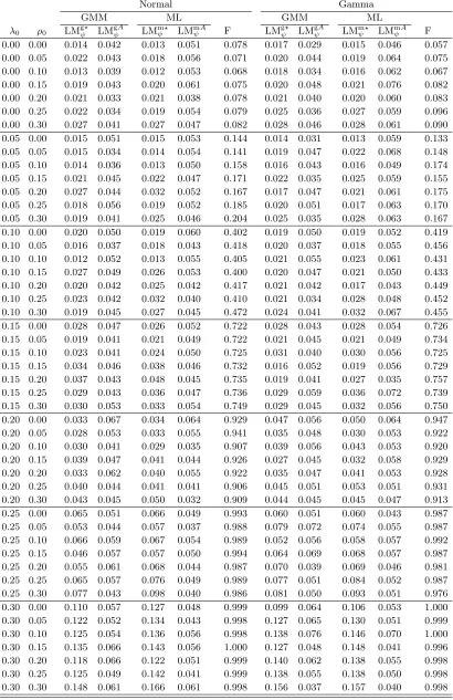
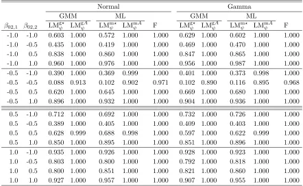
In the case of tests for the contextual effects in Table 2, we only use DGP 2 to study the size and power
316
properties of test statistics. For the size analysis, we set β02 = 02×1 and let λ0 and ρ0 vary between 0.1
to 0.6. For the power analysis, we set λ0 = 0.3 and ρ0 = 0.2, and let elements of β02 take on values from
318
{−1,−0.5,0.5,1}. All Monte Carlo simulations are based on 1000 repetitions.
Finally, we need to specify the set of moment functions for the GMM approach. As we mentioned before,
320
we are interested in the case where the number of instruments is kept fixed as the number of observations grows
without a bound. Therefore, we choose a simple set of moment functions: Q1r = Jr Xr, WrXr, Wr2Xr
,
322
U1r=JrWrJr−tr JrWrJr
Jr/tr Jr
andU2r=JrWr2Jr−tr JrWr2Jr
Jr/tr Jr
.
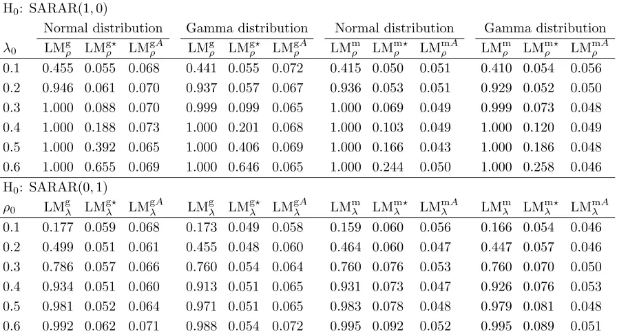
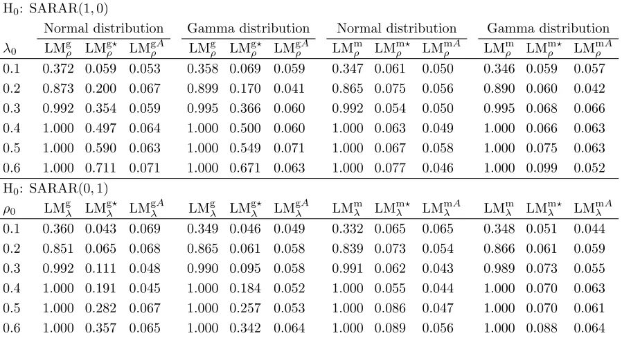
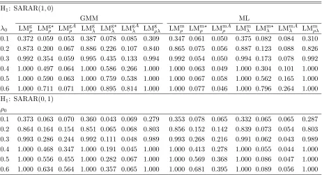
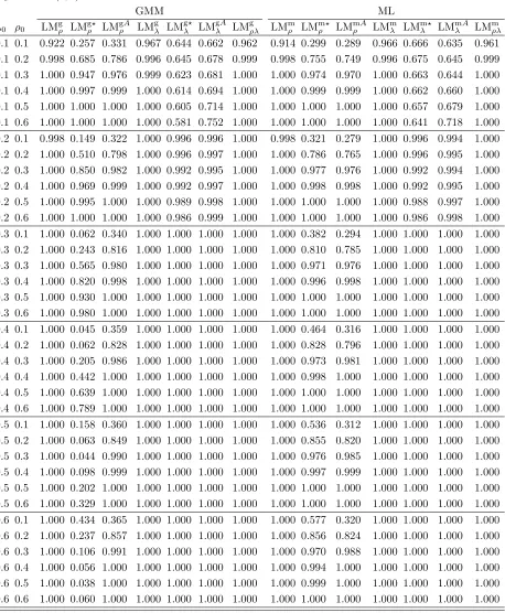
8. Results for Endogenous Effects and Correlated Effects
324
In this section, we investigate the finite sample properties of the test statistics for endogenous effects and correlated effects. In the following, we first evaluate the empirical rejection frequencies of each test under
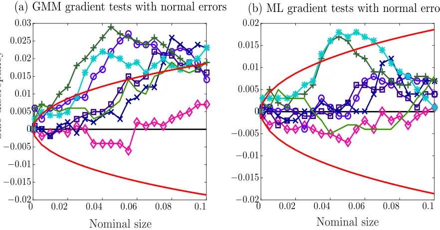
[image:17.612.73.539.371.508.2]the null hypothesis, and then provide a power analysis for each test.
8.1. Results on Size Properties
328
To present simulation results on size properties, we use the P value discrepancy plots suggested in Davidson
and MacKinnon (1998), which are based on the empirical distribution functions (edf) of p-values. Let τ be
a test statistic, and τj forj = 1, . . . ,Rbe theR realizations ofτ generated in a Monte Carlo experiment.
Let F(x) be the cumulative distribution function (cdf) of the asymptotic distribution of τ evaluated at x.
Then, the p-value associated with τj, denoted by p(τj), is given by p(τj) = 1−F(τj). An estimate of the
cdf of p(τ) can be constructed simply from the edf ofp(τj). Consider a sequence of points denoted byxi for
i= 1, . . . , mfrom the interval (0,1). Then an estimate of cdf ofp(τ) is given by
b F(xi) =
1 R
R
X
j=1
1 p(τj)≤xi
. (8.1)
As stated in Davidson and MacKinnon (1998), there is no decisive way to choose the sequencexifrom (0,1).
In practice, the main attention is typically paid to the Type-I errors which are set at levels smaller than or equal to 10%. We choose the following sequence and focus on levels smaller than or equal to 10%.
{xi}mi=1 ={0.001 : 0.001 : 0.010 0.015 : 0.005 : 0.990 0.991 : 0.001 : 0.999} (8.2)
The P value discrepancy plot is defined as the plot ofFb(xi)−xi againstxi under the assumption that
the true data generating process is characterized by the null hypothesis. If F(x) approximate to the finite
330
sample distributio