One way and two way cost allocation in hub network problems

Munich Personal RePEc Archive

One-way and two-way cost allocation in

hub network problems

Bergantiños, Gustavo and Vidal-Puga, Juan

15 May 2018

Online at

https://mpra.ub.uni-muenchen.de/97935/

One-way and two-way cost allocation in hub

network problems

G. Berganti˜nos †1 and J. Vidal-Puga ‡1

1_{Universidade de Vigo, 36310 Vigo, Spain}

May 15, 2018

Abstract

We consider a cost allocation problem arising from a hub network problem design. Finding an optimal hub network is NP-hard, so we start with a hub network that could be optimal or not. Our main objective is to divide the cost of such network among the nodes. We consider two cases. In the one-way flow case, we assume that the cost paid by a set of nodes depends only on the flow they send to other nodes (including nodes outside the set), but not on the flow they receive from nodes outside. In the two-way flow case, we assume that the cost paid by a set of nodes depends on the flow they send to other nodes (including nodes outside the set) and also on the flow they receive from nodes outside. In both cases, we study the core and the Shapley value of the corresponding cost game.

Keywords: game theory, hub network, cost allocation, core, Shap-ley value.

1

Introduction

Hub networks play a fundamental role in modelling telecommunication, transportation, and parcel delivery systems. Assume that there are users located at different geographical nodes who need to send a certain flow of data or goods to each other through costly connections. A planner needs to locate an optimal number of hub facilities at some nodes so that each non-hub node is connected to exactly one non-hub and all the non-hubs are connected

∗_{This work is partially supported by research grants ECO2014-52616-R from the}

Span-ish Ministerio de Econom´ıa y Competitividad, ECO2017-82241-R from the SpanSpan-ish Min-isterio de Econom´ıa, Industria y Competitividad, GRC 2015/014 from Xunta de Galicia, and 19320/PI/14 from Fundaci´on S´eneca de la Regi´on de Murcia.

†_{E-mail: [email protected]}

to one another at a reduced cost (due to economies of scale). Hence, the optimal flow of data/goods between any pair of origin-destination nodes has a length of at most four: It must go from the point of origin to its assigned hub (when the origin is not itself a hub), then to the hub assigned to the destination (if it is a different node) and finally to the destination (again, if it is not itself a hub). This topology is applied to Internet connections (Bailey, 1997), telecommunications between local networks (Greenfield, 2000), satel-lite communication (Helme and Magnanti, 1989), airline networks (Bryan and O’Kelly, 1999; Yang, 2009), small package delivery (Sim et al., 2009), and biofuel supply chains (Roni et al., 2017).

Several classes of hub problems have been studied. Recent examples include Contreras et al. (2017), Jankovic et al. (2017), Azizi (2018), Azizi et al. (2018), Alumur et al. (2018), and G¨uden (2018).

The main issue addressed in these papers is the study of algorithms for computing optimal ways of sending goods between the nodes in such a way that the total cost is minimized. Of course, location of the hubs plays a relevant role in the minimization problem. See Alumur and Kara (2008) and Farahani et al. (2013) for surveys on this literature.

Once we have computed the optimal (or quasi optimal) hub network, another issue is how to divide the cost associated with such hub network among the nodes. This question has been successfully addressed in sev-eral kinds of problems. We mention some of them. Guardiola et al. (2009) study production-inventory problems where players share production pro-cesses and warehouse facilities. Berganti˜nos et al. (2014), Berganti˜nos and Kar (2010), Bogomolnaia and Moulin (2010), Dutta and Mishra (2012), Trudeau (2012) and Trudeau and Vidal-Puga (2017) consider the cost of connecting agents to a source. Moulin (2014) considers users that need to connect a pair of target nodes in a network. Perea et al. (2009) consider the problem of sharing the profits associated with a supply chain problem. Alcalde-Unzu et al. (2015) consider the cost of cleaning a river.

trans-portation problem in a network. We associate a cooperative game, we study the core, and we propose an allocation in the core based on the Shapley value (Shapley, 1953). Besides, we provide an axiomatic characterization of such allocation.

However, few papers have studied the cost sharing issue associated with hub problems. We mention three of them.

Skorin-Kapov (1998) studies p-hub allocation problems, where p hubs must be optimally allocated. Several cooperative games are considered de-pending on who the agents are (nodes or pairs of nodes) and what coalitions can do (whether they must use the optimal network for the whole problem or can construct the optimal network of the reduced problem induced by the coalition). He studies the core of such games. Some games have an empty core but others have not. Finally, he considers the nucleolus of such games. Skorin-Kapov (2001) studies hub-like networks, which involve a p-hub median problem where direct connection between nodes is possible. More-over, there are savings when the traffic is high. He defines several associated cooperative games where the set of agents are the links. He shows that some of them can have an empty core, in other cases the core is a singleton, and in other cases it has many points.

Matsubayashi et al. (2005) consider the case where the number of hubs to be located is arbitrary, there is a cost of opening a hub, and there is a congestion cost associated with nodes (the greater the flow through a node, the greater its cost). They also define an associated cooperative game and study its core. In the cooperative game, players are the nodes and the characteristic function is defined assuming that each coalition cooperatively constructs a network. Moreover, each coalition assumes that the rest of the nodes do not establish any hub nodes and the coalition can determine the routing of all the traffic generated by the other nodes. Given this, they prove that the core could be empty, but they find a sufficient condition for the non-emptiness of the core and propose an allocation in the core when this sufficient condition is satisfied.

The three papers mentioned above follow a similar approach. The first step is to consider a class of hub problems, the next is to associate a coop-erative game with each problem in the class, and the last one is to study the core of such problems. If the core is nonempty, an allocation in the core could be considered as a nice way of sharing the cost among agents.

we assume that the cost paid by a set of nodesS depends on the flow they send to other nodes (including nodes outside S) and also on the flow they receive from nodes outsideS. For instance, if you are travelling and you use your mobile phone outside your country, the amount you pay depends on the calls you make and also on the calls you receive.1 On the other hand, you usually have to pay a minimum fare even in case you do not make calls, and only receive them. As far as we know this is the first paper considering this case.

Our main contributions are twofold. First, we study the existence of core allocations. Second, unlike Skorin-Kapov (1998, 2001) and Matsubayashi et al. (2005), we also characterize axiomatically rules that belong to the core and also satisfy other nice properties.

We now summarize our results for the one-way flow case. We consider two cooperative games associated with each hub problem and related to those presented by Skorin-Kapov (1998). In both games, the set of agents is the set of nodes. Nevertheless, the way in which we compute the cost game is different. In the first game, we consider that a network (which can be optimal or not) has been already constructed and nodes can use only the hubs associated with such network. Thus, we define the cost of a subset of nodesS as the cost of sending the flow of all agents inS using only the hubs available in the network. In the second game, we consider that each set of nodes can construct the hub network they want. Thus, we define the cost of a subset of nodesS as the cost of the optimal network we need for sending the flow of all agents inS.

We study the cores of both games. The core of the first game has many points. In any allocation in the core, each node pays the cost of sending its flow and the cost of any hub is divided in any way among the nodes that use such hub. As opposed, the core of the second game could be empty.

We study the Shapley value of the first game. In particular, we prove that the Shapley value corresponds to the allocation where each node pays the cost of sending its flow and the cost of any hub is divided equally among the nodes that use it. Thus, the Shapley value belongs to the core. We also provide two axiomatic characterizations of it. The first one uses core selec-tion and equal treatment on hubs. Core selecselec-tion says that the allocaselec-tion must be in the core. Suppose that the cost of a hub increases. Consider a pair of agents such that both use the hub. Equal treatment on hubs says that the allocation to both agents change in the same amount. Alternatively, consider a pair of agents such that no one use the hub. Equal treatment on hubs also says that their cost allocations change in the same amount. The

1

second characterization uses positivity (no node can obtain profits), equal treatment of hubs, independence of irrelevant hubs (nodes are not affected by a change in the cost of hubs that they do not use), and independence of irrelevant flows (if the flow between two nodes increases, then the other nodes should not be affected).

We now summarize our results for the two-way flow case. The study is similar to the one-way flow case. We associate two games with this setting. The first game is concave and hence its core is non empty. It consists of the convex hull of the vector of marginal contributions. As opposed, the second game may have an empty core.

We study the Shapley value of the first game. Since the game is concave, it belongs to the core. We prove that the Shapley value corresponds to the allocation where the cost of sending flow between any pair of nodes is divided equally between both nodes. Besides, the cost of each hub is divided equally between the nodes that use the hub. Finally, we provide two axiomatic characterizations. The first one uses core selection, equal treatment on hubs, and equal treatment on flows (if there is flow between a pair of nodes and it increases then both nodes must be affected in the same way). The second characterization uses positivity, independence of irrelevant hubs, independence of irrelevant flows, equal treatment on hubs, and equal treatment on flows.

The paper is organized as follows. In Section 2, we present the model. In Section 3, we study the one-way flow case, where the nodes are only interested in sending or receiving flow, but not both. In Section 4, we study the two-way flow case, where the nodes are interested in both sending and receiving flow. In Section 5 we give some examples. In Section 6, we present the conclusions.

2

The model

We consider situations where a group of agents, located at different locations, want to send and receive some specific good, which is sent through a costly network. Besides, we should locate some hubs at the agents’ locations. All hub agents are connected to each other and each non-hub agent is connected only to a hub agent. We now introduce the model formally.

N ={1, . . . , n} is a finite set of nodes (also called agents).

C = (cij)_i,j∈N is a cost matrix. For eachi, j∈N, cij is the cost of sending

a unit of flow from node ito node j. We assume cii= 0, cij =cji ≥0 and

cik≤cij+cjk for alli, j, k ∈N.

F = (fij)_i,j∈N is the flow matrix. For each i, j ∈N, fij represents the

amount of flow from nodei to node j. We assume fij ≥0 and fii = 0 for

all i, j ∈ N. Notice that we do not assume fij = fji, i.e. the flow is not

Each coordinate in d = (di)i∈N indicates the cost of maintaining or

constructing a hub at the respective node. We assumedi≥0 for alli∈N.

Scalar α ∈ [0,1] is the discounting factor of the cost when flow goes between a pair of hubs. Namely, if node i and node j are both hubs, then the cost of sending a unit of flow from node ito node j is αcij (instead of

cij).2

The first issue is to locate an optimal number of hubs, selected from the set of nodes. Besides, each non-hub is linked to exactly one hub and all the hubs are connected to each other. The triangle inequality cik ≤ cij +cjk

assures that the optimal path origin-destination uses at most two hubs. When there is a hub in node i ∈ N, we say with some abuse of notation that nodeiis a hub. Otherwise, we say that nodeiis a non-hub.

A hub network on N is determined by a nonempty set H ⊆ N and a function h : N \H −→ H such that h(i) is the hub linked to non-hub i. LetH be the set of all hub networks onN. For notational convenience, we writeh(i) =iwheni∈H, so thath is a function fromN onto H. Besides, we also write hfor the network associated with the functionh. Namely

h={{i, h(i)}:i∈N\H}.

Thus, given two nodesi, j ∈N, flow from node i to nodej goes first from nodei to hubh(i), then to hubh(j) and finally to node j (i=h(i) and/or h(i) =h(j) and/orh(j) =j are possible).

The cost of a hub network h is given by

X i∈N

X j∈N

c_ih(i)+αc_h(i)h(j)+c_h(j)j

fij+ X i∈H

di.

For simplicity, we denote

λh_ij = c_ih(i)+αc_h(i)h(j)+c_h(j)j

fij

so that the cost is

X i∈N

X j∈N

λh_ij +X

i∈H

di.

A hub networkh∈ H where

min

h∈H

  

X i∈N

X j∈N

λh_ij +X

i∈H

di   

is reached is called optimal. Since H is finite, there is always at least one optimal hub network.

2

A generalization would be to assume that these costs are given by another cost matrix

Ch_{= c}h ij

i,j∈N withc h

We define ahub network problem as a tupleP = (N, C, F, d, α, h), where h is a hub network.

Notice that we do not assume h to be an optimal hub network. We know that computing an optimal hub network is NP-hard. Thus, in many practical situations we use heuristics to decide the hub network h to be constructed. Hence, we do not know exactly if such hub network is optimal or not. We make a very weak assumption onh, all hubs are needed in order to send the flow. Namely, for all k ∈ H there exist i, j ∈ N with fij > 0

andk∈ {h(i), h(j)}. Ifhis an optimal hub network the assumption holds. In case h has been obtained using some heuristics, it seems reasonable to assume that the heuristics can detect when a hub is needed.

We now define c(P) as the cost associated with the hub network h. Namely,

c(P) =X

i∈N X j∈N

λh_ij +X

i∈H

di. (1)

In many cases after finding an optimal (or quasi optimal) hub network, we need to divide the cost of such network among the nodes. A rule is a function R that assigns to each hub network problem P an allocation R(P)∈RN satisfying

X i∈N

Ri(P) =c(P). (2)

Our aim is to study the cost allocation problem generated by each hub network problemP. We are interested in studying allocations both fair and stable. The idea is to propose desirable properties and try to find a rule satisfying many of them.

2.1 Properties

We consider two cases depending on the needs of the agents. In theone-way flow case, we assume that each agent is only interested in the outgoing flow (the case where each agent is only interested in the ingoing flow is analogous). In the two-way flow case, each agent is interested in both outgoing and ingoing flow.

We now define several properties. Since the definitions in the one-way and two-way are quite similar (some of them are exactly the same), we only define it once.

The first property says that no agent should obtain profit.

Positivity (P os) For any hub network problemP and eachi∈N, we have Ri(P)≥0.

we say that nodes i and j are equal when several conditions hold: First, fik = fjk for all k ∈ N \ {i, j} (in the two-way case we should add the

condition fki =fkj for allk ∈N \ {i, j}). Second, fij =fji. Third, i∈H

if and only if j ∈ H (namely, node i is a hub if and only if node j is a hub). Forth, {i, k} ∈ h if and only if {j, k} ∈ h (namely, if nodes i and j are nonhubs then both are connected to the same hub). Fifth, for each

{i, k},{j, k} ∈h,cik =cjk.

Equal Treatment of Equals (ET E) For any hub network problemPand each pair of equal nodesi, j∈N, we have that Ri(P) =Rj(P).

The next property says that if a node does not send any flow in the one-way flow case (respectively, a node does not send nor receive any flow in the two-way flow case), then it pays nothing.

Null Flow (N F) For any hub network problem P and each i ∈ N such that fij = 0 for all j ∈ N \ {i} (in the two-way we must add the

conditionfji = 0 for all j∈N \ {i}), we have thatRi(P) = 0.

The next property says that if the flow from node ito nodej increases, then in the one-way flow case nodeicannot pay less, whereas in the two-way flow case nodeicannot pay less and also node j cannot pay less,

Flow Monotonicity (F M) For any pair of hub network problems P = (N, C, F, d, α, h) andP′ = (N, C, F′, d, α, h) such that there existi, j∈

N satisfying fij ≥fij′ and fkl =f_kl′ otherwise, then Ri(P) ≥Ri(P′)

(in the two-way we must add the conditionRj(P)≥Rj(P′)).

The next property says that if the cost of a hub increases, then no node requiring such hub could pay less. Before giving the formal definition we introduce some notation.

For each S ⊆ N, let H_Sof ⊆ H denote the set of hubs used for sending the flow of agents inS. Namely,

H_Sof ={k∈H:∃i∈S, j ∈N withfij >0 andk∈ {h(i), h(j)}}.

Notice thatH_Sof ⊆His the set of hubs used by nodes inSin the one-way flow case.

Giveni∈N, we writeH_iof instead ofH_{of_i}. Notice thatH_Sof =S i∈SH

of i

for all S⊆N.

For each S⊆N, letH_Stf ⊆H denote the set of hubs used for sending or receiving the flow of agents inS. Namely,

Notice thatH_Stf ⊆His the set of hubs used by nodes inSin the two-way case.

Given i∈N, we write H_itf instead of H_{tf_i}. Again, H_Stf =S i∈SH

tf i for

allS ⊆N.

Hub Monotonicity (HM) For any pair of hub network problems P = (N, C, F, d, α, h) andP′ _{= (N, C, F, d}′_{, α, h) such that there existsk∈}

N satisfyingdk≥d′kanddj =d′j otherwise, then for each agentisuch

that k∈H_iof (in the two-way flow case, we replace H_iof by H_itf), we have thatRi(P)≥Ri(P′).

The next property says that if the cost of a link increases, then the two agents located at its vertices could not pay less. This property coincides for the one-way and two-way flow cases.

Cost Monotonicity (CM) For any pair of hub network problems P = (N, C, F, d, α, h) and P′ _{= (N, C}′_{, F, d, α, h) such that there exists}

i, j ∈ N satisfying cij ≥ cij′ and ckl = c′kl otherwise, then we have

thatRi(P)≥Ri(P′) and Rj(P)≥Rj(P′).

Assume that the cost of some hubdk decreases. It is then clear that ifh

was an optimal hub network in the original problem it will be also optimal in the new problem. How should agents be affected? The next two properties provide an answer to this question.

The first one says that agents that use hub k or do not use hub k are affected in the same way.

Equal Treatment on Hubs (ET H) For any pair of hub network prob-lemsP = (N, C, F, d, α, h) and P′ = (N, C, F, d′, α, h) such that there existsk ∈N satisfying dk ≥d′k and dj =d′j otherwise, then for each

pair of agentsi, j such that k∈H_iof ∩H_jof or k /∈H_iof ∪H_jof (in the two-way flow case, we replace k ∈H_iof ∩H_jof by k∈ H_itf ∩H_jtf and k /∈H_iof ∪H_jof by k /∈H_itf ∪H_jtf), we have that

Ri(P)−Ri P′=Rj(P)−Rj P′.

The second property says that agents that do not use hub k are not affected.

Independence of Irrelevant Hubs (IIH) For any pair of hub network problems P = (N, C, F, d, α, h) and P′ = (N, C, F, d′, α, h) such that there exists k ∈ N satisfying dk ≥ d′k and dj = d′j otherwise, then

Ri(P) = Ri(P′) for each agenti such that k /∈H_iof (in the two-way

We now introduce a similar property to IIH but with flows instead of hubs. Assume that node i increases its flow to some other node j. In the one-way flow case, all nodes but i should not be affected. In the two-way flow case, all nodes butiand j should not be affected.

Independence of Irrelevant Flows (IIF) For any pair of hub network problems P = (N, C, F, d, α, h) and P′ = (N, C, F′, d, α, h) such that there existj, k∈N satisfying 0< f_jk′ ≤fjk andf_j′′_k′ =fj′_k′ otherwise,

thenRi(P) =Ri(P′) for each agenti∈N\ {j} (in the two-way flow

case, we replacei∈N \ {j} by i∈N \ {j, k}).

The next property is not reasonable in the one-way flow case but it is in the two-way case. It says that a variation of flow affects the sender and the receiver in the same way.

Equal Treatment on Flows (ET F) For any pair of hub network prob-lemsP = (N, C, F, d, α, h) andP′ = (N, C, F′, d, α, h) such that there existk, l∈N satisfying 0< f_kl′ ≤fkl andfij′ =fij otherwise, we have

that

Ri(P)−Ri P′=Rj(P)−Rj P′

for all pair of agentsi, j such that{i, j}={k, l} or{i, j} ∩ {k, l}=∅.

2.2 Cooperative game concepts

We finally introduce some well-known concepts of cooperative game theory. Acost game is a pair (N,c) whereˆ N is the set of agents and ˆc: 2N _→R

is a cost function satisfying ˆc(∅) = 0. Each nonempty subset S ⊆ N is called a coalition, and ˆc(S) denotes the cost of providing the needs of all agents inS. Since ˆcdepends onN, we write ˆc instead of (N,ˆc).

We say that ˆc is concave if for all l ∈ T ⊂ S ⊆ N, we have ˆc(S)−

ˆ

c(S\ {l})≤c(T)ˆ −ˆc(T\ {l}).

We now introduce two well-known solution concepts in cooperative game theory: the core (Gillies, 1959) and the Shapley value (Shapley, 1953).

The core of a cost game ˆcis defined as

Core(ˆc) =

(

y∈RN :X

i∈N

yi = ˆc(N) and X i∈S

yi ≤ˆc(S)∀S ⊂N )

.

The Shapley value is defined as the allocation Sh(ˆc) such that

Shi(ˆc) = X S⊂N\{i}

|S|! (n− |S| −1)!

n! [ˆc(S∪ {i})−ˆc(S)]

for each i∈N.

The main motivation behind the Shapley value is “fairnes”. Namely, to provide a fair way of dividing the total cost among the agents. Shapley (1953) proved that the Shapley value is the unique allocation satisfying the following four properties: efficiency (the total cost is divided among the agents), symmetry (symmetric agents must pay the same), null agent (if an agent does not increase the cost of any coalition, such agent should pay nothing) and additivity (the allocation should be additive on the cost function). Later on, several authors provided other characterizations of the Shapley value which made it very popular as a fair outcome. It is well-known that the Shapley value can be outside the core even when the core is non-empty. Nevertheless, when the cost game is concave, the Shapley value belongs to the core.

3

One-way flow

In this section we assume that nodes are interested only in the outgoing flow. Namely, the cost of a group of nodes depends only on the outgoing flow of such nodes. We first associate to each hub network problem a cost game. Later, we study its core and its Shapley value.

For each hub network problemP, we associate the cost gamecof_P where for each S ⊆N,cof_P (S) is the cost of sending the flow of all nodes in S to all nodes through the hub networkh. The cost game cof_P models situations where the hub networkh (with associated set of hubsH) has already been constructed. Thus,dcould be considered as a vector of maintenance costs. This cost game is formally defined as

cof_P (S) =X

i∈S X j∈N

λh_ij + X

i∈H_Sof

di (3)

for allS⊆N. When no confusion arises we writecof(S) instead ofcof_P (S).

Remark 3.1 Skorin-Kapov (1998) associates several games with each hub network problem. One of them, denoted as c1, is closely related to cof. In

our model, when h has a fixed number of hubs and di = 0 for all i, cof

coincides with c1. Thus, cof can be considered as a generalization of c1 to

our model. Besides, Skorin-Kapov (1998) proves that the core ofc1 contains

3.1 The core

In the next theorem we prove that the core ofcof _{is the set of cost allocations}

in which each agent pays the cost of sending its flow. Besides, the cost of any hub is divided in any way among the agents that use the hub for sending their flow.

Theorem 3.1 For each hub network problemP, the core ofcof _{is nonempty,}

and it is given by

Corecof=

(

x∈RN :P

i∈Nxi =c(P), xi =Pj∈Nλhij +yi∀i∈N

where y∈RN+ and

P

i∈Syi ≤ P

i∈H_Sofdi∀S ⊂N )

.

Proof. “⊇” is obvious. We now prove “⊆”. Let x ∈Core cof

. For each i ∈ N, we define yi = xi −Pj∈Nλhij. Then, for each i ∈ N, xi can be

rewritten asxi =Pj∈Nλhij +yi. Since,x∈Core cof

, for each S⊂N,

cof(S) =X

i∈S X j∈N

λh_ij+ X

i∈H_Sof

di≥ X i∈S

xi = X i∈S

X j∈N

λh_ij+X

i∈S

yi

and thus P

i∈Syi ≤ P_i∈Hof S

di. It only remains to prove that y ∈ RN+.

Suppose not. Let j∈N be such thatyj <0. Thus, X

i∈N\{j}

xi = X i∈N

xi−xj =cof(N)−xj

=X

i∈N X k∈N

λh_ik+X

i∈H

di− X k∈N

λh_jk −yj

= X

i∈N\{j}

X k∈N

λh_ik+X

i∈H

di−yj

> X

i∈N\{j}

X k∈N

λh_ik+X

i∈H

di

sinceH_Nof_\{j} ⊆H,

≥ X i∈N\{j}

X k∈N

λh_ik+ X

i∈H_Nof_\{j}

di=cof(N \ {j})

which is a contradiction.

Skorin-Kapov (1998) also considers another game, denoted as c∗₁, which is obtained as c1 but assuming that each coalition can build their optimal

Nevertheless, we can study an intermediate situation. Assume that the optimal hub network is not unique. Thus, we should decide which one to construct. It could be the case that some agents prefer one over another. Thus, we can define the cost of a coalition as the minimum over all optimal hub networks. Namely, for eachS ⊆N,

c∗(S) = min

h∈H,his optimal

n

cof_P(h)(S)o

whereP(h) is the hub network problem induced by the optimal hub network h.

Next example shows that the core of c∗ can be empty.

Example 3.1 Let N ={1,2,3}, cij = 1for all i, j∈N, f12=f23=f31=

1, f21 = f32 = f13 = 10, α = 1, and di = 6 for all i ∈ N. There exist

three optimal hub networks

hi _i∈N, corresponding to putting a single hub in each node i ∈ N, respectively. We will see that each two-node coalition would prefer a different hub location. We start with coalition {1,2}. We computecof_P(h1

)({1,2}), c

of P(h2

)({1,2}), and c

of P(h3

)({1,2}):

cof_P(h1₎({1,2}) =

X i∈{1,2}

X j∈N

λh_ij1 + X

i∈H_{of1,2_}

di

=λh₁₂1 +λh₁₃1 +λh₂₁1 +λh₂₃1+d1

= (c12)f12+ (c13)f13+ (c21)f21+ (c21+c13)f23+d1

= (1)1 + (1)10 + (1)10 + (1 + 1)1 + 6 = 29.

cof_P(h2₎({1,2}) =

X i∈{1,2}

X j∈N

λh_ij2 + X

i∈H_{of1,2_}

di

=λh₁₂2 +λh₁₃2 +λh₂₁2 +λh₂₃2+d2

= (c12)f12+ (c12+c23)f13+ (c21)f21+ (c23)f23+d2

= (1)1 + (1 + 1)10 + (1)10 + (1)1 + 6 = 38.

cof_P(h3₎({1,2}) =

X i∈{1,2}

X j∈N

λh_ij3+ X

i∈H_{of1,2_}

di

=λh₁₂3 +λh₁₃3+λh₂₁3+λh₂₃3+d3

= (c13+c32)f12+ (c13)f13+ (c23+c31)f21+ (c22)f23+d3

Thus, coalition {1,2} would prefer the hub to be at1, because

cof_P(h1

)({1,2}) = 29<min

n

cof_P(h2

)({1,2}), c

of P(h3

)({1,2})

o

.

Analogously, coalition {1,3} would prefer to locate the hub at 3, because

cof_P(h3₎({1,3}) = 29<min

n

cof_P(h1₎({1,3}), c

of

P(h2₎({1,3})

o

;

and coalition{2,3} would prefer to locate the hub at 2, because

cof_P(h2₎({2,3}) = 29<min

n

cof_P(h1₎({2,3}), c

of

P(h3₎({2,3})

o

.

Let x be a core allocation. Then

100 = 2c∗(N) = 2 (x1+x2+x3)

= (x1+x2) + (x1+x3) + (x2+x3)

≤cof_P(h1

)({1,2}) +c

of P(h3

)({1,3}) +c

of P(h2

)({2,3})

= 29 + 29 + 29 = 87,

which is a contradiction.

Thus, the core of c∗ is empty.

3.2 The Shapley value

We now study the Shapley value ofcof, which we call theShapley rule. We first give an explicit formula. Later, we provide two axiomatic characteriza-tions.

In next theorem we prove that in the Shapley rule each node pays the cost of sending its flow. Besides, the cost of any hub is divided equally among the nodes that use the hub for sending their flow.

Theorem 3.2 For each hub network problem P and each i∈N,

Shi

cof_P = X

j∈N

λh_ij+ X

j∈H_iof

dj

n

k∈N :j∈H_kofo

.

Proof. We consider several cost games. Let c0 be defined as c0(S) =

P i∈S

P

j∈Nλhij for each S ⊆ N. For each j ∈ N, let cj be defined as

cj(S) = dj if j ∈ HSof and cj(S) = 0 otherwise. Thus, for each S ⊆ N,

cof_{(S) = c}0_{(S) +}P

j∈Ncj(S). Since the Shapley value is additive on c,

we have that for each i ∈N, Shi cof

=Shi c0

+P

j∈NShi cj

. Since c0 is an additive game (there exists a ∈ RN such that for each S ⊆ N, c0(S) =P

j∈Sai) we deduce thatShi c0

=P

the cost gamecj_{, all agents that use hubj(i.e. allk∈N such thatj ∈H}of k )

are symmetric and the agents that do not use hub j are dummy. Thus, for each j∈N,

Shi cj

=

  

dj

n

k∈N:j∈H_kofo

ifj∈H_iof 0 otherwise,

from where it is straightforward to check the result.

We now introduce a new property of rules which says that we must select an allocation in the core of the problem.

Core Selection (CS) For any hub network problem P, we have that

R(P)∈Corecof_P .

There are some relations between CS and some ot the properties intro-duced in Subsection 2.1.

Proposition 3.1 (a) CS implies P os. (b) P os, IIH and IIF imply CS.

Proof. (a) Assumex∈Core cof

. Then, for all i∈N,

xi=cof(N)− X j∈N\{i}

xj ≥cof(N)−cof(N\ {i})≥ X j∈N\{i}

λh_ij ≥0.

(b) LetRbe a rule satisfyingP os,IIH, andIIF. FixS ⊂N. Letε >0 and definePS,ε _{= N, C, F}S,ε_{, d}S_{, α, h}

as the problem obtained from P by turning all positive flows not used byS intoεand all hub costs not used by S into zero. Formally,

f_ijS,ε =

ε ifi /∈S and fij >0

fij otherwise

and

dS_k =

0 ifk /∈H_Sof dk otherwise.

Then,cof_PS,ε(N)≤

P i∈S

P

j∈Nλhij + P

k∈HSofdk+a(P)εwhere

a(P) =|{fij :fij >0}|max (

λh_ij fij

:fij >0 )

Now,

X i∈S

Ri(P)IIH=+IIF X i∈S

Ri PS,ε=cof_PS,ε(N)−

X i∈N\S

Ri PS,ε

P os

≤ cof_PS,ε(N)≤

X i∈S

X j∈N

λh_ij + X

k∈HSof

dk+a(P)ε

=cof_P (S) +a(P)ε

which impliesP

i∈SRi(P)≤cofP (S) because a(P) does not depend onε.

CS does not imply neitherIIH norIIF. The rule in which each node pays the cost of sending its flow and the cost of each hub is paid equally by the nodes that use the most expensive hubs among those that use that hub satisfies CS but not IIH. The rule in which each node pays the cost of sending its flow and the cost of each hub is paid equally by the nodes sending more flow through this hub satisfiesCS but notIIF.

In next proposition we prove that the Shapley rule satisfies all the prop-erties introduced in Subsection 2.1 for the one-way flow case.

Proposition 3.2 The Shapley rule satisfies P os, ET E, CS, N F, F M, HM, CM, ET H, IIH and IIF.

Proof. From Theorem 3.2, we deduce that Sh cof

satisfies P os, F M, HM, andCM. Ifiandjare equal inP, then it is not difficult to check that iand j are symmetric incof_{. Now, symmetry of the Shapley value implies}

that Sh cof

satisfies ET E. Anyi∈N with fij = 0 for all j ∈N \ {i} is

a dummy player in cof. Hence, its Shapley value is zero, and so Sh cof

satisfiesN F. LetP, P′ andkbe given as in the definition ofET H andIIH. Giveni, j∈N such thatk∈H_iof ∩H_jof, under Theorem 3.2,

Shi

cof_P −Shi

cof_P′

= dk−d

′ k n

l∈N :k∈H_lofo

=Shj

cof_P −Shj

cof_P′

.

Giveni, j∈N such thatk /∈H_iof ∪H_jof, by Theorem 3.2

Shi

cof_P −Shi

cof_P′

= 0 =Shj

cof_P −Shj

cof_P′

.

HenceSh cof

satisfiesET H. Giveni∈N such thatk /∈H_iof, from Theo-rem 3.2 we know thatShi cof

does not depend ondk, and soShi

cof_P =

Shi

cof_P′

and hence Sh cof

satisfies IIH. Let P, P′ and i, j, k be given as in the definition of IIF. From Theorem 3.2 we have that Shi cof does

not depend onfjk. Hence, Sh cof

satisfiesIIF. From Proposition 3.1, it satisfiesCS.

Theorem 3.3 (a) The Shapley rule is the unique rule satisfying CS and ET H.

(b) The Shapley rule is the unique rule satisfying P os, IIH, IIF, and ET H.

Proof. (a) By Proposition 3.2 the Shapley rule satisfies these properties. We now prove the uniqueness. Let R be a rule satisfying CS and ET H. Let P = (N, C, F, d, α, h) be any hub network problem. For each K ⊆H, letPK = N, C, F, dK, α, h

withdK defined as follows:

dK_i =

0 ifi∈H\K di otherwise.

For all k ∈ N, let Nk,0 = ni∈N :k /∈H_iofo, Nk,1 = ni∈N :k∈H_iofo, nk,0 =

Nk,0

and nk,1 = Nk,1

for allk ∈N. ET H implies that, for each

k∈K, there existxk,0 _{and x}k,1 _{such that for alli∈N}k,0_,

Ri PK−Ri

PK\{k}=xk,0 (4)

and for alli∈Nk,1

Ri PK

−Ri

PK\{k}=xk,1. (5)

SinceN =Nk,0∪Nk,1 and

X i∈N

Ri PK− X i∈N

Ri

PK\{k}=dk,

we have that for allk∈K,

nk,0xk,0+nk,1xk,1=dk. (6)

The equivalence relation inN defined as

i∼j⇔ ∃k∈K :i, j∈Nk,1 ori, j∈Nk,0

determines a partition PK of N. It is straightforward to check that the cost game cof_PK(N) =

P S∈PKc

of

PK(S). So CSimplies that

P

i∈SRi PK

= cof_PK(S) for all S ∈ PK. Moreover, any PL with L ⊂ K is a refinement of

PK, so P

i∈SRi PL

=cof_PL(S) for all S∈ PK.

We now consider several cases.

Case 1. Assume that PK has at least two components. Given k ∈ K, there exist S, S′ ∈ PK such that k ∈ S ∩ H and S′ ⊆ Nk,0. Besides, cof_PK\{k}(S′) =c

of

PK(S′). Thus,

cof_PK S

′

=X

i∈S′

Ri PK

(4)

= X

i∈S′

Ri

PK\{k}+ S′

xk,0

CS

= cof

PK\{k} S

′

+ S′

xk,0=cof PK S

′

+ S′

which implies that xk,0 _{= 0. Under (6), x}k,1 ₌ dk

nk,1 for all k ∈ K. Under

(5), for each i∈N,

Ri PK=Ri

PK\{k}+ dk nk,1.

Repeating the same reasoning, we deduce that for eachi∈N,

Ri PK

=Ri

P∅+ X

k∈H_iof

dk

nk,1.

Since R satisfies CS, under Theorem 3.1, Ri P∅ = P_j∈Nλh_ij +yi for all

i∈N, where 0≤yi ≤P_j∈Hof i d

∅

j. By definition of d∅, we have d∅j = 0 for

allj ∈H. Since H_iof ⊆H, we deduceyi = 0 and so

Ri

P∅=X

j∈N

λh_ij.

By Theorem 3.2,

Ri PK= X j∈N

λh_ij + X

k∈Hiof

dk

nk,1 =Shi P

K

.

Case 2. Assume nowPK={N}. We consider several subcases.

Case 2.1. AssumeK ={k}. SinceR satisfies CS, under Theorem 3.1,

X i∈Nk,0

Ri

P{k}= X

i∈Nk,0

X j∈N

λh_ij+ X

j∈Nk,0

yi

wherey∈RN+ and

0≤ X i∈Nk,0

yi ≤ X

j∈Hof

N k,0

d{_jk}= 0

which impliesP

i∈Nk,0y_i= 0. Thus,

X i∈Nk,0

Ri

P{k}= X

i∈Nk,0

X j∈N

λh_ij.

On the other hand,

X i∈Nk,0

Ri

P{k}(4)= X

i∈Nk,0

Ri

P∅+nk,0xk,0= X

i∈Nk,0

X j∈N

λh_ij +nk,0xk,0

which impliesxk,0 _{= 0. So, for eachi∈N}k,0_,

Ri

P{k}= X

j∈N

λh_ij =Shi

Under (6),xk,1 ₌ dk

nk,1. So, for each i∈Nk,1,

Ri

P{k}=Ri

P∅+ dk nk,1 =

X j∈N

λh_ij + dk

nk,1 =Shi

P{k}.

Case 2.2. Assume now|K|>1. We proceed by induction on|K|. Hence, we assumeRPK′=ShPK′when |K′|<|K|. We have three cases:

Case 2.2.1. Assume first nk,0 = 0 for some k ∈ K. Under (5), for all i∈N =Nk,1_,

Ri PK

=Ri

PK\{k}+xk,1.

Hence,

X i∈N

Ri PK= X i∈N

Ri

PK\{k}+nxk,1

and thus

xk,1=

P

i∈NRi PK

−P

i∈NRi PK\{k}

n =

dk

nk,1.

Now for alli∈N =Nk,1,

Ri PK

=Ri

PK\{k}+ dk nk,1.

By induction hypothesis, for alli∈N

Ri PK

= X

j∈N

λh_ij+ X

j∈H_iof

dK_j \{k} nk,1 +

dk

nk,1

= X

j∈N

λh_ij+ X

j∈H_iof

dK_j

nk,1 =Shi P

K

.

Case 2.2.2. Assume now nk,1 _{= 0 for some k ∈K. By (4), R}

i PK =

Ri PK\{k}+xk,0 for alli∈N =Nk,0. The rest of reasoning is analogous

to the previous case and we omit it.

Case 2.2.3. Finally, assumenk,0_{>0 andn}k,1_{>0 for all k∈K. We can}

assume w.l.o.g. 1,2 ∈ K. Let i1 ∈N1,1 and i2 ∈N1,0. Since PK = {N}, we know that there exists some k ∈ K such that either i1, i2 ∈ Nk,1 or i1_{, i}2 _∈Nk,0_{. Assume w.l.o.g. that either i}1_{, i}2 _{∈ N}2,1 _{or i}1_{, i}2 _∈N2,0_{. For}

each k∈ {1,2} and each l ∈ {1,2}, letfl_{(k) ∈ {0,1} be defined such that}

il _∈Nk,fl_(k)

. Hence, we know thatf1_{(1) = 1 (becausei}1 _∈N1,1_),f2_{(1) = 0}

By induction hypothesis, for any k∈ {1,2}and any l∈ {1,2},

R_il PK

(4)(5)

= R_il

PK\{k}+xk,fl(k)=Sh_il

PK\{k}+xk,fl(k)

=X

j∈N

λh_il j+

X

j∈Hof

il

dK_j \{k} nj,1 +x

k,fl_(k)

.

Thus, for each l∈ {1,2},

x1,fl(1)−x2,fl(2) = X

j∈Hof

il

dK_j \{1}−dK_j \{2} nj,1 =

d1

n1,1f

l₍₁₎₋ d2

n2,1f

l_(2).

In particular, takinga=f1_{(2) =f}2_{(2) andl= 1,}

x1,1−x2,a= d1 n1,1 −

d2

n2,1a (7)

and takingl= 2,

x1,0−x2,a =− d2

n2,1a. (8)

Equations (6) for k = 1,2 and equations (7)-(8) can be written as a matrix equation as follows:

   

n1,1 _{0 n}1,0 ₀

0 n2,1 0 n2,0 1 −a 0 a−1 0 −a 1 a−1

    ·    

x1,1

x2,1 x1,0 x2,0

    =     d1 d2 d1

n1,1 − d 2

n2,1a

− d2

n2,1a

   

.

The determinant of the left matrix is an−n2,1

n 6= 0. Hence, the matrix equation has a unique solution given byxk,1= dk

nk,1 and xk,0= 0 for

allk∈ {1,2}. Thus,

Ri1 PK

(5)

= Ri1

PK\{1}+x1,1=Ri1

PK\{1}+ d1 n1,1

R_i2 PK

(4)

= R_i2

PK\{1}+x1,0=R_i2

By induction hypothesis,

R_i1 PK

=Sh_i1

PK\{1}+ d1 n1,1

T h.3.2

= X

j∈N

λh_i1_j+

X

k∈Hof

i1

dK_k\{1} nk,1 +

d1

n1,1

=X

j∈N

λh_i1

j+ X

k∈Hof

i1

dK_k nk,1

T h.3.2

= Sh_i1 PK

R_i2 PK

=Sh_i2

PK\{1}T h.=3.2 X

j∈N

λh_i2

j + X

k∈Hof

i2

dK_k\{1} nk,1

=X

j∈N

λh_i2_j+

X

k∈Hof

i2

dK k

nk,1

T h.3.2

= Sh_i2 PK

.

Since i1_{, i}2 _{were taken arbitrarily from N}1,1 _{and N}1,0_{, respectively, and}

these two sets form a partition ofN, we conclude thatRi PK=Shi PK

for all i∈N.

(b) It follows from part (a) and Proposition 3.1.

Remark 3.2 We now prove that the properties used in Theorem 3.3 are independent.

• Let R0 be defined as R0(P) = x+Sh cof

for some x ∈ RN with

P

i∈Nxi = 0 and xi 6= 0 for some i∈N. R0 satisfies IIH, IIF and

ET H, but fails CS and P os.

• Let ω ∈ RN be such that ωi >0 for all i∈ N and ωi 6= ωj for some

i6=j. Let R1 be defined for each P and eachi∈N as follows: R1_i (P) =X

j∈N

λh_ij+ X

j∈H_iof

ωi P

k∈N:j∈H_kofωk

dj.

R1 _{satisfies CS, P os, IIH, and IIF, but failsET H.}

• Let R2 _{be defined for each P and i∈N as follows:}

R2_i (P) =X

j∈N

λh_ij+X

j∈H

dj

n.

R2 satisfies P os, IIF and ET H, but fails CS and IIH.

• Let R3 be defined for each P and i∈N as follows:

R3_i (P) =

P k∈N

P

j∈Nλhkj

n +

X

j∈H_iof

dj

n

k∈N :j∈H_kofo

.

4

Two-way flow

In this section, we assume that nodes are interested in both outgoing and ingoing flow. Namely, the cost of a group of nodes depends on the outgoing and the ingoing flow of such nodes. We first associate to each hub network problem a cost game. Then, we study the core and the Shapley value of such game.

For each hub network problem P, we associate the cost game ctf_P where for each S ⊆N, ctf_P (S) is the cost of sending and receiving the flow of all nodes in S to and from all nodes through h. The cost game ctf_P models situations where an (optimal) hub network h (with associated set of hubs H) has already been constructed. Thus,dcan be considered as a vector of maintenance costs. We formally define this cost game as follows:

ctf_P(S) = X

(i,j)∈/(N\S)×(N\S)

λh_ij + X

i∈H_Stf

di (9)

for all S⊆N. When no confusion arises we write ctf _{instead ofc}tf P.

4.1 The core

In next theorem we prove that in the core allocations ofctf the cost of send-ing or receivsend-ing flow between two nodes is divided between them. Besides, the cost of any hub is divided among the nodes that use the hub for sending or receiving their flow. Before stating the theorem we need some notation.

Let Π ={π:N −→N :π biyective} be the set of orderings of agents in N. Given i∈N and j ∈H, Πij ⊂Π is the set of orderings such that node

iis the first that uses hub j, i.e. π(l) =iimplies j /∈H_πtf_(l′₎ for all l′ < l.

Theorem 4.1 For each hub network problem,ctf is concave. Moreover, the core is nonempty and given by the convex hull of the following set of vectors:

    

  

X j∈N:π−1

(j)>π−1

(i)

λh_ij+λh_ji+ X

j∈H_itf:π∈Πij

dj   

i∈N     

π∈Π

.

Proof. We first prove that N, ctf

is concave. Let l∈T ⊂S ⊆N. Since for each S′⊂N,H_Stf′ =

S

i∈S′H_itf, we have that

Then,

ctf(S′)−ctf S′\ {l}

= X

(i,j)∈/(N\S′_)×(N\S′₎

λh_ij+ X

i∈HS′

di

− X

(i,j)∈/(N\(S′_{\{l}))×(N\(S}′_\{l}))

λh_ij− X i∈H_Stf_′\{l}

di

= X

i∈N\S′

λh_il+ X

j∈N\S′

λh_lj+ X

i∈H_Stf′\H tf S\{l}

di.

Since all terms are non-negative,N \S ⊂N \T and (10), we have that

ctf(S)−ctf(S\ {l})≤ctf(T)−ctf(T \ {l}) which proves that N, ctf

is concave.

It is well-known that, when the cost game is concave, the core coin-cides with the Weber set. Thus, the core is the convex hull of the vectors of marginal contributions. Notice that the coordinate i of the vector of marginal contributions for π∈Π is

X j∈N:π−1_(j)>π−1_(i)

λh_ij +λh_ji+ X

j∈H_itf:π∈Πij

dj,

from where the result trivially holds.

Analogously to the one-way flow case, we consider an intermediate sit-uation between a fixed hub network and a variable hub network. Assume that the optimal hub network is not unique. We can define the cost of a coalition as the minimum over all optimal hub networks. Namely, for each S⊆N,

c∗∗(S) = min

h∈H,his optimal

n

ctf_P(h)(S)o

whereP(h) is the hub network problem induced by the optimal hub network h. Next example shows that the core of c∗∗ can be empty.

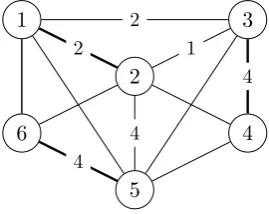
Example 4.1 Let P be such that N = {1,2, . . . ,6}, α = 1, f12 = f34 =

f56= 1, fij = 0 otherwise,d1 =d2=d3 = 1 anddi ≥4 otherwise. The cost

matrix is given in the following table:

cij 2 3 4 5 6

1 2 2 3 3 3 2 1 3 4 3

3 4 3 3

4 3 3

This hub problem is depicted in Figure 1.

1

2

3

4

5 6

2 1

2

4

4 4

Figure 1: cij = 3 when no specified. Flow goes from 1 to 2, from 3 to 4, and

from 5 to 6.

There exist three optimal hub networks h1_{, h}2_{, andh}3_{, corresponding to}

putting a single hub at either 1, 2 or 3, respectively. The cost of these net-works is 14 each. Hence, c∗∗(N) = 14. Moreover, nodes 1,2,3,4 can cover their own flow at cost7when the hub is located at2. Then,c∗∗({1,2,3,4}) = 7. Analogously, nodes 1,2,5,6 can cover their own flow at cost 9 when the hub is located at 1, so that c∗∗({1,2,5,6}) = 9. Analogously, nodes 3,4,5,6 can cover their own flow at cost 11 when the hub is located at 3, so that c∗∗({3,4,5,6}) = 11. Hence, a core allocation y should satisfy y1+y2+y3+y4 ≤7, y1+y2+y5+y6 ≤9, andy3+y4+y5+y6 ≤11. By

adding these inequalities and dividing by2, we deduce that P

i∈Nyi≤13.5.

Sincec∗∗(N) = 14, we deduce that the core ofc∗∗ is empty.

4.2 The Shapley value

We now study the Shapley value ofctf, which we also call theShapley rule. In next theorem, we prove that in the Shapley rule the cost of sending flow between a pair of nodes (λh

ij) is divided equally between both nodes. Besides,

the cost of any hub is divided equally among the nodes that use the hub for sending or receiving their flow.

Theorem 4.2 For each hub network problem P and each i∈N,

Shi

ctf=X

j∈N

λh ij+λhji

2 +

X

j∈Hitf

dj

n

k∈N :j∈H_ktfo

. (11)

Proof. It is well known that the Shapley value is the average of the vectors of marginal contributions. Thus,

Shi

ctf= 1

|Π|   

X π∈Π

X j∈N:π−1_(j)>π−1_(i)

λh_ij+λh_ji+ X

j∈H_itf X π∈Πij

Let Πij =

π∈Π :π−1(j)> π−1(i) . Clearly, |Πij|= |Π₂|. Hence, 1

|Π| X π∈Π

X j∈N:π−1

(j)>π−1

(i)

λh_ij +λh_ji= 1

|Π| X j∈N

X π∈Πij

λh_ij+λh_ji

= 1

|Π| X j∈N

|Πij|λh_ij +λh_ji

=X

j∈N

λh_ij+λh_ji 2

which is the first part of (11).

Let T = nk∈N :j∈H_ktfo and t = |T|. We still need to prove that

1

|Π|

P j∈Hitf

P

π∈Πijdj = P_j∈Htf i

dj

t . Clearly, it is enough to prove that

|Πij|

|Π| = 1t for allj∈H tf

i . Notice that Πij is the set of orderings in which the

predecessors ofiare not in T. In particular, Πij =Ss=1,...,n−t+1Πsij where

Πs

ij ={π ∈Πij :π(s) =i}. Hence, |Πij_|Π|| =Pn_s=1−t+1|

Πs ij|

|Π| . Moreover,

|Πs ij|

|Π| is

the probability of randomly picking up an order in Π satisfying that nodei is in positionsand it is preceded bys−1 nodes inN\T. Let|N\T|=n−t. Then, Π s ij |Π| =

n−t n ·

n−t−1 n−1 · · · · ·

n−t−s+ 2 n−s+ 2 ·

1 n−s+ 1 =

(n−s)!(n−t)! n!(n−t−s+ 1)! So

|Πij| |Π| =

(n−t)! n!

n−t+1

X s=1

(n−s)! (n−s−t+ 1)!

= (n−t)!t! n!

n−t+1

X s=1

(n−s)!

(n−s−t+ 1)!(t−1)! · 1 t

= 1_n

t

n−t+1

X s=1

n−s t−1

1 t.

Then, it is enough to prove that n_t

=Pn_s=1−t+1 n_t−−₁s

. This is trivially true whenn= 1. By induction hypothesis onn, and using Stidel formula:

n t =

n−1 t−1

+

n−1 t

=

n−1 t−1

+

n−t X s=1

n−1−s t−1

=

n−1 t−1

+

n−t+1

X s=2

n−s t−1

=

n−t+1

X s=1

n−s t−1

.

Core Selection (CS) For any hub network problem P, we have that

R(P)∈Corectf_P.

The analogous results for Proposition 3.1 also hold in the two-way flow case.

Proposition 4.1 (a) CS implies P os. (b) P os, IIH and IIF imply CS.

Proof. It is analogous to the proof of Proposition 3.1 and we omit it. CS does not imply neitherIIH norIIF. The rule in which each node pays half the cost of sending and receiving her flow and the cost of each hub is paid equally by the nodes that use the most expensive hubs among those that use that hub satisfies CS but not IIH. The rule in which each node pays half the cost of sending and receiving her flow and the cost of each hub is paid equally by the nodes sending more flow through this hub satisfies CS but notIIF.

In next proposition we prove that the Shapley rule satisfies all the prop-erties we have defined in Subsection 2.1 for the two-way flow case.

Proposition 4.2 The Shapley rule satisfies P os, ET E, CS, N F, F M, HM, CM, ET H, IIH, IIF andET F.

Proof. The proof for P os, ET E, CS, N F, F M, HM, CM, ET H, IIH andIIF is analogous to that of Proposition 3.2 (using Theorem 4.2 instead of Theorem 3.2 and Proposition 4.1 instead of Proposition 3.1) and we omit it.

LetP, P′ be given as in the definition of ET F. We consider two cases:

1. {i, j}={k, l}. Letλh′ theλh associated withP′. By Theorem 4.2,

Shi

ctf_P−Shi

ctf_P′

= λ

h ij−λh

′

ij

2 =Shj

ctf_P−Shj

ctf_P′

,

and henceSh ctf

satisfies ET F.

2. {i, j} ∩ {k, l}=∅. Under Theorem 4.2,

Shi

ctf_P−Shi

ctf_P′

= 0 =Shj

ctf_P−Shj

ctf_P′

.

Theorem 4.3 (a) The Shapley rule is the unique rule satisfyingCS,ET H and ET F.

(b)The Shapley rule is the unique rule satisfyingP os,IIH,IIF,ET H, and ET F.

Proof. (a) By Proposition 4.2 the Shapley rule satisfies these properties. We now prove the uniqueness. Let R be a rule satisfying CS, ET H and ET F.

LetP = (N, C, F, d, α, h) be a hub network problem. We assume di= 0

for all i∈H; the extension to positive hub costs is analogous to the proof of Theorem 3.3 and we omit it.

Let E = {(i, j) :fij >0} and, for each i ∈ N and e ∈ E, let ai(e) =

1 when node i is adjacent to e, and ai(e) = 0 otherwise. Denote E =

{e1, . . . , eγ}. We assume, w.l.o.g., e1 = (1,2). We also assume, w.l.o.g.,

e2 = (2,1) in case (2,1)∈E.

For eachε >0, letPε= (N, C, Fε, d, α, h) defined byf_ijε =εfor all (i, j) withfij >0, andfijε =fij = 0 otherwise.

Leta(P) de defined as in the proof of Proposition 3.1. Suppose that, for ε small enough, there exists xP ∈ RN with −7|E|a(P)ε≤ xP_i ≤ 7|E|a(P)ε for all i∈N such that

Ri(P) = X e∈E

λh_e 2 a

i_{(e) +x}P

i for all i∈N. (12)

Since Ri(P) does not depend onε, we deduce that for alli∈N

Ri(P) = X e∈E

λh_e 2 a

i_{(e) =}X j∈N

λh_ij+λh_ji

2 =Shi(P).

Hence, we just need to prove that (12) holds.

For each ek ∈ E, we define P−k = N, C, F−k, d, α, h with fe−kk = ε

andf_ij−k=fij otherwise. For notational convenience, we writeλh_k,fij−k and

ai(k) instead of λh_ek,f−ek

ij and ai(ek), respectively.

We proceed by induction on|E|. CaseE =∅ is not possible because H is nonempty and for each k∈ H we assume that there exist i, j ∈ N with fij >0 and k∈ {h(i), h(j)}.

Assume thenE ={e1}. In this case, P−1 =Pε. LetxPi = 0 ifi /∈ {1,2}

and xP_i =Ri(P)−λ

h

1

2 ifi∈ {1,2}. We prove that for all i∈N,xPi lies on

the interval [−7a(P)ε,7a(P)ε].

Let i /∈ {1,2}. By CS, Ri(P) ≤ ctf_P({i}) = 0. Since ai(e1) = 0 and

λh_e = 0 when e6=e1, (12) holds trivially.

Hence,

y1,1 = R1(P) +R2(P)−R1(P

−1_)−R 2(P−1)

2 .

By CS, 0 ≤ R1(P) +R2(P) = λh1 and 0 ≤ R1(P−1) +R2(P−1) ≤a(P)ε.

Hence,

y1,1∈

λh₁

2 −a(P)ε, λh₁

2 +a(P)ε

.

By induction hypothesis, xP−1

1 ∈[−a(P)ε, a(P)ε]. Thus,

R1(P) =R1 P−1

+y1,1 =x₁P−1 +y1,1 ∈

λh₁

2 −2a(P)ε, λh₁

2 + 2a(P)ε

.

and so (12) holds withxP

1 =R1(P)−λ h

1

2 .

Assume now (12) holds when|E|< γ and suppose|E|=γ. We consider several cases:

Case 1. γ = 2 and e2 = (2,1), so that E ={e1, e2}. Then, we proceed

as above definingy1,1 in the same way.

Case 2. Either γ >2 or e26= (2,1). Notice that this impliesn >2. Fix

i∈N. We consider two cases.

Case 2.1. ai(e) = 0 for all e∈E. We take xP_i = 0. Then, byCS, (12) holds becauseRi(P) = 0.

Case 2.2. There existsk∈E such that ai_{(k) = 1. Fix alsoe}

l∈E\ {ek}

with different adjacent nodes than ek. We can find such el because either

γ >2 or e2 6= (2,1).

ET F implies that there exist yk,0_{, y}k,1_{, y}l,0 _{and y}l,1 _{such that R}

j(P)−

Rj P−k=yk,a

j_(k)

and Rj(P)−Rj P−l=yl,a

j_(l)

for all j∈N.Since

X j∈N

Rj(P)− X j∈N

Rj

P−k=λh_k−λ h k

fk

ε,

we have

2yk,1+ (n−2)yk,0=λh_k+zk,1 (13)

wherezk,1=−λhk

fkε∈[−a(P)ε,0]. Analogously,

2yl,1+ (n−2)yl,0 =λh_l +zl,1 (14)

withzl,1∈[−a(P)ε,0].

On the other hand, Ri(P) =Ri(P−k) +yk,1 =Ri(P−l) +yl,a

i_(l)

. Hence,

yk,1−yl,ai(l)=Ri(P−l)−Ri(P−k)

by induction hypothesis,

= λ

h k

2 − λh_l

2 a

i_{(l) +x}P−l

i −xP

−k

withxP−l

i , xP

−k

i ∈[−7γ−1a(P)ε,7γ−1a(P)ε].

We define zk,0 =x_iP−l−xP_i−k ∈[−2·7γ−1a(P)ε,2·7γ−1a(P)ε] so that

yk,1−yl,ai(l)= λ

h k

2 − λh_l

2 a

i_{(l) +z}k,0_{. (15)}

We repeat the reasoning for some j ∈N adjacent to el (i.e. aj(l) = 1)

but not toek (i.e. aj(k) = 0). We can find such j because el has different

adjacent nodes thanek. Then, we get

yl,1−yk,0 = λ

h l

2 +z

l,0 ₍₁₆₎

withzl,0∈[−2·7γ−1a(P)ε,2·7γ−1a(P)ε].

Equations (13)-(14)-(15)-(16) form a system of linear equations given by

   

2 0 n−2 0 0 2 0 n−2 1 −ai_{(l) 0 a}i_(l)−1

0 1 −1 0

    ·    

yk,1 yl,1 yk,0

yl,0

    =      λh k+zk,1

λh_l +zl,1

λh k 2 −

λh l

2 ai(l) +zk,0

λh k 2 +zl,0

     .

The determinant of the first matrix is (n+ 2ai(l)−4)n. We consider several cases.

Case 2.2.1. ai(l) = 1. Then, (n+ 2ai(l)−4)n6= 0. Thus, the previous system of linear equations have a unique solution which is given foryk,1 by

yk,1 = λ

h k

2 + z (n−2)n

wherez= (n−2)zk,1_−nzl,1_{+ (n}2_{−4n+ 4)z}k,0_{+ (n}2_{−4n+ 4)z}l,0_.

Sincezk,1, zl,1, zk,0, zl,0∈[−2·7γ−1a(P)ε,2·7γ−1a(P)ε], we deduce that z∈[−2(2n2−6n+ 6)·7γ−1a(P)ε,2(2n2−6n+ 6)·7γ−1a(P)ε].

For n >2, we have 2(2n

2

−6n+6)

(n−2)n ≤6 and hence

z

(n−2)n ∈[−6·7

γ−1_a(P)ε,6·7γ−1_{a(P)ε]. (17)}

By induction hypothesis,

Ri(P) =Ri(P−k) +yk,1= X e∈E

λh e

2 a

i_{(e) +x}P−l

i +

z (n−2)n.

Case 2.2.2. ai_{(l) = 0 andn6= 4. Then, (n+ 2a}i_{(l)−4)n6= 0. Thus, the}

previous system of linear equations have a unique solution which is given foryl,0 by

yl,0 = z (n−4)n

wherez=−2zk,1+ (n−2)zl,1+ 4zk,0+ (−2n+ 4)zl,0.

Sincezk,1, zl,1, zk,0, zl,0∈[−2·7γ−1a(P)ε,2·7γ−1a(P)ε], we deduce that z∈

−3n·7γ−1a(P)ε,3n·7γ−1a(P)ε

.

For n≥3,n6= 4 we have _(n−6n_4)n ≤6 and hence

yl,0 ∈[−6·7γ−1a(P)ε,6·7γ−1a(P)ε]. (18) By induction hypothesis,

Ri(P) =Ri(P−l) +yl,0 = X e∈E

λh_e 2 a

i_{(e) +x}P−l

i +yl,0.

Let us definexP i =xP

−l

i +yl,0. By (18) andxP

−l

i ∈[−7γ−1a(P)ε,7γ−1a(P)ε],

we deduce thatxP_i ∈[−7γa(P)ε,7γa(P)ε].

Case 2.2.3. ai(l) = 0 and n= 4. Then, (n+ 2ai(l)−4)n = 0. In this case we replace equation (16) by eitheryk,0_−yl,0_=zlk,0 _oryl,1_−yk,1 ₌ λhl

2 −

λh k

2 +zlk,1, withzlk,·∈[−2·7γ−1ε,2·7γ−1ε]. Now the resulting determinant

is non zero. The rest of the proof is similar and we omit further details. (b) It follows from (a), Proposition 4.2, and Proposition 4.1.

Remark 4.1 We now prove that the properties used in Theorem 4.3 are independent.

• Let R0 be defined as R0(P) = x +Sh ctf

for some x ∈ RN with

P

i∈Nxi = 0 and xi 6= 0 for some i ∈ N. R0 satisfies IIH, IIF,

ET H and ET F, but failsCS and P os.

• Let ω ∈ RN be such that ωi >0 for all i∈ N and ωi 6= ωj for some

i6=j. Let R1 be defined for each P and eachi∈N as follows:

R1_i (P) =X

j∈N

λh_ij+λh_ji 2 +

X

j∈H_itf

ωi P

k∈N:j∈H_ktfωk

dj.

R1 _{satisfies CS, P os, IIH, IIF and ET F, but fails ET H.}

• Let R2 be defined for each P and i∈N as follows:

R2_i(P) =X

j∈N

λh ij+λhji

2 +

X j∈H

dj

n.

• Let R3 _{be defined for each P and i∈N as follows:}

R3_i (P) =

P k∈N

P j∈N

λh_kj

n +

X

j∈H_itf

dj

n

k∈N :j∈H_ktfo

.

R3 satisfies P os, ET H, IIH and ET F, but failsCS and IIF.

• Let R4 be defined for each P and i∈N as follows:

R4_i(P) =X

j∈N

λh_ij+ X

j∈H_itf

dj

n

k∈N :j∈H_ktfo

.

R4 _{satisfies CS, P os, IIH, IIF and ET H but fails ET F.}

5

Some examples

We now present some examples where we compute the Shapley rule and compare it with the rule considered in Matsubayashi et al., 2005.

We first provide an example of a hub problem in which the proportional rule proposed by (Matsubayashi et al., 2005, Theorem 3.1) does not belong to the core, whereas the one-way Shapley value does.

Example 5.1 Let P be such that N = {1,2,3}, α = 0.1, di = 3 for all

i∈N, c12= 1, c13=c23= 10,f13=f23= 1 andfij = 10otherwise. There

is no congestion cost. In this problem, there exists a unique optimal hub network. It has three hubs, one at each node, and the total cost is 33. The proportional rule gives the cost allocationu∗ = (8.643,8.643,15.714), which does not belong to the core because cof_{({1,2}) = 13 <2·8.643 = u}∗

1+u∗2.

As opposed, the Shapley rule gives the cost allocation (5,5,23), which does belong to the core.

We now apply our results to Example 4.3 in Matsubayashi et al. (2005).

Example 5.2 (Example 4.3 in Matsubayashi et al. (2005)) LetP be such that N = {1,2, . . . ,7}, α = 0.2, di = 65 for all i ∈N. The flow and

cost matrices are both symmetric and given in the following respective ta-bles3:

fij 2 3 4 5 6 7

1 0.1 0.1 1.5 1.5 1 1 2 0.1 1.5 1.5 1 1 3 1.5 1.5 1 1

4 0.1 1 1

5 1 1

6 f67

3

cij 2 3 4 5 6 7 7

1 1.5 1.5 59 58 96 93 87 2 1.5 60 59 96 93 86 3 60 59 97 94 87

4 2 106 110 116

5 107 111 117

6 4 10

The cost matrix assigns two columns to node7. The first one applies when node 7 represents Osaka. The second one applies when node 7 represents Seoul. The other nodes represent London (node1), Brussels (node2), Paris (node3), Washington (node4), Ottawa (node5), and Tokyo (node6). There is also a congestion factor that increases the cost at each node by 0.1% of the flow that goes through it.

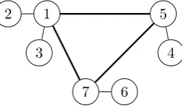
When f67 = 0.1 or f67 = 1, and node 7 represents Osaka, the optimal

hub network is depicted in Figure 2, with hubs at nodes 1, 5 and 7.

1 2

3 4

5

6 7

Figure 2: Optimal hub network which arises in Example 4.3(a) and Example 4.3(b) in Matsubayashi et al. (2005).

When f67 = 25 and node 7 represents Osaka, or f67 = 10 and node 7

represents Seoul, the optimal hub network is depicted in Figure 3, with hubs at nodes 1, 5, 6 and7.

1 2

3 4

5

6 7

Figure 3: Optimal hub network which arises in Example 4.3(c) and Example 4.3(d) in Matsubayashi et al. (2005).

We now compare the rule suggested by (Matsubayashi et al., 2005, Theo-rem 3.2), also denoted asu∗, and the one-way Shapley rule.4 The allocation

4

for Osaka is represented in next table (in parenthesis, the value of f67 for

each column):

Osaka (f67= 0.1) Osaka (f67= 1) Osaka (f67= 25)

i u∗_i Shi u∗i Shi u∗i Shi

1 109.6 107.5 109.4 107.5 102.0 113.4 2 109.6 115.2 109.4 115.2 102.0 121.1 3 109.6 115.2 109.4 115.2 102.0 121.1 4 144.7 146.6 144.5 146.6 135.6 151.2 5 144.7 133.6 144.5 133.6 135.6 138.1 6 143.6 153.8 147.8 157.4 199.9 166.0 7 143.6 133.7 147.8 137.4 199.7 165.8

For each i ∈ N, let fi· = P_jfij denote the flow that leaves node i. Next

table shows the cost allocation per unit of flow (yi/fi·):

Osaka (f67= 0.1) Osaka (f67= 1) Osaka (f67= 25)

i u∗_i/fi· Shi/fi· u∗i/fi· Shi/fi· u∗i/fi· Shi/fi·

1 21.08 20.67 21.05 20.67 19.61 21.81 2 21.08 22.15 21.05 22.15 19.61 23.29 3 21.08 22.15 21.05 22.15 19.61 23.29 4 21.92 22.22 21.89 22.22 20.55 22.91 5 21.92 20.24 21.89 20.24 20.55 20.92 6 28.16 30.15 24.63 26.24 6.662 5.534 7 28.16 26.22 24.63 22.90 6.656 5.527

The main differences between the one-way Shapley rule and u∗ are the following:

1. Under the Shapley rule, it is preferable to be a hub because hub nodes pay less than the other nodes connected to it. Under u∗, nodes con-nected to the same hub pay the same. For instance, when f67 = 1,

node1is a hub and nodes2 and3 are connected to node1. Under the Shapley rule, node1 pays less than nodes 2 and 3. Under u∗, node 1 pays the same as nodes2 and 3.

2. When f67 increases from 0.1 to 1 and the other flows do not change,

the optimal hub network does not change. Under the Shapley rule, the cost increase is charged to the nodes responsible for it (nodes 6 and 7), leaving the rest unaffected. Under, u∗, nodes 6 and 7 pay more whereas the rest of nodes pay less.

3. Whenf67increases from1to25and the other flows do not change, the