Productive Performance and Technology Gaps using a Bayesian Metafrontier Production Function: A cross country comparison

Munich Personal RePEc Archive

Productive Performance and Technology

Gaps using a Bayesian Metafrontier

Production Function: A cross-country

comparison.

Economou, Polychronis and Malefaki, Sonia and Kounetas,

Konstantinos

Department of Civil Engineering, University of Patras, Greece,

Department of Mechanical Engineering and Aeronautics, University

of Patras, Greece, Department of Economics, University of Patras,

Greece

13 June 2019

Online at

https://mpra.ub.uni-muenchen.de/94462/

Productive Performance and Technology Gaps

using a Bayesian Metafrontier Production

Function: A cross-country comparison

Economou Polychronis

, Malefaki Sonia

, and Kounetas Konstantinos

1

Department of Civil Engineering, University of Patras, Greece

Department of Mechanical Engineering and Aeronautics,

University of Patras, Greece

3

Department of Economics, University of Patras, Greece

Abstract

Growth theory argues on the role of heterogeneity that can lead to multiple regimes examining countries performance. A meta-production stochastic function under a Bayesian perspective has been developed to estimate technical efficiencies across countries over a time period. The metafrontier model is used to highlight heterogeneity among cluster of countries revealing catch up phenomena. The es-timation procedure relies on the solution of an optimization problem and on the concept of the upper orthant order of two multivariate normal random variables. The proposed models are applied in a real dataset consisting of 109 countries for a 20-year period from 1995-2014. The productive performance differential and the associated technology gaps were investigated using two distinct frontiers (OECD vs non-OECD countries). Empirical results reveal that heterogeneity indeed plays a significant and distinctive role in determining technological gaps.

keywords:Technological heterogeneity,Bayesian approach, Metafrontier, Spillovers,

JEL Classifications: C11,C23,C51,D24,O10,

1

Introduction and motivation

One of these problems refers to the fact that several entities under different techno-logical structures (i.e countries, industries, firms, regions) can face dissimilar produc-tion possibilities that differ over time. These producproduc-tion possibilities can be attributed firstly to the different way the specific entities transform the available set of inputs to the set of outputs and secondly, to differences due to the environment that they oper-ate. The first one is attributed to the technological status that each entity uses while the second considers that each entity is conditional to the technological group that belongs. These conditions may inhibit entities to choose the best available technology and is closely related with two concepts; technological hierarchy and heterogeneity. The first term, hierarchy, conceptually refers to a specific regulatory framework while the second one has a more arbitrary meaning (Dosi et al., 2010). Thus, an attractive av-enue for further empirical research is to assume that each production entity belongs to each own technological group. However, such this technological isolation (Tsekouras et al., 2016, 2017) can not be meaningfully pursued using classical approaches. Recog-nition of this significant limitation has motivated many researchers to use/borrow the differential geometry term of envelope and to develop the concept of meta-production function.

The initiation by the development of a theoretically meta-production function (Hayami, 1969; Hayami and Ruttan, 1970) and the refinement and transposition of this concept to a stochastic frontier (SFA) and a data envelopment analysis (DEA) framework (Battese and Rao, 2002; Battese et al., 2004; ODonnell et al., 2008) concluded in the metafron-tier production function1_{. The major drawback of Battese et al. (2004) approach is that}

in the second step of their method the metafrontier production function is calculated using linear programming methods (Huang et al., 2014) and thus does not allow for the existence of statistical properties (Amsler et al., 2017; Huang et al., 2014).

Motivated by this limitation, we propose a Bayesian metaproduction function us-ing an SFA approach to estimate technology gaps. To the best of our knowledge, there is no other attempt for calculating technology gaps while the incorporation of a SFA approach is more suitable for panel data (Tsionas, 2002) but still rare in applied re-search (Tsionas, 2002; Griffin and Steel, 2007; Tabak and Tecles, 2010). In addition, the Bayesian SFA provides a more realistic approach (Chen et al., 2015) and leads to more accurate efficiency estimations (Tsionas, 2002; Tabak and Tecles, 2010)) and incorporate model uncertainty (Tabak and Tecles, 2010) and caters for heterogeneity (Tsionas, 2002)

Heterogeneity in the Bayesian context (Van den Broeck et al., 1994) has been stud-ied through the use of hierarchical models (Tsionas, 2002; Huang et al., 2014) and in the inefficiency factor using covariates in the distribution of the non-negative error component (Koop et al., 1997). In advance, (Griffin and Steel, 2004, 2007) provide models of observed heterogeneity using flexible and non-parametric mixtures of inef-ficiency while Gal´an et al. (2015) discuss unobserved inefinef-ficiency heterogeneity with the inclusion of a random parameter in the inefficiency distribution. On the other hand, heterogeneity stemming from differentials in the characteristics of the production en-vironment has never been explored in the literature in a Bayesian perspective.

1_{In the first stage efficiency estimates are provided for each group while in the second stage the}

In this study we exploit a dataset consisting of 109 countries for a 20-year pe-riod from 1995-2014 and investigate the productive performance differential and the associated technology gaps using a metafrontier Bayesian approach from two distinct frontiers. The first one consists of countries that belong to OECD while the second one to countries that do not belong at OECD. The incorporation of a metaproduction function under a Bayesian perspective permits us to give statistical properties to the first stage estimates for the meta-efficiency scores. Furthermore, allows the incorpo-ration, into the model, of any available, theoretical or based on previous studies, prior information through the prior distributions of the parameters. This prior information is combined with the information contained in the observed data to provide new insights into the nature of the data. This is very important in similar datasets since information maybe is available from previous economic studies. Finally, it is worth mentioning that since a simulated sample from the posterior distribution is always available, even for the unobserved variables, it is straight forward to estimate any quantity of interest.

Our empirical results reveal that heterogeneity indeed plays multi-edged roles in the spillover effects through different channels. Among them, we can distinguish technol-ogy choice set, absorptive capacity and capabilities, human capital level and localized technical change. Moreover, the existence of significant technology gaps especially for the non-OECD countries groups reveal the serious obstacles regarding technology spillovers Bardhan and Lapan (1973) and support the idea of non catch-up phenom-ena. Most importantly, the different trends that each group follows underline a world of divergence during the 20-year period of examination.

The rest of the paper is organized as follows. In Section 2 the stochastic frontier model and the formulation of the metafrontier production function is presented. In Section 3 the frontier model under a Bayesian framework is given in a coherent way by presenting in detail all the necessary steps to apply the MCMC algorithm. In Section 4 the proposed Bayesian metafrontier production model is presented. In the following section the proposed analysis is applied to a data set obtained by the World Bank by using two distinct frontiers (OECD vs non-OECD countries). Finally. some concluding remarks are given in the last section.

2

Stochastic frontier model and formulation of

metafron-tier production function

Stochastic frontier production functions have been used, extensively, in a large number of empirical studies to account the possible existence of technical inefficiencies in pro-duction. Stemming from the seminal paper of Aigner et al. (1977) and Meeusen and van den Broeck (1977) and following Kumbhakar and Lovell (1998), it is as-sumed that the production technologySmodels the transformation of a vector of inputs

x′_it(j)= (x_1it(j),x_2it(j), ...,x_kit(j))∈Rk

+that each unitiin the groupj(for example coun-tryiin geographical region or organization j) can employ at timetto produce a vector of outputy′_it(j) = (y_1it(j),y_2it(j), ...,y_pit(j))∈R₊p, The technology setSprovides a de-scription of all technologically feasible relationships between inputsxand outputsy

Note, that all units (hereafter countries) do not make necessarily the most of the inputsx′_it(j)given the technology embodied in the production function and may produce less than it might due to a degree of inefficiency. One should recognize that this degrees of inefficiency might be effected by the geographical region or the organizationjthat a country belongs since none country is technologically isolated (Tsekouras et al., 2016, 2017). On the other hand, random shocks, that are assumed to be independent by any technical inefficiency, can increase or decrease the final production of a specific country. These characteristics cause extra heterogeneity in the final production and for that reason a flexible model should be defined to describe the production of thei−th country in the j−thgroup (out of totalJgroups) at yeart(over the time period ofT years). As a consequence, the stochastic production function can be expressed as:

Y_it(j)=f(x_it(j),β(j))exp(vit(j)−uit(j)), t=1, . . . ,T, i=1, . . . ,nj,j=1, . . . ,J. (1) (see for example Aigner et al. (1977); Battese and Rao (2002), wherex_it(j)is the vec-tor of the values of some functions of the inputs used by thei−thunit in thet−th time period for the j−thgroup,β(j) the(k+1)×1 parameter vector,vit(j)a normal error term andu_it(j)>0 a measure of technical inefficiency. Usually, the unobservable random errors are independently distributed withv_it(j)∼N(0,σ2

v)anduit(j) is a non negative random variable for each group. The above model is usually referred as Error Component Model (ECM) (Battese and Coelli) due to the fact that the final production of every country is a result of two errors components.

By taking natural logarithm in both sides of equation (1) we have

lnY_it(j)=lnf(x_it(j);β_(j)) +v_it(j)−u_it(j), t=1, . . . ,T, i=1, . . . ,nj,j=1, . . . ,J. (2) A frequently used mathematical representation for f(x_it(j);β_(j))is

f(x_it(j);β_(j)) =exp

x′_it(j)β_(j). (3) Based on the relation (1) and choosing the above function form for f(x_it(j);β(j)), Bat-tesse and Coelli (1992) achieved to expressed a country’s technical efficiency, belong-ing to a specific group, by the followbelong-ing expression:

T E_it(j)= Yit(j)

exp(x′_it(j)β(j)+vit(j))

≡e−uit(j) ₍₄₎

each country could produce, comparing not only with the group that belongs, but also with all the other countries, if it had the opportunity to use all the available technology Amsler et al. (2017). Thus, the metafrontier function model is expressed by

Y_itM≡f(x_it(j);βM), (5) whereβM _{denotes the vector of parameters for the metaproduction function satisfying} the conditionx′_it(j)βM≥x′_it(j)β(j)for all j=1, . . . ,JBattese et al. (2004).

The introduction of metafrontier analysis (Amsler et al., 2017) as an approach that allows the investigation of the interrelationships between different technologies Battese et al. (2004) can be used in order to explain differences in production opportunities that can be attributed to available resource endowments, economic infrastructure and other characteristics of the physical, social and economic environment in which production takes place ODonnell et al. (2008); Kontolaimou et al. (2012). Moreover, it accounts for structure of national markets, national regulations and policies, cultural profiles and legal and institutional frameworks Halkos and Tzeremes (2011), different ownership types Casu et al. (2013) and different rate of access and acceptance of General Purpose Technologies-GPT (Kounetas et al., 2009).

All these features allow us to estimate the so-called Technology Gap Ratio (TGR), that measures the ratio of the output for the frontier production function for thei−th country in the j−thgroup at timetrelative to the potential output, given the observed input, that is determined by the metafrontier production function given by

T GR(x_it(j)) = f(xit(j);β(j))

f(x_it(j);βM₎ = e−uM_it

e−uit(j) (6)

Related to that, ODonnell et al. (2008) extended the Battese et al. (2004) framework for the technical efficiency with respect to the group’s frontier, to the estimation of the technical efficiency with respect to the metafrontier production function, defined as T EMFit=T Eit(j)∗T GR(xit(j)).

3

Frontier models – A Bayesian approach

Some previous efforts in the direction of Bayesian modeling the frontier model can be found in Van den Broeck et al. (1994), Griffin and Steel (2004) and Griffin and Steel (2007). In the present section we present in a coherent way the Bayesian approach for parameter estimation by describing in details every single step for applying the Bayesian analysis. Initially the likelihood function is derived and prior distributions are assigned to the parameter of the model. Due to the complex structure of the posterior distribution direct inference is not possible on it, thus a MCMC algorithm is proposed for sampling from it.

3.1

Likelihood function

as

Y_it∗=x′_itβ+vit−uit (7) From equation (7) and assuming thatvit∼N(0,σv2)anduit∼Exp(λu), it holds that

Y_it∗|θ,u∼N(x′_itβ−uit,σv2)

whereθ= (β,λu,σv2)are the parameters of the model. As a consequence, the likeli-hood conditionally onuit’s is given by

L(Y∗|θ,u)∝

n

∏

i=1

T

∏

t=1

1

σv exp

− 1

2σ2

v

y∗_it−x′_itβ+uit

2

∝ 1

σnT v

exp n

∑

i=1

T

∑

t=1

− 1

2σ2

v

y∗_it−x′_itβ+uit

2 !

.

3.2

Assign priors to the parameters - The full posterior

distribu-tion

A conjugate prior is assigned to the regression parametersβ β∼Nk+1(βprior,Σβ)

wherek+1 is the dimension ofβ(including the constant term). The point estimate

βprior - possibly obtained from previous or draft analysis - reflects the researcher’s belief on the most likely region of the parameter space. The choice ofΣ_{β reflects} his/her degree of confidence in this point estimate. A reasonable choice forΣ_{β, under} the assumption of no multicollinearity, for a moderate degree of confidence on the point estimate could beΣ_{β =10}4_{Ik+1, whereIk+1is the identity matrix of size}k+1.

For the inverse of the variance ofvit,σ−2

v , and the parameterλufor the exponential distribution ofuitconjugate priors are assigned. More specifically,

σ_v−2∼Gamma(αv,γv)

λu∼Gamma(αu,γu).

with meansαv/γv,αu/γuand variancesαv/γv2,αu/γu2 respectively that reflect avail-able information from previous studies. Otherwise, non informative priors such as Gamma(2,1/2)orGamma(2,1)are used forσ−2

Thus, the full posterior distribution for the regression model is given by

π(θ,u|data) =L(Y∗|θ,u)π(u|θ)π(θ) =L(Y∗|θ,u)π(u|λu)π(λu)π(σ

2

v)π(β)

= 1 σnT v exp n

∑

∑

2σ2

v

y∗_it−x′_itβ+uit

2 !

·

λαu−1

u exp(−γuλu)·

1

σ2

v

αv−1

exp −γv 1 σ2 v · exp −1

2(β−βprior)

′_Σ−1

β (β−βprior) · n

∏

∏

λuexp(−λuuit)I(uit>0)

which can be expressed as

π(θ,u|data) =

1

σ2

v

nT₂ +αv−1

exp − 1 σ2

v

γv+ 1 2 n

∑

∑

y∗_it−x′_itβ+uit

2 !! · exp −1

2(β−βprior)

′_Σ−1

β (β−βprior)

·

λnT+αu−1

u exp −λu γu+ n

∑

∑

∏

∏

I(uit>0).

3.3

The MCMC algorithm

Due to the complicated structure of the posterior distribution, direct inference is in-feasible. Thus, MCMC methods are adopted. From the full posterior distribution it is obvious that a data augmentation procedure for the unobserveduit should be followed as an initial step in each iteration of the MCMC algorithm. The MCMC algorithm can be described by the following steps:

Step 1. For eachiandtsample from the full conditional posterior distribution ofuit uit|β,λu,σv,data∼N+

−yit+x

′

itβ−λuσv2,σv2

using the current values ofβ,λu,σv

Step 2. For eachℓ∈0,1, . . . ,ksample from the full conditional posterior distribution of

βℓ

βℓ|β(−ℓ),σv,λu,u,data∼N

µ_βℓ,σ_β2

ℓ

where

µ_βℓ= σ2

vµℓ+σℓ2 n

∑

∑

x_it(ℓ)yit+uui−x

′

it(−ℓ)β(−ℓ)

σ_v2+σ_ℓ2

n

∑

∑

x2_it(ℓ)

σ2

βℓ=

σ2

vσℓ2

σ2

v+σℓ2 n

∑

∑

x2_it(ℓ)

andβ_(−ℓ)is the coefficient vector ofβwithoutβℓ,σℓ2is theℓth diagonal element ofΣ2_,µ

ℓis theℓth element of the mean vector ofβpriorandxit(ℓ) is the theℓth element ofxit

Step 3. Sample from the full conditional posterior distribution ofσ2

v

σ_v2|β,λu,u,data∼InvGamma nT

2 +αv−2,γv+ 1 2 n

∑

∑

yit−x

′

itβ+uit

2 !

Step 4. Sample from the full conditional posterior distribution ofλu

λu|β,σv,u,data∼Gamma nT+αu,γu+ n

∑

∑

4

Estimating the parameters of the metafrontier

pro-duction function

In the classical, deterministic approach the metafrontier model is determined by choos-ing a specific function (of the same of form of each frontier) such that the predicted value for the metafrontier is larger than or equal to the predicted value from the stochas-tic frontier for all entities and groups.The best metafrontier is identified by minimizing the sum of absolute deviations or the sum of squares of the deviations . The first cri-terion assigns the same weight to all the observations in the sample while the latter assigns larger weights to the deviations associated with observations that have larger technology gap ratios. Both these approaches are similar and for that reason the identi-fication of metafrontier model is only presented under the minimization of the sum of squares of deviations.

4.1

Minimum Sum of Squares of Deviations

the optimization problem:

min S=min T

∑

∑

x′_itβM−x′_itβˆ(j)

2

s.t. x′_itβM≥x′_itβˆ(j) (8)

wherex′_itβˆ(j)is defined with correctly associateβˆ(j)withx

′

itfor the jth cluster. In the Bayesian framework βˆ_(j) are not given as point estimates but can be de-scribed by their posterior distribution obtained by the procedure dede-scribed in the pre-vious section. As a result a similar procedure can not be adopted without any further modification. Sinceβˆ(j)are given as random variables one should also provide/obtain, in a Bayesian framework, the “best”βM_{in terms of its distribution.}

A natural extension of the optimization problem (8) can be stated in terms of the expected value as follows

min S=min T

∑

∑

E(x′_itβM)−E(x′_itβˆ_(j))2

s.t. E(x′_itβM)≥E(x′_itβˆ_(j)). (9) The condition E(x′_itβM_)≥E(x′

itβˆ(j)), which expresses the fact the metafrontier should be larger than or equal to the predicted value from the stochastic frontier for all entities and groups, in the aforementioned optimization problem (9) can be expressed as

x′_itE(βM)≥x′_itE(βˆ(j)). TheE(_βˆ

(j))appearing in the right hand of the above inequality can be replaced by ˜

β(j), the posterior mean ofβ(j). As a consequence, the optimization problem (9) can be approximated by

min S=min T

∑

∑

x′_itE(βM_)−x′ itβ˜(j)

2

s.t. x′_itE(βM_)≥x′

itβ˜(j). (10)

This optimization problem can be solved following exactly the same steps as in the optimization problem (8).

The solutionµ_βM of the optimization problem (10) provide us only with the mean

value ofβM_{. In order to fully describe the distribution ofβ}M _{a specific family of} distributions should be adopted.

A natural, first choice for the distribution ofβM _{is a multivariate normal} distribu-tion. As a result to obtain the distribution ofβM _{one should also provide the} variance-covariance matrix ofβ∗. An appropriate choice for the variance-covariance matrix of

The above property, along with the propertyµ_βˆ

(j)≤µβM, implies that

ˆ

β(j)≤icxβM for every j=1,2. . . ,C. The symbol ≤icx states that the random variableβ(j),j= 1,2. . . ,Cis smaller than the random variableβM_{with respect to the increasing convex} order (see M¨uller, 2001, Theorem 7). The increasing convex order implies that

E(f(β(j)))≤E(f(µβM))

for every increasing convex function inf :Rn→R.

A natural choice forΣ_{, which although may not be the optimum, is given by}Σ₌

∑C_j=1Σ_{(j)(see Horn and Johnson, 2012, Observation 7.1.3)}

Remark 1. Optimization problem (8) can be viewed as a special case of optimization problem (10) in the case whereβˆ(j)andβMare degenerate random variables.

5

Dataset and Variables

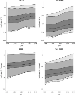
To illustrate the methodology a database drawn from World Bank was used that consists of the GDP (Y) in million dollars (in 2010 current prices), the capital (K), the labour (L) and the energy (E), measured in Ktoe, for several countries. For some countries the data were long-standing and up to date but unfortunately for others, the data were of more recent origin or were severely unreliable.

Thus, the complete available dataset consists of data over the period 1995-2014 for 109 countries, 35 members of OECD and 74 non-OECD countries, creating a balanced panel of 2180 observations. The chosen time period not only covers a sufficiently long period but also allows us to examine countries productive performance over a large number of countries during different economic cycles covering periods of expansion (growth) and contraction (recession).

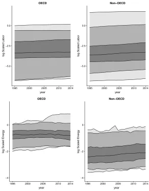
In this study the labor force was captured by the total hours worked by employees. The physical capital was estimated from gross fixed capital formation in million dollars (in 2010 current prices) using the perpetual inventory method with a depreciation rate of 10%, following, for example, King and Levine (1994). All variables were scaled with respect to the values of USA in 1995, year which was selected as the reference year. The time evolution of the four scaled variables across countries in a log-scale are presented in Figures 1 and 2. The central line presents the median while the far out lines present the max and min values for each year. The inner lines, defining the dark grey region, present the first and the third quartiles while the remaining lines, defining the light gray, present the upper 2.5% and 97.5% percentile points for each year.

coun-−10.0 −7.5 −5.0 −2.5 0.0

1995 2000 2005 2010 2014

year

log Scaled GPD

OECD

−10.0 −7.5 −5.0 −2.5 0.0

1995 2000 2005 2010 2014

year

log Scaled GPD

Non−OECD

−12 −8 −4 0

1995 2000 2005 2010 2014 year

log Scaled G. F

. Capital

OECD

−12 −8 −4 0

1995 2000 2005 2010 2014 year

log Scaled G. F

. Capital

Non−OECD

−5.0 −2.5 0.0

1995 2000 2005 2010 2014

year

log Scaled Labor

OECD

−5.0 −2.5 0.0

1995 2000 2005 2010 2014

year

log Scaled Labor

Non−OECD

−4 −2 0

1995 2000 2005 2010 2014

year

log Scaled Energy

OECD

−4 −2 0

1995 2000 2005 2010 2014

year

log Scaled Energy

Non−OECD

tries seems to consume a significant larger amount of energy since their third quartile is almost at the same level with the 97.5% percentile points of the non-OECD countries.

In the rest of this section, the Bayesian stochastic frontier model along with the proposed metafrontier stochastic model are presented. Table 1 summarizes the sample statistics of the countries data including the inputs and outputs for each group.

5.1

Frontier models for the two distinct group of countries

The empirical specification of the GDP in million dollars (in 2010 current prices) func-tion for each group of countries (OECD and non-OECD) was defined as followed

lnYit(j)=β0(j)+β1(j)Kit(j)+β2(j)Lit(j)+β3(j)Eit(j)+β4(j)t+vit(j)−uit(j), (11) for t=0, . . . ,19, i=1, . . . ,nj,j=1,2,whereYit(j)denotes the scaled, as described earlier, GDP in million dollars (in 2010 current prices) of thei−thcountry in the j−th group (j=1 refers to OECD countries and j=2 to non-OECD) at yeart(year 1995 was set ast=0) andK_it(j),L_it(j)andE_it(j)the corresponding scaled gross fixed capital formation (K), labor (L) and energy (E) respectively. A time trend was also included in the model, in order to obtain some temporal changes. Theβ(j)present the parameter vectors for the two groups while the unobservable random errors are assumed indepen-dent, normally distributed withv_it(j)∼N(0,σ2

v_(j))anduit(j)are assumed to follow an exponential distribution with parameterλ_u(j).

Since we wanted to tested our proposed method using as little as possible prior in-formation the non-informative priorsGamma(2,1/2)were chosen forσ−2

v andλu. For the regression parameters the following again non-informative priorβ∼N_k+1(0,104I)

was assigned.

For each group, the proposed MCMC algorithm was ran for a total of 200,000 iterations and the first 60,000 iterations discarded as burn-in. The trace plots (left) and kernel-smoothed estimates of the marginal posterior distributions (right) of some of the model’s parameters are presented in Figure 3. The plots present the marginal posterior distributions of the model’s parametersβ_0(j),β_1(j)andβ_2(j)for j=1 (OECD countries). In addition, some descriptive statistics for their posterior distributions (for both groups) are presented in Table 1.

Figure 3: The trace (left plots) and kernel-smoothed estimates of the marginal posterior distributions (right plots) of the model’s parameters β_0(j), β_1(j) and β_2(j) for j=1 (OECD countries).

Table 1: Descriptive statistics for the posterior distributions of the parameters of the frontier models (OECD countries - upper half, non-OECD countries - lower half).

Mean SD 2.5% Q1 Median Q3 97.5%

OECD

β0(1) -0.20550 0.047246 -0.29713 -0.23760 -0.20592 -0.17380 -0.11232

β1(1) 0.29602 0.009495 0.27740 0.28961 0.29611 0.30246 0.31440

β2(1) 0.66387 0.009329 0.64578 0.65753 0.66386 0.67015 0.68203

β3(1) 0.23878 0.015776 0.20800 0.22809 0.23883 0.24951 0.26943

β4(1) 0.01337 0.001634 0.01017 0.01227 0.01338 0.01448 0.01657

σ2

v₍₁₎ 0.09053 0.005190 0.08062 0.08696 0.09045 0.09403 0.10083

λu(1) 8.58404 1.416350 6.47614 7.57914 8.35415 9.34479 12.00389

non-OECD

β0(2) 0.03631 0.041242 -0.044666 0.008486 0.03653 0.06416 0.11662

β1(2) 0.24284 0.018576 0.206094 0.230523 0.24288 0.25508 0.27968

β2(2) 0.74136 0.016173 0.709327 0.730637 0.74131 0.75206 0.77329

β3(2) 0.17777 0.026575 0.125734 0.159862 0.17776 0.19564 0.22983

β4(2) 0.01198 0.001893 0.008264 0.010707 0.01199 0.01326 0.01569

σ2

v₍₂₎ 0.04720 0.004800 0.038276 0.043869 0.04701 0.05037 0.05705

1995 1997 19992001 20032005 2007 20092011 2013

0.0

0.2

0.4

0.6

0.8

1.0

TE

USA

1995 1997 19992001 20032005 2007 20092011 2013

0.0

0.2

0.4

0.6

0.8

1.0

TE

China

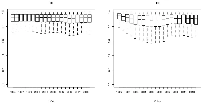
Figure 4: The boxplots of the posterior distributions of the technical efficiencies for the two leading economies of each group, namely the USA (left plot) and China (right plot) for all the years in the study.

5.1.1 Technical efficiencies results for the estimated frontiers

Since for each iteration of the MCMC algorithmuits are sampled from their full condi-tional posterior distribution for eachi,t and jone can obtain the descriptive statistics or the kernel-smoothed estimates of their posterior distributions, or equivalently for the Technical Efficiencies defined as

T E_it(j)=e−uit(j)_.

The boxplots of the posterior distributions are presented in Figure 4 of the technical efficiencies for the two leading economies of each group, namely the USA (OECD country) and China (non-OECD country) for all the years in the study. The USA seems to present a relative stable performance close to the group frontier presenting a small decrease just after 2008. On the other hand, China presents a more unstable behavior. Initially, the technical efficiency of China seems to decline and to reach its minimum around 2003 before it starts to slowly increase and stabilize after 2008. Comparing the level of the inefficiency of these two countries with respect to their frontier one can say that both economies perform relative close to their frontier model with USA to be the country that constantly performs better with respect to other countries in their group.

Table 2: The top and the last five countries’ efficiency scores under the technology fron-tier for each group (left panels) and the metatechnology fronfron-tier (right panel) based the mean value of the median of the posterior distributions in each year for each country.

OECD countries T E non-OECD countries T E Global technology T EMF

Champions Ireland 0.9462 Nigeria 0.9606 Italy 0.9088 United Kingdom 0.9455 Cuba 0.9499 Ireland 0.9029 Norway 0.9449 Sudan 0.9497 United Kingdom 0.9018 Luxembourg 0.9449 Saudi Arabia 0.9458 Switzerland 0.9017 Canada 0.9350 Uruguay 0.9432 Denmark 0.8962 Laggards Estonia 0.8521 Malaysia 0.8749 Singapore 0.7079 Slovak Republic 0.8201 Mongolia 0.8703 Malaysia 0.6954 Japan 0.7892 Nepal 0.8670 Korea, Rep. 0.6919 Czech Republic 0.7846 Ukraine 0.8152 Ukraine 0.6727 Korea, Rep. 0.7414 Thailand 0.7965 Thailand 0.6359

second, smaller, mode presents actually a single, outlier country). For the non-OECD countries there are several years, for example 1996, 2009 and the last two 2013 and 2014, that a clear bimodal behavior is observed.

Apart from that, the plots reveal a significant dispersion in 2005 and 2010 for the OECD countries. The measurements of 2005 can be interpret as creating an additive outlier behavior which has no latter affects. On the other hand, the measurements regarding 2010 seems to reflect an innovative outlier behavior in that year that seems to affect the subsequent years.

In order to observe in detail the changes that occur in the top and bottom ranked countries regarding their performance the mean value of the 20 posterior medians (one of each year) was calculated for each country. Although the median of the technical efficiency scores is only an indicative measure of the countries’ performance, their mean value can still provide an overall index of the performance of each country.

The first two panels in Table 2 show the top and last 5 countries under the tech-nology frontier for each group. Ireland, United Kingdom, Norway, Luxemburg and Canada consist the top five countries for the OECD frontier while Estonia, Japan, Slo-vak Republic, Czech Republic and Korea Republic consist the last five countries group. Regarding the non-OECD technological frontier, Saudi Arabia, Sudan, Cuba, Uruguay and Nigeria consist the champions group while Malaysia, Mongolia,Nepal, Ukraine and Thailand perform worst. The data concerning the metatechnology frontier pre-sented in the right panel of Table 2 are discussed in the following subsection.

5.2

Metafrontier model

As presented earlier a multivariate normal distribution is a natural choice forβM_{, the} parameter vector for the metafrontier model. Following the steps described in Section 4.1 one can obtain the following meanµ_βM and variance-covariance matrixΣofβM:

Σ₌₁₀−5_·



    

393.3035 37.0860 −3.4969 79.7091 −7.3321 37.0860 43.5219 −35.2888 43.2678 1.7793

−3.4969 −35.2888 34.8619 −38.8513 −1.9585

79.7091 43.2678 −38.8513 95.5108 1.8227 7.3321 1.7793 −1.9585 1.8227 0.6252



    

Figure 6 presents the time evolution of the technical efficiency with respect to the metafrontier (TEMF) of all countries. More specifically, the time evolution of TEMF is demonstrated by the kernel-smoothed estimates of the distribution of the medians of the technical efficiency with respect to the metafrontier of all countries determined by their posterior distributions. The light blue curves present the OECD countries and the grey curves the non-OECD countries. The distributions of the medians of the TEFM indicates a different picture compared with the technical efficiency with respect to the group frontier.

Both groups experience important dispersions and present significant heterogene-ity resulting to multimodal, left skewed distributions reflecting significant differences not only between the two groups but also within groups. The latter differences reflect the large dispersion of the technology gap ratios (TGR) , due to country-specific envi-ronments that is usually used to identify technological differentials with respect to the global meta-technology Battese et al. (2004); ODonnell et al. (2008), (Tsekouras et al., 2016, 2017).

In Figure 7 is presented the chronological change of the TGR for the OECD (left plot) and the non-OECD (right plot) countries. The central line presents the median while the far out lines present the max and min values for each year. The inner lines, defining the dark gray region, present the first and the third quartiles while the remain-ing lines, definremain-ing the light gray, present the upper 2.5% and 97.5% percentile points for each year. One of the interesting things to note in these plots is the relative large dis-persion of the TGR in each group which explains, as mentioned earlier, the significant differences of the TEFM within the two groups (see Figure 6).

Additional features of the plots in Figure 7 that are worth mentioning are the dif-ferent level of the TGR values in the two groups and the completely difdif-ferent trend of TGR which highlights especially in the last years the significant different values of the TGR between the two groups. the different trends denote a diverging rather a converg-ing behaviour of the two groups which in its turn indicates the increasconverg-ing technology gap between the two groups.

0.7 0.8 0.9 1.0

1995 2000 2005 2010 2014

year

TGR

OECD

0.7 0.8 0.9 1.0

1995 2000 2005 2010 2014

year

TGR

Non−OECD

Figure 7: The chronological change of the technology gap ratio (TGR) for the OECD (left plot) and the non-OECD (right plot) countries. The central line presents the me-dian while the far out lines present the max and min values for each year. The inner lines, defining the dark gray region, present the first and the third quartiles while the remaining lines, defining the light gray, present the upper 2.5% and 97.5% percentile points for each year.

opportunities Reichstein and Salter (2006) revealing non significant incoming spillover effects Tsekouras et al. (2016).

The out-performance of the OECD countries compared with the non-OECD coun-tries and the increasing technology gap between the two groups is clearly demon-strated in the boxplots of the posterior distributions of the TEMF for the two leading economies of each group, namely the USA and China for all the years in the study presented in Figure 8. It is interesting to note that even if the two countries are very close to their group frontier (see Figure 4), presenting non significant or small changes, especially China, their posterior distributions of the TEMF reveal other characteristics. Firstly, the posterior distribution of the TEMF of China takes significant smaller values compared with them of USA. Secondly, there is a clear different trend between the values of the TEMF between the two countries even if the decreasing trend of China seems to be slower after 2009. These findings reflects the weakness of China to take full advantage of the strong characteristics of its economy, as for example its large labor force (see the upper/maximum line of the upper right in Figure 2) which actual present the labor force if China.

1995 1997 19992001 20032005 2007 20092011 2013

0.0

0.2

0.4

0.6

0.8

1.0

TEMF

USA

1995 1997 19992001 20032005 2007 20092011 2013

0.0

0.2

0.4

0.6

0.8

1.0

TEMF

China

Figure 8: The boxplots of the posterior distributions of the technical efficiencies with respect to to the metafrontier for the two leading economies of each group, namely the USA (left plot) and China (right plot) for all the years in the study.

6

Concluding remarks

Heterogeneity exerts a multifaceted impact on countries’ performance and growth and it is closely related with their technology gap and spillover effects. The quantification of the technology gap is achieved through the adoption of a metafrontier framework. This approach has been applied broadly to DEA and SFA model across several dis-ciplines to account for. However, the literature argues on statistical properties of the metafrontier production function based on the second stage of linear programming of calculation.

This study is the first that propose a metatechnology production function under a Bayesian perspective to compare efficiencies of two distinct groups (OECD vs non-OECD countries). This aspect represents an essential contribution, since the literature lack evidence on Bayesian measures of technology gaps and on countries’ productive efficiency differentials. Moreover, the focus on technology gaps is crucial since it con-siders as an indicator of the technological level of each country but also reveal the degree of technological complexity of learning, the level of innovation and openness and the absorptive capabilities of the national economies. For the purpose of our em-pirical study we concentrate our efforts on a dataset consisting of 109 countries for a 20-year period from 1995-2014.

het-erogeneity and make clear countries’ idiosyncrasies and specificities. Furthermore, our specific finding underline the role of unsimilar competitiveness level, openness of their economies, innovation performance and specific idiosyncrasies regarding the institu-tional, economic and technological environment that each country operates.

We emphasize that we have merely show a model specification that can be extended in other more complex models such as translog. Although, this extensions may not be so straightforward as it may require further research due to slow convergence of the MCMCM algorithm due to the severe multicolinearity of the explanatory variables in such models. Finally, further research is required to test if the choice ofΣ_{is indeed the} optimal one and also to exploit its stochastic properties in order to compute credible regions for the metafrontier parameters.

References

D. Aigner, C.A.K. Lovell, and P. Schmidt. Formulation and estimation of stochastic frontier production function models.Journal of Econometrics, 6(1):21 – 37, 1977. C. Amsler, C.J. Odonnell, and . Schmidt. Stochastic metafrontiers. Econometric

Re-views, 36(6-9):1007–1020, 2017.

P. Bardhan and H. Lapan. Localized technical progress and transfer of technology and economic development.Journal of Economic Theory, December, 1973.

G.E. Battese and T.J Coelli. Frontier production functions, technical efficiency and panel data: with application to paddy farmers in india.

G.E. Battese and D.S.P. Rao. Technology gap, efficiency, and a stochastic metafrontier function.International Journal of Business and Economics, 1(2):87, 2002.

G.E. Battese, D.S.P. Rao, and C.J. O’donnell. A metafrontier production function for estimation of technical efficiencies and technology gaps for firms operating under different technologies.Journal of productivity analysis, 21(1):91–103, 2004. B. Casu, A. Ferrari, and T. Zhao. Regulatory reform and productivity change in indian

banking.Review of Economics and Statistics, 95(3):1066–1077, 2013.

Z. Chen, C.P. Barros, and M.R. Borges. A bayesian stochastic frontier analysis of chinese fossil-fuel electricity generation companies. Energy Economics, 48:136– 144, 2015.

G. Dosi, S. Lechevalier, and A. Secchi. Introduction: Interfirm heterogeneityna-ture, sources and consequences for industrial dynamics. Industrial and Corporate Change, 19(6):1867–1890, 2010.

J.E. Gal´an, H. Veiga, and M. P. Wiper. Dynamic effects in inefficiency: Evidence from the colombian banking sector. European Journal of Operational Research, 240(2): 562–571, 2015.

J.E. Griffin and M.F.J. Steel. Semiparametric bayesian inference for stochastic frontier models.Journal of econometrics, 123(1):121–152, 2004.

J.E. Griffin and M.F.J. Steel. Bayesian stochastic frontier analysis using winbugs. Jour-nal of Productivity AJour-nalysis, 27(3):163–176, Jun 2007.

G.E. Halkos and N.G. Tzeremes. Modelling the effect of national culture on multi-national banks’ performance: A conditional robust nonparametric frontier analysis. Economic modelling, 28(1-2):515–525, 2011.

Y. Hayami. Sources of agricultural productivity gap among selected countries. Ameri-can Journal of Agricultural Economics, 51(3):564–575, 1969.

Y. Hayami and V.W. Ruttan. Agricultural productivity differences among countries. The American economic review, pages 895–911, 1970.

Y. Hayami and V.W. Ruttan. Agricultural development: an international perspective. Baltimore, Md/London: The Johns Hopkins Press, 1971.

R.A. Horn and C.R. Johnson.Matrix Analysis. Cambridge University Press, 2 edition, 2012.

C.J. Huang, T. Huang, and N. Liu. A new approach to estimating the metafrontier pro-duction function based on a stochastic frontier framework. Journal of productivity Analysis, 42(3):241–254, 2014.

R.G King and R. Levine. Capital fundamentalism, economic development, and eco-nomic growth. InCarnegie-Rochester Conference Series on Public Policy, vol-ume 40, pages 259–292. Elsevier, 1994.

A. Kontolaimou, K. Kounetas, I. Mourtos, and K. Tsekouras. Technology gaps in european banking: Put the blame on inputs or outputs? Economic Modelling, 29(5): 1798–1808, 2012.

G. Koop, J. Osiewalski, and M.F.J. Steel. Bayesian efficiency analysis through indi-vidual effects: Hospital cost frontiers. Journal of Econometrics, 76(1-2):77–105, 1997.

K. Kounetas, I. Mourtos, and K. Tsekouras. Efficiency decompositions for heteroge-neous technologies. European Journal of Operational Research, 199(1):209–218, 2009.

W. Meeusen and J. van den Broeck. Efficiency Estimation from Cobb-Douglas Pro-duction Functions with Composed Error. International Economic Review, 18(2): 435–444, 1977.

A. M¨uller. Stochastic ordering of multivariate normal distributions. Annals of the Institute of Statistical Mathematics, 53(3):567–575, Sep 2001.

R.R. Nelson. An evolutionary theory of economic change. harvard university press, 2009.

C.J. ODonnell, D.S.P. Rao, and G.E. Battese. Metafrontier frameworks for the study of firm-level efficiencies and technology ratios. Empirical economics, 34(2):231–255, 2008.

T. Reichstein and A. Salter. Investigating the sources of process innovation among uk manufacturing firms.Industrial and Corporate change, 15(4):653–682, 2006. B.M. Tabak and P.L. Tecles. Estimating a bayesian stochastic frontier for the indian

banking system. International Journal of Production Economics, 125(1):96–110, 2010.

K. Tsekouras, N. Chatzistamoulou, K. Kounetas, and David C. Broadstock. Spillovers, path dependence and the productive performance of european transportation sectors in the presence of technology heterogeneity. Technological Forecasting and Social Change, 102:261–274, 2016.

K. Tsekouras, N. Chatzistamoulou, and K. Kounetas. Productive performance, tech-nology heterogeneity and hierarchies: Who to compare with whom. International Journal of Production Economics, 193:465–478, 2017.

E.G. Tsionas. Stochastic frontier models with random coefficients.Journal of Applied Econometrics, 17(2):127–147, 2002.