Munich Personal RePEc Archive
Growth: Scale or Market-Size Effects?
Chu, Angus C. and Cozzi, Guido
Fudan University, University of St. Gallen
August 2018
Growth: Scale or Market-Size E¤ects?
Angus C. Chu
Guido Cozzi
January 2019
Abstract
Is the supply of researchers or the demand for technologies more important for innovation? The supply of research labor captures a scale e¤ect, whereas the demand from production labor for technologies captures a market-size e¤ect. We …nd that both the scale e¤ect and the market-size e¤ect are important for innovation and their relative importance depends on R&D labor intensity. We collect data on R&D labor intensity and …nd that it varies signi…cantly across countries.
JEL classi…cation: O30, O40
Keywords: innovation, economic growth, scale e¤ects, market-size e¤ects
1
Introduction
In an in‡uential study, Jones (1995) shows that the R&D-based growth model features a scale e¤ect, which implies that a larger labor force causes a higher growth rate of technologies. Intuitively, with a larger labor force, there is more labor for R&D. Acemoglu (2002) shows that the R&D-based growth model also features a market-size e¤ect under which the growth rate of technologies is increasing in the amount of labor that uses the technologies. Therefore, the scale e¤ect and the market-size e¤ect are closely related. Acemoglu (2002) writes, "[s]ince the scale e¤ect is related to the market size e¤ect [...], one might wonder whether, once we remove the scale e¤ect, the market size e¤ect will also disappear."
This study disentangles the scale e¤ect and the market-size e¤ect. The supply of research labor determines the scale e¤ect, whereas the demand from production labor for technologies determines the market-size e¤ect. In a Schumpeterian growth model that features both lab-equipment R&D and knowledge-driven R&D, we …nd that the growth rate of technologies is generally increasing in both research labor and production labor. Therefore, both the scale e¤ect and the market-size e¤ect matter to innovation. However, their relative importance depends on the relative intensity of lab-equipment R&D and knowledge-driven R&D. Under knowledge-driven R&D that uses research labor as input, only the scale e¤ect matters to innovation. Under lab-equipment R&D that uses …nal good as input, only the market-size e¤ect matters to innovation. In general, the importance of the scale e¤ect relative to the market-size e¤ect is increasing in R&D labor intensity in the innovation process. Extending our analysis to a semi-endogenous growth model, we …nd that the scale e¤ect and the market-size e¤ect are still present but a¤ect the long-run level of technologies, instead of the long-run growth rate of technologies. Finally, we collect data on R&D labor intensity and …nd that it varies signi…cantly across countries.
This study relates to the literature on innovation and economic growth. Romer (1990) develops the seminal R&D-based growth model in which new products drive innovation. Segerstrom et al. (1990), Grossman and Helpman (1991a) and Aghion and Howitt (1992) develop the Schumpeterian model in which higher-quality products drive innovation. Jones (1999) shows that these seminal studies feature scale e¤ects and discusses two approaches of removing them. The semi-endogenous growth model originates from Jones (1995),1 whereas
the second-generation model originates from Smulders and van de Klundert (1995), Peretto (1998, 1999) and Howitt (1999) in which the market size of …rms is of fundamental impor-tance. Our analysis relates to this literature, which shows how the market-size dynamics at the …rm level is able to eliminate the scale e¤ect at the aggregate level.2 Acemoglu (2002)
de-velops a model of directed technical change and shows that the market-size e¤ect exists even without the scale e¤ect on growth; however, his formulation maintains the scale e¤ect on level. Our study complements Acemoglu (2002) by showing the di¤erent determinants of the scale and market-size e¤ects and the importance of the relative intensity of two conventional R&D speci…cations.
1See also Grossman and Helpman (1991b, p. 75-76) who anticipated the semi-endogenous growth model. 2See Laincz and Peretto (2006) and Peretto (2018) for empirical and theoretical justi…cations for the
2
A Schumpeterian growth model
We consider the Schumpeterian model. Previous studies often assume that the R&D sector uses either research labor (i.e., knowledge-driven R&D) or …nal good (i.e., lab-equipment R&D). We specify a generalized R&D process that uses both research labor and …nal good.
2.1
Household
The representative household has the following utility function:
U =
Z 1
0
e tlnc
tdt, (1)
where ct denotes consumption at time t and the parameter > 0 is the discount rate. The household exogenously supplies m units of manufacturing labor ands units of research labor. Research labors is the supply of an input for innovation and captures the scale e¤ect. Production labormuses invented technologies and determines the market size of innovation. The household maximizes utility subject to the following asset-accumulation equation:
_
at=rtat+wm;tm+ws;ts ct. (2)
at is the real value of assets (i.e., the share of monopolistic …rms). rt is the real interest rate.
wm;t and ws;t are respectively the real wage rates ofm and s. Dynamic optimization yields
_ ct
ct
=rt . (3)
2.2
Final good
Competitive …rms produce …nal good yt using the following Cobb-Douglas aggregator:
yt= exp
Z 1
0
lnxt(i)di , (4)
where xt(i) is intermediate good i 2 [0;1]. Pro…t maximization yields the following condi-tional demand function for xt(i):
xt(i) =
yt
pt(i)
, (5)
2.3
Intermediate goods
There is a unit continuum of monopolistic industries producing di¤erentiated intermediate goods. The production function of the industry leader in industry i2[0;1] is
xt(i) =zqt(i)mt(i), (6)
where the parameterz >1is the quality step size,qt(i)is the number of quality improvements that have occurred in industry i as of timet, and mt(i)is manufacturing labor employed in industry i. Given the productivity level zqt(i), the marginal cost of the leader in industry i
is wm;t=zqt(i). The pro…t-maximizing monopolistic price is
pt(i) =
wm;t
zqt(i), (7)
where the markup 2 (1; z] is a policy parameter determined by the government.3 The
wage payment is
wm;tmt(i) =
1
pt(i)xt(i) =
1
yt, (8)
and the monopolistic pro…t is
t(i) =pt(i)xt(i) wm;tmt(i) =
1
yt. (9)
2.4
R&D
Equation (9) shows that t(i) = t. Therefore, the value of inventions is the same across industries such that vt(i) = vt.4 The no-arbitrage condition that determines vt is
rt=
t+ _vt tvt
vt
, (10)
which states that the rate of return on vt is equal to rt. The return on vt is the sum of monopolistic pro…t t, capital gain v_t and expected capital loss tvt, where t is the arrival rate of innovation.5
Competitive entrepreneurs maximize pro…t by recruiting research labor st and devoting
Rt units of …nal good to perform innovation. The arrival rate of innovation is
t ='(st)1
Rt
Zt
, (11)
3Grossman and Helpman (1991a) and Aghion and Howitt (1992) assume that the markup is equal to the
quality step sizez, due to limit pricing between current and previous quality leaders. Here we follow Evans
et al. (2003) to consider price regulation under which the regulated markup ratio is 2(1; z].
4We follow the standard approach in the literature to focus on the symmetric equilibrium. See Cozziet
al. (2007) for a theoretical justi…cation for the symmetric equilibrium to be the unique rational-expectation equilibrium in the Schumpeterian model.
5When the next innovation occurs, the previous technology becomes obsolete. This is known as the Arrow
where' >0is a productivity parameter andZt denotes aggregate technology. The parame-ter 2[0;1]is the intensity of …nal good relative to research labor in the innovation process. Knowledge-driven R&D is captured by = 0, whereas lab-equipment R&D is captured by
= 1. The …rst-order conditions forfst; Rtg are(1 ) tvt=ws;tst and
tvt=Rt, 's1
Rt
Zt
1
vt
Zt
= 1, (12)
which uses (11) and the resource constraint st=s.
2.5
Economic growth
Aggregate technologyZt is de…ned as
Zt exp
Z 1 0
qt(i)dilnz = exp
Z t
0
!d!lnz , (13)
which uses the law of large numbers. Di¤erentiating the log ofZtwith respect to time yields the growth rate of technology given by
gt
_ Zt
Zt
= tlnz. (14)
Substituting (6) into (4) yields the aggregate production function given by
yt= exp
Z 1
0
qt(i)dilnz+
Z 1
0
lnmt(i)di =Ztm. (15)
Thus, the growth rate of output yt is also gt, which is determined by t as shown in (14). From (3) and (10), the balanced-growth value of an invention is
vt= t
+ =
1 Ztm
+ , (16)
which uses (9) and (15). Equation (16) shows that vt is increasing in production labor m, capturing the market-size e¤ect in Acemoglu (2002). Substituting (16) into (12) yields
= 's1 Rt Zt
1
1
m . (17)
Substituting the resource constraint st=s into the arrival rate of innovation in (11) yields
='s1 Rt Zt
, (18)
where Rt is still endogenous. Combining (17) and (18) yields
which determines the unique steady-state equilibrium .
Equation (19) shows that the arrival rate of innovation is increasing in production labor m (i.e., the market-size e¤ect) and research labor s (i.e., the scale e¤ect). Therefore, the equilibrium growth rate g in (14) is also increasing in m and s. The complementarity betweenmandsin (19) implies that how country size a¤ects growth depends on the product ofmands. For example, a large country with a low innovation capacitys(e.g., China in the early reform period) cannot achieve high growth from innovation by simply having a large market size m.
Proposition 1 Economic growth is increasing in production labor m (i.e., the market-size e¤ect) and research labor s (i.e., the scale e¤ect).
Considering a zero discount rate !0, we simplify (19) to
lim
!0 =
1
's1 m . (20)
Substituting (20) into (14) yields
lim
!0 g =
1
's1 m lnz, (21)
which shows that the importance of the market-size e¤ect m relative to the scale e¤ect s
on growth is increasing in the intensity of …nal good relative to research labor in the innovation process. Equation (19) shows that this result is robust to >0.6 Intuitively, as
increases, R&D spending Rt becomes more important for innovation relative to research labor st; consequently, the market-size e¤ect, which determines the value of inventions, becomes more important relative to the scale e¤ect in determining innovation. Proposition 2 summarizes this result.
Proposition 2 The importance of the market-size e¤ect m relative to the scale e¤ect s on economic growth is increasing in the intensity of …nal good relative to research labor in the innovation process.
Finally, we consider knowledge-driven R&D given by = 0 and lab-equipment R&D given by = 1. Under knowledge-driven R&D, the arrival rate of innovation is KD ='s
and the growth rate of technology is gKD = 'slnz. Therefore, only the scale e¤ect s matters under knowledge-driven R&D because innovation is solely determined by the supply of research labor in this case.7 Under lab-equipment R&D, the arrival rate of innovation is
LE
='m( 1)= , and the growth rate of technologies isgLE = LE
lnz. Therefore, only
6One can apply the approximationln(X) X 1to (19) to show that@ =@m and@ =@s 1 . 7This result is robust to allowingsto be allocated between researchs
r and productionsx. For example,
the market-size e¤ectmmatters under lab-equipment R&D because innovation is determined by the demand for technologies in this case.8 Proposition 3 summarizes these results.
Proposition 3 Under knowledge-driven R&D, only the scale e¤ectsmatters to innovation. Under lab-equipment R&D, only the market-size e¤ect m matters to innovation.
3
A scale-invariant Schumpeterian growth model
In this section, we allow for population growth and convert the model into a semi-endogenous growth model to examine its implications. In this case, we assume that research labor is
st sLtand production labor ismt mLt, where s+m 1and populationLt increases at an exogenous growth raten > 0. Then, we modify the innovation process in (11) as follows:
t=
'(st)1
Zt
Rt
Zt
, (22)
where the parameter > 0 and the new term Zt capture an increasing-di¢culty e¤ect of R&D similar to Segerstrom (1998). The rest of the model is the same as in Section 2. We will show thatRt=Zt is proportional tomtand increases at the raten in the long run. Therefore,
(st)1 (Rt=Zt) also increases at the raten. Then, a steady-state arrival rate of innovation requires that Zt also grows at the rate n in the long run. Therefore, the long-run growth rate of aggregate technologyZt isg =n= , and the steady-state arrival rate of innovation is
=g=lnz =n=( lnz).9
Substituting (16) into tvt=Rt yields
Rt
Zt
= 1
+ mt, (23)
which shows that Rt=Zt is proportional to mt in the long run. Substituting (23) into (22) yields the long-run level of technology (per capita) as follows:
Zt
Lt
= '(st)
1 (m
t)
Lt
1
+ =
's1 m 1
+ , (24)
where = n=( lnz) is determined by exogenous parameters. Equation (24) shows that the long-run level of technology is increasing in the market-size e¤ect m and the scale e¤ect
s. Furthermore, the relative importance of the market-size e¤ect m and the scale e¤ect s
8If we assume thatscan be allocated to productions
xand specifyxt(i) =zqt(i)[mt(i)] [sx;t(i)]1 , then
gLE= ['m s1 ( 1)= ] lnz. Although innovation is also determined bysin this case, its e¤ect works
through the market size (i.e., the demand from production laborsx=sfor technologies).
9Alternatively, one can achieve long-run endogenous growth despite population growth by replacing Z
t
in (22) withLt, which captures a dilution e¤ect in the spirit of the second-generation model; see Laincz and
Peretto (2006). In this case, (19) remains the same except thats1 m is given by(s
t=Lt)1 (mt=Lt) . In
on innovation is determined by the relative intensity of …nal good and research labor in innovation. Under knowledge-driven R&D (i.e., = 0), only the scale e¤ect s matters to innovation. Under lab-equipment R&D (i.e., = 1), only the market-size e¤ectmmatters to innovation. All these results are the same as before, except the e¤ect on innovation is re‡ected in the long-run level of technology instead of the long-run growth rate of technology.10
3.1
Labor allocation
In this section, we extend the semi-endogenous growth model by allowing for labor allocation ins to ensure the robustness of our results whens can be allocated between researchsr and productionsx. Speci…cally, we modify (6) as follows:
xt(i) =zqt(i)[mt(i)] [sx;t(i)]1 , (25) where 2(0;1). In Appendix B, we derive the long-run level of technology as
Zt
Lt
= '(sr;t)
1 (s
x;t) (1 )(mt)
Lt
1
+ =
's1 m
, (26)
where =n=( lnz)and the composite parameter is de…ned as
1 1
1
( 1) +
h
1 + 11 (+1)i1
.
Equation (26) shows that technologyZ =Ltis increasing in the market-size e¤ect mand the scale e¤ect s. The importance of m relative to s is increasing in . The exponent on s is
1 = 1 + (1 ), where1 captures the scale e¤ect fromsrand (1 )captures
the market-size e¤ect from sx. Under knowledge-driven R&D (i.e., = 0), only the scale e¤ect s matters to technology because the market-size e¤ect m does not a¤ect R&D labor
sr. Under lab-equipment R&D (i.e., = 1), only the market-size e¤ect m s1 matters, where s1 captures the demand from production labor(s
x)1 for technologies.
4
Does R&D labor intensity vary across countries?
If we assume that R&D laborstand production labormtare mobile between the two sectors subject to st+mt = lt Lt where lt denotes labor force, then the wage rate is equalized between the two types of labor such that ws;t =wm;t = wt. In this case, we can construct
10In an earlier version, we also consider a hybrid model that features both endogenous growth and
R&D labor intensity 1 from data as follows:11
1 = wtst wtst+Rt
=
R&D share of labor z }| {
(st=lt)
(wtst+Rt)=yt
| {z }
R&D share of GDP
labor income/GDP z }| {
(wtlt=yt) . (27)
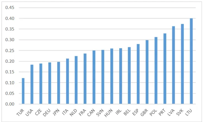
[image:10.612.129.484.237.449.2]Figure 1 shows that R&D labor intensity varies signi…cantly even across OECD countries. For example, the US has a relatively low R&D labor intensity suggesting that the market-size e¤ect is more vital for its innovation than the scale e¤ect, compared to a country like the UK which has a relatively high R&D labor intensity.
Figure 1: Average R&D labor intensity from 1996 to 2014
5
Conclusion
In this study, we …nd that both the supply of research labor that determines the scale e¤ect and the demand from production labor for technologies that determines the market-size e¤ect matter to innovation. Interestingly, the relative importance of these supply and demand factors depends on the relative intensity of lab-equipment R&D and knowledge-driven R&D in the innovation process. Therefore, this structural parameter has important empirical implications. For example, it determines whether an education policy that increases research labor at the expense of production labor stimulates or sti‡es economic growth. If the intensity of lab-equipment R&D is high relative to knowledge-driven R&D, then a policy that promotes apprenticeships, such as the European Alliance for Apprenticeships, may be more e¤ective in stimulating economic growth.
References
[1] Acemoglu, D., 2002. Directed technical change. Review of Economic Studies, 69, 781-809.
[2] Aghion, P., and Howitt, P., 1992. A model of growth through creative destruction. Econometrica, 60, 323-351.
[3] Chu, A., and Cozzi, G., 2018. Growth: Scale or market-size e¤ects? MPRA Paper No. 89710.
[4] Cozzi, G., 2007. The Arrow e¤ect under competitive R&D.The B.E. Journal of Macro-economics (Contributions), 7, Article 2.
[5] Cozzi, G., 2017. Endogenous growth, semi-endogenous growth... or both? A simple hybrid model. Economics Letters, 154, 28-30.
[6] Cozzi, G., Giordani, P., and Zamparelli, L., 2007. The refoundation of the symmetric equilibrium in Schumpeterian growth models. Journal of Economic Theory, 136, 788-797.
[7] Evans, L., Quigley, N., and Zhang, J., 2003. Optimal price regulation in a growth model with monopolistic suppliers of intermediate goods.Canadian Journal of Economics, 36, 463-474.
[8] Grossman, G., and Helpman, E., 1991a. Quality ladders in the theory of growth.Review of Economic Studies, 58, 43-61.
[9] Grossman, G., and Helpman, E., 1991b.Innovation and Growth in the Global Economy. The MIT Press.
[10] Howitt, P., 1999. Steady endogenous growth with population and R&D inputs growing. Journal of Political Economy, 107, 715-730.
[11] Jones, C., 1995. R&D-based models of economic growth.Journal of Political Economy, 103, 759-784.
[12] Jones, C., 1999. Growth: With or without scale e¤ects. American Economic Review, 89, 139-144.
[13] Laincz, C., and Peretto, P., 2006. Scale e¤ects in endogenous growth theory: An error of aggregation not speci…cation. Journal of Economic Growth, 11, 263-288.
[14] Peretto, P., 1998. Technological change and population growth. Journal of Economic Growth, 3, 283-311.
[15] Peretto, P., 1999. Cost reduction, entry, and the interdependence of market structure and economic growth. Journal of Monetary Economics, 43, 173-195.
[17] Romer, P., 1990. Endogenous technological change. Journal of Political Economy, 98, S71-S102.
[18] Segerstrom, P., 1998. Endogenous growth without scale e¤ects. American Economic Review, 88, 1290-1310.
[19] Segerstrom, P., Anant, T., and Dinopoulos, E., 1990. A Schumpeterian model of the product life cycle. American Economic Review, 80, 1077-91.
Appendix A: Second-generation model (not for publication)
In this appendix, we show that the dilution e¤ect mentioned in footnote 9 can be micro-founded in a second-generation model with both quality improvement and variety expansion. We modify the production function in (4) as
yt =Ntexp
1 Nt
Z Nt
0
lnxt(i)di , (A1)
where Nt is the endogenous mass of di¤erentiated intermediate goods. Following Howitt (2000), we specify the law of motion for Nt as
_
Nt = Lt, (A2) where > 0 is an exogenous parameter. A stationary N_t=Nt on the balanced growth path implies a stationary ratio Lt=Nt, which in turn implies that the long-run growth rate of Nt is also n. Therefore, Nt is proportional to Lt in the long run, such that Nt = Lt=n. If we use the parameter normalization =n, then Nt=Lt.
As for the rest of the model,ytin (5), (8) and (9) is replaced by yt=Nt. Furthermore, the resource constraints on production labor and research labor become
Z Nt
0
mt(i)di=mLt)mt(i) =
mLt
Nt
=m, (A3)
Z Nt
0
st(i)di=sLt )st(i) =
sLt
Nt
=s, (A4)
where the second set of equations in (A3) and (A4) applies symmetry and uses the long-run condition Nt=Lt. Aggregate technology in (13) becomes
Zt exp
1 Nt
Z Nt
0
qt(i)dilnz = exp
Z t
0
!d!lnz , (A5)
and the growth rate ofZt isgt= tlnz. Aggregate production function in (15) becomes
yt =Ntexp
1 Nt
Z Nt
0
qt(i)dilnz+
1 Nt
Z Nt
0
lnmt(i)di =ZtmLt, (A6)
where the last equality uses Nt=Lt. Therefore, the growth rate of yt is g+n= lnz+n. Substituting t(i) = [( 1)= ]yt=Nt into (10) yields (16).12 Finally, (17) and (18) are the same as before and give rise to the same steady-state equilibrium in (19), wherem and s
are now production labor and research labor per variety.
References
[1] Howitt, P., 2000. Endogenous growth and cross-country income di¤erences. American Economic Review, 90, 829-846.
12To obtain (16) in the second-generation model, we rede…ne utility in (1) such that the real interest rate
Appendix B: Labor allocation (not for publication)
In this appendix, we generalize the production function in (6) as follows:
xt(i) =zqt(i)[mt(i)] [sx;t(i)]1 . (B1) From cost minimization, the marginal cost of production for the leader in industryi is
M Ct(i) =
1 zqt(i)
wm;t ws;t
1
1
. (B2)
Given pt(i) = M Ct(i), the monopolistic pro…t and wage payments are respectively
t(i) =
1
pt(i)xt(i) =
1
yt, (B3)
wm;tmt(i) = pt(i)xt(i) = yt, (B4)
ws;tsx;t(i) =
1
pt(i)xt(i) =
1
yt. (B5) The arrival rate t of innovation is given by (22) with st replaced by sr;t. The …rst-order conditions for fsr;t; Rtg are
(1 ) tvt=ws;tsr;t, (B6)
tvt =Rt. (B7)
Substituting (B1) into (4) yields
yt=Zt(mt) (sx;t)1 . (B8) From (3) and (10), the balanced-growth value of an invention is
vt= t
+ =
1Zt(mt) (sx;t)1
+ , (B9)
where the second equality uses (B3) and (B8). Substituting (B9) into (B7) yields
Rt
Zt
= +
1
(mt) (sx;t)1 . (B10)
Substituting (B5) and (B9) into (B6) yields
sr;t
sx;t
= 1 1
( 1)
+ . (B11)
Substituting (B10) and (B11) into (22) yields
= '(sx;t)
1 (m t) Zt 1 1 1 ( 1)
+ , (B12)
which shows that a steady-state equilibrium requiresZt to grow at the raten. Substituting (B11) into sx;t+sr;t=st yields
st= 1 +
1 1
( 1)
+ sx;t. (B13)