Approximate multipliers for MAC

(1)

Approximate multipliers for MAC

Verstoep, B. (s1009966)

(2)

Abstract

Approximate computing techniques reduce the cost (in terms of among others area and power consumption) of computing units in exchange for a reduced accuracy. These techniques are not optimized for Multiply-Accumulate (MAC) processing elements. This leaves a lot of room for improvement as the integrator part of a MAC allows for error balancing.

(3)

Introduction

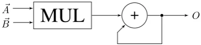
Multiply-Accumulate (MAC) circuits are a type of circuit that calculates the dot product of two input vec-tors. MAC circuits are widely used in many different applications. One use of MAC circuits is for example radio astronomy[1].

Figure 1 shows a diagram of a MAC processing element. The elements of the two input vectors are multi-plied, and the results added together using an integrator. The output of the MAC is given in equation (1). HereO is the output of the MAC.M is the number of elements in the input vectors. An andBn are the nth elements of the input vectorsA~andB.~

~ A ~

[image:4.595.200.400.336.381.2]

B

MUL

+

O

Figure 1: MAC processing element diagram

O=A~·B~ = M

X

n=1

(An∗Bn) (1)

In this work the use of approximate computing techniques[2][3] is explored to reduce the cost, in terms of area for FPGA, while keeping the accuracy of the computation as high as possible. The multiplier of the MAC can be replaced by an approximate multiplier and the integrator can make use of approximate adders. In this work the adders will be kept accurate and the focus will lie on approximating the multipliers efficiently. The inputs are assumed to be uncorrelated. The goal is to find an approximate design of an 8 bit MAC processing element which has the lowest cost for a given quality or the best accuracy for a given cost. The cost considered is the area used on an FPGA.

(5)

Chapter 1 Approximate multipliers

In this chapter existing techniques for creating an approximate multiplier are introduced. Also the method to calculate the average error of a multiplier is discussed.

1.1 Creating a multiplier

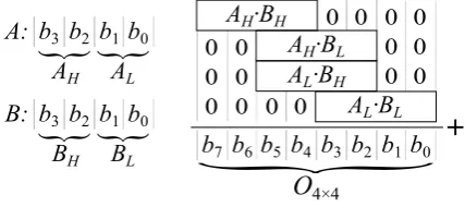
An existing technique of creating approximate multipliers is to make a small and efficient2×2 bit ap-proximate multiplier and use multiple of them to create a largern×nmultiplier[4]. To create a4×4bit multiplier, the two 4 bit inputs,AandB, are divided into two 2 bit parts each. These are calledAH,AL, BH andBL. TheH indicates the most significant part of the inputs andLthe least significant part. To calculate the 8 bit output of the4×4 bit multiplier,O4×4, the input parts will first be multiplied using 2×2bit multipliers. The 2 bit partial inputs fromAare then multiplied with the 2 bit partial inputs of Bin all possible combinations. The resulting four outputs are then shifted, where a more significant input means more shifting for the output. This process is shown in equation (1.1) and illustrated in Figure 1.1.

L 0

0 0

0 0 0

0 0 0 0 0

0 0

+

(6)

a factor of 4. For an×nmultiplier, wheren= 2k_{, there are}₄k−1_{of the}₂_×₂_{multipliers needed.}

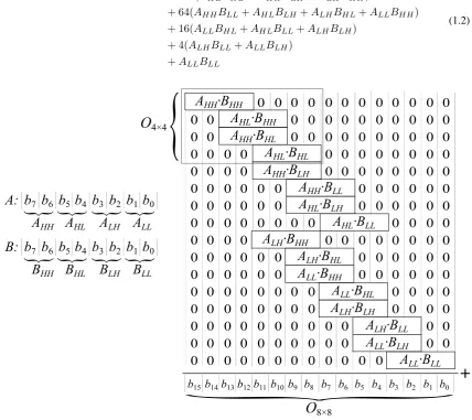
O8×8= 4096AHHBHH+ 1024(AHLBHH+AHHBHL)

+ 256(AHLBHL+AHHBLH+ALHBHH)

+ 64(AHHBLL+AHLBLH+ALHBHL+ALLBHH)

+ 16(ALLBHL+AHLBLL+ALHBLH)

₄

B:

{

B

HL

B

HH

_4×4

Figure 1.2: An8×8bit multiplier using2×2bit multiplier elements

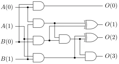
1.2 Existing

2 ×

2 bit multiplier elements

(7)

A(0)

A(1)

B(0)

B(1)

O(0)

O(1)

O(2)

[image:7.595.204.398.124.229.2]

O(3)

Figure 1.3: Accurate2×2bit multiplier design

Table 1.1: Accurate2×2multiplier design truth table

B A

00 01 10 11

00 0000 0000 0000 0000 01 0000 0001 0010 0011 10 0000 0010 0100 0110 11 0000 0011 0110 1001

A(0)

A(1)

B(0)

B(1)

O(0)

O(1)

O(2)

O(3)

(a)M1

A(0)

A(1)

B(0)

B(1)

O(0)

O(1)

O(2)

O(3)

(b)M2

Figure 1.4: Approximate2×2bit Multiplier Designs

Table 1.2: Approximate2×2multiplier designs truth tables (a) M1

B A

00 01 10 11

00 0000 0000 0000 0000 01 0000 0000 0010 0010

10 0000 0010 0100 0110 11 0000 0010 0110 1001

(b) M2

B A

00 01 10 11

(8)

1.3 Calculating the average error

A figure of the quality of an approximate multiplier can be the average error of the multiplier. To get the maximum quality, the average error should be as small as possible. The average error of the multiplier can be calculated by multiplying the probability of an error occurring with the weighted error magnitude. Here the weighted magnitude is the error magnitude of the2×2multiplier, multiplied with the shift due to the location of the2×2multiplier as shown in (1.2). Each of the 16 approximate2×2multipliers (for 8×8bit) has its own error probability and weighted magnitude. For example the multiplier calculating AHH∗BHHusingM2has a much bigger weighted error magnitude (|4096∗−2|= 8192) than for example ALLBLL(|1∗ −2|= 2). The probability of the error occuring at each multiplier is dependent on the input distribution. For a uniform distribution the probability of each input is equally likely and therefore the probability for en error in every multiplier usingM2is1/16which is the amount of errors divided by the number of (equally likely) options in the truth table in Figure 1.4(b). For other distributions, calculating the probability is much harder. For example with a normal distribution, if the probability for the highest numbers is much lower, the most significant bits of the input are more likely to be0 and therefore the probability of the2×2bit calculation being3∗3, where the error occurs forM2, is much lower.

To calculate the average error, the probability needs to be multiplied by the weighted magnitude of the error for each of the 16 multipliers and added up. This can be generalised for an×nmultiplier. This is shown in equation (1.3). HereEis the average error of the whole multiplier.Siis the shift of the output of the2×2multiplier seen in equation (1.2).Eiis the error magnitude andP(E)ithe probability of an error occuring for theith2×2multiplier.

E=

4k−1

X

i=1

(9)

Chapter 2 Approximate multipliers for MAC

There is a distinct difference between creating an approximate multiplier for a MAC as opposed to just an approximate multiplier in general. When calculating the outcome of a multiplication every result counts. It does not matter if the errors made are sometimes negative and sometimes positive. For a MAC however the multiplier gets followed up by an integrator which sums all the results of the multiplier. The individual multiplications do not matter as much as the end result of the addition. If in the multiplications sometimes a negative error is made and sometimes a positive error, the errors add up in the integrator and compensate eachother, resulting in a lower error of the total MAC operation.

2.1 Average error for MAC

To calculate the average error of the MAC, equations (1) and (2.1) are used to create equation (2.2). Note that equation (2.1) is a slight variation on equation (1.3). This is because for the calculation of the average error of a MAC the sign of the error does matter. Therefore the absolute operation is removed and the new variable is calledE0

O=A~·B~ = M

X

n=1

(An∗Bn) (1 revisited)

E0 ₌

4k−1

X

i=1

(Si∗Ei∗P(E)i) (2.1)

EM AC =

M X n=1 E0 = M X n=1

4k−1

X

i=1

(Si∗Ei∗P(E)i)

=M

4k−1

X

i=1

(Si∗Ei∗P(E)i)

(2.2)

Because the errors may cancel each other, the absolute value is taken after the addition of the errors of each of the2×2multipliers instead of before addition.

2.2 Error balancing methods

(10)

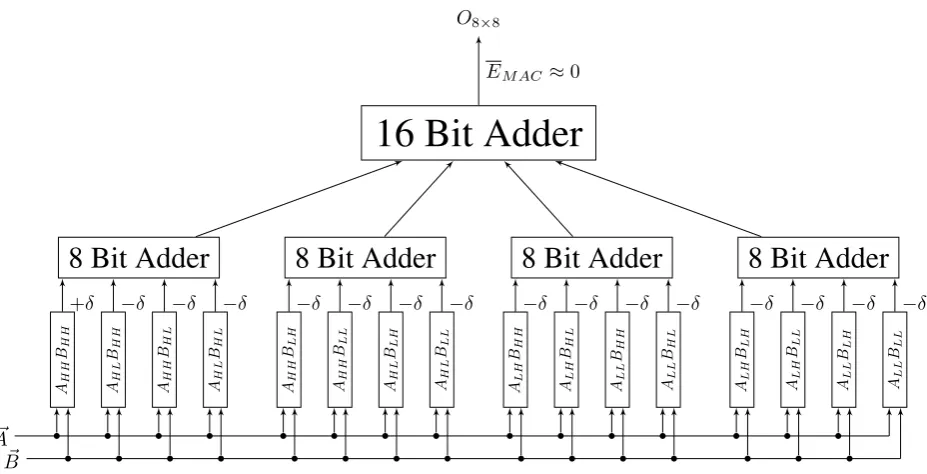
AH H BH H AH L BH H AH H BH L AH L BH L AH H BLH AH H BLL AH L BLH AH L BLL ALH BH H ALH BH L ALL BH H ALL BH L ALH BLH ALH BLL ALL BLH ALL BLL

8 Bit Adder

16 Bit Adder

+δ −δ −δ −δ −δ −δ −δ −δ −δ −δ −δ −δ −δ −δ −δ −δ O8×8

EM AC ≈0

[image:10.595.97.561.107.344.2]

~ A ~ B

Figure 2.1: Internal error balancing of an8×8bit multiplier

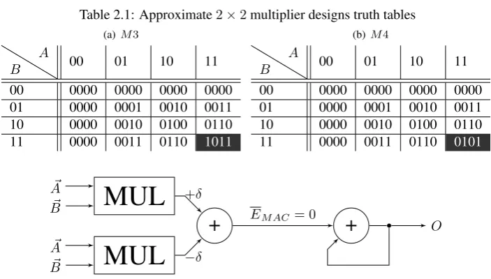
A(0) A(1) B(0) B(1) O(0) O(1) O(2) O(3) (a)M3 A(0) A(1) B(0) B(1) O(0) O(1) O(2) O(3)

(b)M4

Figure 2.2:2×2bit Multiplier Designs for error balancing purposes

An example is shown in Figure 2.1. The+δand−δare the errors of the2×2multiplier elements. +δ indicates an overall positive error and−δa negative error. For the purpose of creating a balanced multiplier two new2×2multipliers are introduced in Figure 2.2. Their truth tables can be found in Table 2.1.

M3in Figure 2.2(a) is a multiplier made to directly balanceM2. It has the same error probability but the opposite error magnitude. To more precisely balance the multiplier to get an average error closer to0, M4is introduced. The only difference between this multiplier andM2is that an OR-gate is replaced by an XOR-gate resulting in a larger error and simular area for FPGA as will be shown in chapter 3. These multipliers can used in conjunction with the ones introduced in chapter 1 to create a single set of 16 multi-pliers creating both negative and positive errors which cancel each other out as close to0as possible.

[image:10.595.104.501.390.516.2]

(11)

[image:11.595.124.476.112.312.2]

Table 2.1: Approximate2×2multiplier designs truth tables (a)M3

B A

00 01 10 11

00 0000 0000 0000 0000 01 0000 0001 0010 0011 10 0000 0010 0100 0110 11 0000 0011 0110 1011

(b)M4

B A

00 01 10 11

00 0000 0000 0000 0000 01 0000 0001 0010 0011 10 0000 0010 0100 0110 11 0000 0011 0110 0101

~ A ~

B

MUL

~ A ~

B

MUL

+

O

+δ

−δ

EM AC= 0

Figure 2.3: Two8×8bit multipliers used as mirror pair in a MAC

(12)

Chapter 3 Quality and computational cost analysis

In this chapter the methods of calculating the quality and computational cost of the designs is discussed. The quality is calculated using a Matlab model and the computational cost is calculated using Quartus.

3.1 Matlab model of a MAC

The code for the Matlab model of a MAC can be found in Appendix A. The model calculates the accurate and the approximate outcomes of a generated set of inputs.

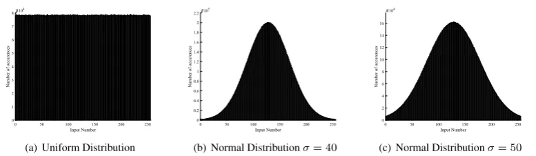
Three sets of random inputs with different input distributions are generated using Matlab. The inputs range from0to255(8 bit). The input vector size of the MAC,M, will be chosen as10000and the result of the MAC will be computed1000times. One input set is a uniform distribution, generated using the Matlab functionrandi. The other two sets are normal distributions with an average of128and a standard deviation of40and50respectively. The resulting distributions are shown in the histograms in Figure 3.1.

The accurate result of the MAC is calculated using the built-indotfunction of Matlab. The approxi-mate version is calculated by first separating the 8 bit inputs into the 2 bit inputs of each of the 162×2bit multiplier elements. Next, the accurate products of those 2 bit inputs are calculated. Dependent on which multiplier is used for which of the inputs, the 4 bit outputs are adjusted to include the errors. For example, for multiplierM2every9in the output is replaced with a7. The results are summed using equation (1.2) from chapter 2 to get the output of the total approximate multiplier and finally summed to get the result of the MAC.

0 50 100 150 200 250

Input Number 0

1 2 3 4 5 6 7 8

Number

of

occurences

#104

(a) Uniform Distribution

0 50 100 150 200 250 Input Number

0 0.2 0.4 0.6 0.8 1 1.2 1.4 1.6 1.8 2 2.2

Number of occurences

#105

(b) Normal Distributionσ= 40

0 50 100 150 200 250 Input Number

0 2 4 6 8 10 12 14 16

Number of occurences

#104

[image:12.595.109.498.565.678.2]

(c) Normal Distributionσ= 50

(13)

[image:13.595.96.514.135.225.2]

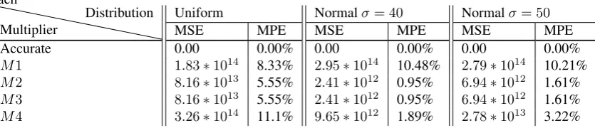
Table 3.1: MSE and MAE for different distributions for8×8MAC with a single type of2×2multiplier each

Multiplier

Distribution Uniform Normalσ= 40 Normalσ= 50

MSE MPE MSE MPE MSE MPE

Accurate 0.00 0.00% 0.00 0.00% 0.00 0.00%

M1 1.83∗1014 8.33% 2.95∗1014 10.48% 2.79∗1014 10.21% M2 8.16∗1013 5.55% 2.41∗1012 0.95% 6.94∗1012 1.61% M3 8.16∗1013 5.55% 2.41∗1012 0.95% 6.94∗1012 1.61% M4 3.26∗1014 11.1% 9.65∗1012 1.89% 2.78∗1013 3.22%

3.2 Quality analysis using the Matlab model

The resulting MAC outputs are compared to get a figure of quality. A commenly used metric of quality is the Mean Square Error[6][7]. The Mean Square Error (MSE) is calculated by calculating the square of the difference (or error) between each of the1000accurate and approximate MAC results. That result is divided by the total amount of MAC results, in this case1000, to get the mean. This is shown in equa-tion (3.1). Hereαis the result of the accurate MAC calculation andβ the result of the approximate.nis the amount of calculations.

MSE= (α1−β1) 2_{+ (}_α

2−β2)2. . .+ (αn−βn)2

n (3.1)

The MSE can be used to compare different designs with eachother, but the values for MSE do not mean much on their own. The values are dependent on the actual outcome of the MAC and since we have a large input vector (M = 10000) the values for MSE will become very large. To get a better idea of the actual meaning of the error, a second metric is used. The Mean Percentage Error (MPE) is a relative error calculated as shown in equation (3.2). Instead of calculating the square of the error, the absolute value is taken and is divided by the accurate result to get a relative indication of the error.

MPE= 100

|α1−β1| α1 +

|α2−β2| α2 . . .+

|αn−βn|

αn

n (3.2)

(14)

[image:14.595.145.457.134.209.2]

Table 3.2: Area Cost of2×2bit elements and MAC using a single type of2×2bit element Multiplier Used Area2×2[LE] Area MAC [LE]

Accurate 4 174

M1 3 166

M2 3 136

M3 4 175

M4 3 136

3.3 Cost analysis for FPGA using Quartus

To calculate the area cost of the designs on an FPGA, Quartus is used. The used VHDL code can be seen in appendix B. Quartus is used for synthesis for FPGA. An area cost is expressed for the designs as the number of Logic Elements (LE) used in the FPGA. In appendix C the register transfer level (RTL) view of the synthesis of the MAC is shown. Table 3.2 shows the computed area of the individual2×2bit elements and the complete MAC made using only a single type of2×2bit multiplier each.

(15)

Chapter 4 Design space exploration of

approximate multipliers for MAC

In this chapter the complexity of the design space for approximate multipliers for a MAC operation is explained. Then an algorithm to explore this design space is proposed and discussed.

4.1 Complexity of the design space

For an8×8bit multiplier sixteen2×2bit multipliers are needed. This means that even with only a few options of2×2bit multipliers the design space to explore gets large really fast. For example when only using three different2×2bit elements the number of possible designs (permutations with repetition) is already316= 43046721.

4.2 Algorithm for design space exploration

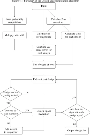
To explore this design space an algorithm (Appendix D) is proposed. The algorithm computes the average error of each of the designs and estimates the cost. The cost and error of each of the designs are compared and the optimal designs are chosen. A flowchart of the algorithm can be seen in Figure 4.1.

Input

The algorithm has 3 inputs: Input data for a MAC in the wanted distribution, the error magnitudes and cost estimations for each of the2×2bit multipliers.

Error probability computation

Using the input data the probability of an error occurring is calculated. The algorithm only includesM2, M3andM4of the aforementioned multipliers which means the probability of an error occurring in the 2×2bit multiplier is always equal to the probability the inputs of that multiplier are both3. The probability of each of the inputs being3is computed with equation (4.1). The probability the input for the given2×2bit multiplier is3is the amount of times it was3in the distribution sample (MA=3) divided by the total amount

of generated numbers (Mtotal). Then to get the probability of an error occurring for each multiplier the correct input probabilities are multiplied as shown in equation (4.2). This is done for each of the multipliers and a vector containing the 16 values for the error probability is output to the next step.

P(A= 3) = MA=3 Mtotal

(16)

[image:16.595.125.474.176.702.2]

Figure 4.1: Flowchart of the Design Space Exploration algorithm

Input

Error probability computation

Multiply with shift Calculate Er-ror magnitude

Calculate Av-erage Error for

each design

Sort designs by cost

Calculate Per-mutations

Calculate Cost for each design

Pick out best design

Design has best quality so far?

Does the de-sign overflow?

Add design to output list

Design Space Reduction

Are there de-signs left in the

design space?

Output design list no

yes

no

yes

(17)

[image:17.595.90.544.120.336.2]

Table 4.1: Example of a few sets of permutations

design 1 2 3 4 5 6 7 8 9 10 11 12 13 14 15 16

X1 M2 M2 M2 M2 M3 M4 M2 M2 M3 M2 M2 M2 M3 M2 M3 M2

X2 M2 M2 M2 M2 M3 M4 M2 M2 M3 M2 M2 M2 M3 M2 M3 M3

.. .. .. .. .. .. .. .. .. .. .. .. .. .. .. .. ..

Table 4.2: Example of a few sets of error magnitudes

design 1 2 3 4 5 6 7 8 9 10 11 12 13 14 15 16

X1 -2 -2 -2 -2 +2 -4 -2 -2 +2 -2 -2 -2 +2 -2 +2 -2

X2 -2 -2 -2 -2 +2 -4 -2 -2 +2 -2 -2 -2 +2 -2 +2 +2

.. .. .. .. .. .. .. .. .. .. .. .. .. .. .. .. ..

P(A= 3andB= 3) = MA=3∗MB=3 M2

total

(4.2)

Multiply with shift

The 16 probability values are multiplied with the needed shift for the outputs of the2×2multipliers shown in equation (1.2).The shifted probability values,Si∗P(E)iin equation (2.1), are the output.

Calculate Permutations

The number of different2×2 bit multipliers is used to generate all different design permutations. In the current configuration it calculates for 3 different multipliers. They are permutations with repetition which results as mentioned in316 = 43046721different designs. This block outputs 43 million sets of 16 numbers representing each multiplier in each design. Table 4.1 shows an example of a few of those 43 million sets. Here isX1the index of the designs and the numbers in the top row represent the sixteen2×2 multiplier locations in the MAC.

Calculate Error magnitude

The numbers representing the multipliers are replaced with the error magnitude of each of the multipliers resulting in 43 million sets of 16 error magnitudes. Table 4.2 shows an example of a few of those 43 million sets.

Calculate Average Error for each design

Each set of 16 error magnitudes is multiplied with the shifted probability (Si∗P(E)i) to get the average error each of the multipliers contributes to the whole8×8bit multiplier. These are then added up to get the average error of the whole multiplier. The output is a vector with an average error for each of the designs.

Calculate Cost for each design

The generated numbers representing all design permutations are replaced with the estimations for cost. These costs are added up to get an estimated cost for each of the 43 million designs.

Sort designs by cost

(18)

Pick out best design

From the sorted lists the designs with both the lowest cost and best quality (lowest average error) are taken and output to be used in the next steps.

Design has best quality so far?

In this block a check is done if the chosen optimal designs have the best quality so far. The algorithm checks the design space in order, from lowest to the highest cost. If the new design has a lower quality it means that both the cost is higher and the quality worse than it’s predecessors and it can be removed from the design space.

Does the design overflow?

As discussed in chapter 3, theM3multiplier makes positive errors which can cause the output to exceed 16 bits. This can also happen with the designs containing someM3multipliers. This is not wanted and these designs will be removed from the design space. Normally the overflow can be checked by calculating 255∗255for this is the largest number and will contain all the positive errors. However becauseM4has such a large error, the biggest number is actually2∗3 = 6instead of3∗3 = 5. This means there is a chance the multiplier will not overflow calculating255∗255but will overflow calculating a lower sum. This makes checking for overflow a lot more complicated. It can be checked by just checking all possible 8×8multiplications. However when this has to be done for a lot of designs it will take a lot of time. To speed up the algorithm, a few logic steps are done first, specific to the multipliers used in this work. For example the4×4bit multiplications will never overflow if the most significant multiplier is not theM3 multiplier. The other logic steps can be seen in the algorithm in appendix D. The last few designs that did not get filtered out using these logic steps are tested by calculating all possibilities.

Add design to output list

When the designs do not overflow and have the best quality so far they are added to the output list of the algorithm.

Design Space Reduction

If the design overflows, that specific design will be removed from the design space. Otherwise all designs with the same cost as that design will be removed from the design space.

Are there designs left in the design space?

(19)

Chapter 5 Results

In this chapter the design space exploration algorithm is run and the results are discussed. Then a few reccomendations for future work are made.

5.1 Results of design space exploration

The algorithm discussed in the last chapter was used to find the optimal designs using the2×2bit elements M2,M3andM4. The corresponding error magnitudes are−2,+2and−4respectively. The estimations of the costs are based on the values in Table 3.2 in chapter 3. The values are 136₁₆ = 8.5,170₁₆ = 10.6and

136

16 = 8.5. Here the value for theM3multiplier differs from the one gained in the cost chapter because

the 17th bit is not taken into account. The algorithm removes designs with overflow so this will not be a problem. The algorithm was run for the uniform distribution, a normal distribution whereσ = 40and a normal distribution withσ= 50. The results are shown in Figure 5.1. The left side shows the total explored design space and the right side a zoomed version that is focused on the part with the lowest average errors. The black dots represent the43∗106designs and their calculated average errors and cost estimations. The red dots represent the designs removed by the overflow handling of the algorithm. Finally, the blue line connects the chosen designs with optimal average error for each cost.

The resulting optimal designs were checked with the methods discussed in chapter 3. The results can be found in Figure 5.2.

(20)

135 140 145 150 155 160 165 170 Estimated Cost 0 200 400 600 800 1000 1200 1400 1600 1800 2000 A verage Error

140 142 144 146 148 150 152 154 156

Estimated Cost 0 0.02 0.04 0.06 0.08 0.1 0.12 0.14 A verage Error

(a) Uniform Distribution (left: Total design space, right: Zoomed version at low average errors)

135 140 145 150 155 160 165 170 Estimated Cost 0 50 100 150 200 250 300 350 A verage Error

142 144 146 148 150 152 154 156 158 160 Estimated Cost 0 0.002 0.004 0.006 0.008 0.01 0.012 0.014 A verage Error

(b) Normal Distributionσ= 40(left: Total design space, right: Zoomed version at low average errors)

135 140 145 150 155 160 165 170 Estimated Cost 0 100 200 300 400 500 600 A verage Error

144 146 148 150 152 154 156 158 160 Estimated Cost 0 0.005 0.01 0.015 0.02 0.025 0.03 A verage Error

[image:20.595.94.513.144.303.2]

(c) Normal Distributionσ= 50(left: Total design space, right: Zoomed version at low average errors)

(21)

136 138 140 142 144 146 148 150 152 Area [LE]

0 1 2 3 4 5 6

MPE

[%]

(a) Uniform Distribution

135 140 145 150 155 160

Area [LE] 0

0.1 0.2 0.3 0.4 0.5 0.6 0.7 0.8 0.9 1

MPE [%]

136 138 140 142 144 146 148 150

Area [LE]

0 0.2 0.4 0.6 0.8 1 1.2 1.4 1.6 1.8

MPE [%]

[image:21.595.204.398.146.682.2]

(22)

[image:22.595.153.450.118.761.2]

Table 5.1: Found Designs (a) Uniform Distribution

designs D1 D2 D3 D4 D5 D6 D7 D8 D9

AHHBHH M2 M3 M3 M3 M3 M3 M3 M3 M3

AHLBHH M2 M2 M2 M2 M2 M4 M4 M4 M4

AHHBHL M2 M4 M4 M4 M4 M4 M4 M4 M4

AHLBHL M2 M2 M3 M2 M2 M3 M3 M3 M3

AHHBLH M2 M2 M2 M2 M2 M2 M2 M2 M3

AHHBLL M2 M2 M4 M2 M2 M2 M2 M3 M2

AHLBLH M2 M2 M2 M3 M3 M2 M2 M4 M4

AHLBLL M2 M2 M2 M2 M4 M2 M4 M3 M4

ALHBHH M2 M2 M4 M2 M2 M3 M3 M3 M2

ALHBHL M2 M2 M4 M4 M4 M4 M4 M4 M4

ALLBHH M2 M2 M4 M2 M2 M3 M3 M2 M3

ALLBHL M2 M4 M2 M2 M4 M2 M4 M2 M3

ALHBLH M2 M4 M2 M2 M3 M2 M3 M3 M3

ALHBLL M2 M2 M4 M2 M4 M4 M4 M4 M3

ALLBLH M2 M2 M4 M2 M4 M4 M4 M4 M2

ALLBLL M2 M2 M2 M3 M3 M3 M3 M3 M3

designs D1 D2 D3 D4 D5 D6 D7 D8 D9

AHHBHH M2 M2 M2 M2 M2 M4 M2 M2 M2

AHLBHH M2 M2 M2 M3 M3 M3 M2 M3 M3

AHHBHL M2 M2 M3 M3 M3 M3 M3 M4 M4

AHLBHL M2 M3 M3 M3 M3 M3 M3 M2 M3

AHHBLH M2 M2 M2 M2 M2 M2 M3 M3 M3

AHHBLL M2 M2 M2 M4 M4 M2 M3 M2 M2

AHLBLH M2 M2 M2 M4 M4 M3 M2 M3 M3

AHLBLL M2 M2 M2 M2 M4 M4 M3 M4 M4

ALHBHH M2 M2 M2 M2 M2 M4 M3 M3 M3

ALHBHL M2 M2 M2 M4 M4 M2 M2 M3 M3

ALLBHH M2 M2 M2 M4 M4 M2 M4 M2 M4

ALLBHL M2 M2 M2 M4 M4 M4 M2 M3 M3

ALHBLH M2 M2 M2 M2 M2 M4 M2 M2 M4

ALHBLL M2 M2 M2 M4 M2 M2 M2 M2 M3

ALLBLH M2 M2 M2 M4 M3 M4 M2 M2 M3

ALLBLL M2 M2 M2 M4 M4 M3 M2 M2 M3

designs D1 D2 D3 D4 D5 D6

AHHBHH M2 M3 M2 M2 M2 M2

AHLBHH M2 M4 M3 M3 M3 M3

AHHBHL M2 M2 M3 M3 M3 M3

AHLBHL M2 M2 M2 M3 M3 M3

AHHBLH M2 M2 M2 M2 M2 M4

AHHBLL M2 M2 M2 M2 M2 M2

AHLBLH M2 M2 M2 M2 M2 M3

AHLBLL M2 M2 M2 M2 M2 M2

ALHBHH M2 M2 M2 M2 M4 M4

ALHBHL M2 M2 M2 M2 M3 M3

ALLBHH M2 M4 M2 M2 M2 M4

ALLBHL M2 M2 M2 M2 M2 M2

ALHBLH M2 M2 M2 M2 M4 M4

ALHBLL M2 M2 M2 M2 M2 M4

ALLBLH M2 M2 M2 M2 M4 M4

(23)

[image:23.595.155.449.230.641.2]

Table 5.2: Design results (a) Uniform Distribution

designs Average Error

Estimated

Cost [LE] MSE MPE Cost [LE]

D1 9.03∗102 136 8.16∗1013 5.55% 136

D2 1.12∗101 _138.1 ₅_.₃₅_∗₁₀10 ₀_._11% ₁₃₇ D3 1.30∗10−1 140.2 3.80∗1010 0.10% 140

D4 8.62∗10−2 142.3 3.79∗1010 0.09% 145

D5 8.52∗10−2

144.4 3.79∗1010 ₀_._10%

143

D6 6.63∗10−2 146.5 4.07∗1010 0.10% 150

D7 6.52∗10−2

148.6 4.08∗1010 ₀_._10%

151

D8 6.42∗10−2 150.7 4.09∗1010 0.10% 150

D9 6.34∗10−2 _152.8 ₄_.₀₈_∗₁₀10 ₀_._10% ₁₅₃

Estimated

D1 1.55∗102

136 2.41∗1012 ₀_._95%

136

D2 9.12∗101 138.1 8.34∗1011 0.56% 139

D3 3.43∗101

140.2 1.21∗1011 ₀_._21%

140

D4 1.33∗10−2 142.3 3.41∗109 0.03% 143

D5 1.31∗10−2 _144.4 ₃_.₄₀_∗₁₀9 ₀_._03% ₁₄₈ D6 2.15∗10−3 146.5 1.00∗1010 0.05% 148

D7 1.70∗10−3 148.6 3.29∗109 0.03% 150

D8 4.56∗10−5

152.8 5.43∗109 ₀_._04%

158

D9 7.60∗10−6 157.0 5.42∗109 0.04% 160

Estimated

D1 2.63∗102 ₁₃₆ ₆_.₉₄_∗₁₀12 ₁_._61% ₁₃₆ D2 1.61∗102 138.1 2.59∗1012 0.98% 137

D3 6.44∗101 140.2 4.24∗1011 0.39% 142

D4 8.18∗10−1

142.3 8.55∗109 ₀_._05%

143

D5 2.52∗10−2 144.4 8.77∗109 0.05% 145

D6 2.25∗10−3

146.5 9.12∗109 ₀_._05%

(24)

5.2 Conclusion and discussion

The goal of this work is to find an approximate design of an 8 bit MAC which has the lowest cost for a given quality or the best accuracy for a given cost. The algorithm achieves this and outputs the optimal designs for each cost. Compared to conventional multipliers likeM1andM2, the designs found by the algorithm have a much lower error for a small increase in cost and the overall quality-cost tradeoff is improved. For example, the uniform distribution has a value ofM P Ethat is5.44%lower for an increase of only 1 logic element in area (D2in Table 5.2(a)) over the multiplier made with2×2bit elementM2(Table 3.1 and Table 3.2).

When taking a closer look at the results and comparing the results from the algorithm with the result of the Quality and Cost Analysis tests, the algorithm seems to come reasonably close with its estimations. When looking at the zoomed version of the normal distribution withσ= 50in Figure 5.1(c) the line connecting the chosen optimal designs suddenly stops. This means the algorithm did not find any designs with lower average error at a higher cost.

The values of MPE and MSE in Table 5.2 are mostly in descending order since the designs are sorted on the calculated average error of the algorithm. There are a few values that stand out however, for they are not in order like the rest. For exampleD4of the uniform designs has the lowest error according to the Quality Analysis while not at the lowest spot. In the same wayD6from the normal distribution withσ= 40has a higher error. The error is really small however and these differences are most likely the result of estimation in the algorithm. Also the inputs used to test the quality are random and therefore the errors not always perfectly cancel eachother.

When comparing the estimated and actual cost of the designs the values seem to come close. However a important part of the goal is that the actual cost should be in ascending order like the estimated costs. When looking atD5andD8of the uniform distribution it can be seen that this is not always the case. They have a lower cost than the designsD4andD7respectively and are therefore (theoretically) objectively better designs as they have a lower error and lower cost. This indicates that the area is not only dependent on the used multipliers and that the estimation based on this assumption is not accurate enough. The difference in cost is most likely caused by the fact thatM2andM4only output 3 bits instead of 4. This can change the size of the adders needed within each4×4bit multiplier segment depending on the location ofM2orM4. This makes the total area of the MAC differ between two multiplier designs using the same multipliers but in a different configuration. The algorithm is reasonably fast and completes a single run in a few minutes. When the algorithm is adjusted to take into account 4 instead of 3 different multipliers the needed memory to run the algorithm increases exponentially. This is the result of the algorithm calculating the quality and cost for every permutation of which there are416 _{= 4}_.₃_{billion for 4 multipliers instead of the 43 million}

(25)

5.3 Future work

• As discussed in theDiscussion, the cost estimation is inaccurate. The effect of the configuration of the multipliers on the area should be investigated and the results can be implemented in the estimation of the cost. The algorithm should then be able to more accurately find the optimal designs.

• The cost estimation of the algorithm can also be rewritten to express something completely different, for example the energy consumption of the multiplier. These different properties of the multiplier can also be combined to form an abstract cost value to find optimal designs.

• The algorithm only works with2×2bit multiplier elements creating an error when calculating3×3. This can be changed to add in, for example, multiplierM1by rewriting the probability calculation and error magnitude parts of the algorithm.

(26)

Bibliography

[1] Larry R. D0Addario and Douglas Wang. An integrated circuit for radio astronomy correlators support-ing large arrays of antennas.Journal of Astronomical Instrumentation, 05(02):1650002, 2016.

[2] M. Shafique, R. Hafiz, S. Rehman, W. El-Harouni, and J. Henkel. Invited: Cross-layer approximate computing: From logic to architectures. In2016 53nd ACM/EDAC/IEEE Design Automation Confer-ence (DAC), pages 1–6, June 2016.

[3] Q. Xu, T. Mytkowicz, and N. S. Kim. Approximate computing: A survey.IEEE Design Test, 33(1):8– 22, Feb 2016.

[4] Semeen Rehman, Walaa El-Harouni, Muhammad Shafique, Akash Kumar, and J¨org Henkel. Architectural-space exploration of approximate multipliers. In Frank Liu, editor,ICCAD, page 80. ACM, 2016.

[5] Parag Kulkarni, Puneet Gupta, and Milos D. Ercegovac. Trading accuracy for power with an underde-signed multiplier architecture. InVLSI Design, pages 346–351. IEEE Computer Society, 2011.

[6] S. S. Shalom and J. Tabrikian. Efficient computation of mse lower bounds via matching pursuit.IEEE Signal Processing Letters, 24(12):1798–1802, Dec 2017.

(27)

(28)

Appendix A

Matlab code to model a MAC and test

for quality

A.1 MAC Model

A.1.1 MacSpeed

function [ res ] = macSpeed(I1,I2,mul)

%This function first calculates the product using the FullMulSpeed function and %then adds the results.

res = sum(FullMulSpeed(I1,I2,mul),2);

end

A.1.2 FullMulSpeed

function [ r ] = FullMulSpeed( I1, I2, mul )

%FULLMULSPEED Matlab model of a 8x8 bit Multiplier. I1 and I2 are the input vectors and %mul is a 16 element vector describing which 2x2 bit multiplier to use in

%which location. The 2x2 bit multipliers are defined in TwoBitMulSpeed

d1 = I1; d2 = I2;

a1 = mod(d1,4); %mod will give the leftovers of the input divided by 4 which ranges from

0 - 3

a2 = mod(d2,4); %this is the least significant 2 bits of the input.

d1 = d1 - a1; %the leftovers are substracted from the inputs

d2 = d2 - a2;

b1 = mod(d1,16); %this gives the next 2 bits of the input

b2 = mod(d2,16); d1 = d1 - b1; d2 = d2 - b2; c1 = mod(d1,64); c2 = mod(d2,64);

d1 = (d1 - c1)/64; %The output is divided by the shift of the multiplier

d2 = (d2 - c2)/64; %this is to get all the 2bit inputs in a range of 0-3

(29)

x1 = TwoBitMulSpeed(a1,a2,mul(1)); %the 16 multiplications are done using TwoBitMulSpeed

x2 = TwoBitMulSpeed(a1,b2,mul(2)).*4; %the input mul(x) defines the correct 2x2 bit

multiplier used

x3 = TwoBitMulSpeed(b1,a2,mul(3)).*4; %The output is multiplied with the needed shift.

x4 = TwoBitMulSpeed(b1,b2,mul(4)).*16; x5 = TwoBitMulSpeed(a1,c2,mul(5)).*16; x6 = TwoBitMulSpeed(a1,d2,mul(6)).*64; x7 = TwoBitMulSpeed(b1,c2,mul(7)).*64; x8 = TwoBitMulSpeed(b1,d2,mul(8)).*256;

x9 = TwoBitMulSpeed(c1,a2,mul(9)).*16;

x10 = TwoBitMulSpeed(c1,b2,mul(10)).*64; x11 = TwoBitMulSpeed(d1,a2,mul(11)).*64; x12 = TwoBitMulSpeed(d1,b2,mul(12)).*256; x13 = TwoBitMulSpeed(c1,c2,mul(13)).*256; x14 = TwoBitMulSpeed(c1,d2,mul(14)).*1024; x15 = TwoBitMulSpeed(d1,c2,mul(15)).*1024; x16 = TwoBitMulSpeed(d1,d2,mul(16)).*4096;

r = x1 + x2 + x3 + x4 + x5 + x6 + x7 + x8 + x9 + x10 + x11 + x12 + x13 + x14 + x15 + x16

; % the outputs of all multiplications are added together to get the total output.

end

A.1.3 TwoBitMulSpeed

function [ r ] = TwoBitMulSpeed( I1, I2, mul )

%TWOBITMULSPEED This function calculates I1 * I2 and then changes the %output to match the error made by the approximate 2x2 multiplier defined %in mul.

switch(mul)

case 1 %accurate

r = I1.*I2;

case 2 %M1

r = I1.*I2; %calculate the exact result of 2x2 multiplier

r(r==3) = 2; %add the errors in

r(r==1) = 0;

case 3 %M2

r = I1.*I2; r(r==9) = 7;

case 4 %M3

r = I1.*I2; r(r==9) = 11;

case 5 %M4

r = I1.*I2; r(r==9) = 5;

end

A.2 Quality test

A.2.1 QualityCheck

function [ Q ] = QualityCheck( I1,I2,di )

%QUALITYCHECK This function calculates both the MPE and MSE for given input

%samples I1 and I2. di is a matrix containing a list of designs with 16 values for 2x2 multipliers for each design.

(30)

h = waitbar(0,'Calculating Quality'); %progress bar

Accdot = dot(I1,I2,2); %calculating accurate dot product.

for i=1:size(di,1) %for each design in the list di

waitbar(i/size(di,1),h); %update progress bar

mul = di(i,:); %select ith design in the list

Macdot = macSpeed(I1,I2,mul); %perform inaccurate mac operation

mpe = [mpe; MPE(Accdot,Macdot)]; %calculate MPE

mse = [mse; MSE(Accdot,Macdot)]; %calculate MSE

end

Q = [mse mpe]; %output list

delete(h) clearvars h

end

A.2.2 MSE

function [ Error ] = MSE( Acc, Ax )

%MSE This function calculates the Mean Square Error. Acc are the accurate MAC %results and Ax the approximate results.

Error = sum((Acc-Ax).ˆ2)/size(Acc,1);

end

A.2.3 MPE

function [ Error ] = MPE(Acc, Ax)

%MPE This function calculates the Mean Percentage Error. Acc are the accurate MAC %results and Ax the approximate results.

Error = 100*sum(abs(Acc-Ax)./Acc)/size(Acc,1);

(31)

Appendix B

VHDL code of the MAC

B.1 MAC

LIBRARY IEEE;

USE IEEE.std_logic_1164.ALL;

USE IEEE.numeric_std.ALL;

USE work.ALL;

entity AccMAC is

port( i1, i2: in unsigned(7 downto 0);

CLK: in std_logic;

result: out unsigned(22 downto 0)

);

end AccMAC;

architecture bhv of AccMAC is

COMPONENT eightbitmultiplier is

port( i1, i2: in std_logic_vector(7 downto 0);

result: out std_logic_vector(15 downto 0)

);

end COMPONENT;

signal mul: std_logic_vector(15 DOWNTO 0);

signal total, Rtotal: unsigned(22 downto 0) := (others => '0');

begin

--eight bit multiplier:

Mult: eightbitmultiplier PORT MAP(i1 => std_logic_vector(i1) , i2 =>

std_logic_vector(i2) , result => mul);

--sum up all inputs:

total <= Rtotal + resize(unsigned(mul), 23);

PROCESS(CLK)

BEGIN

IF rising_edge(CLK) THEN

Rtotal <= total; --next clock cycle update output

END IF;

END PROCESS; result <= Rtotal;

end architecture;

B.2 eightbitmultiplier

LIBRARY IEEE;

(32)

USE work.ALL;

entity eightbitmultiplier is

);

end eightbitmultiplier;

architecture eighttofour of eightbitmultiplier is COMPONENT fourbitmultiplier is

);

end COMPONENT;

signal temp1, temp2, temp3, temp4: std_logic_vector(7 downto 0);

begin

mul1: fourbitmultiplier PORT MAP(i1 => i1(3 downto 0) , i2 => i2(3 downto 0) ,

result => temp1); --LSB

result => temp2); --MidSB

result => temp4); --MSB

result <= std_logic_vector(resize(unsigned(temp1), 16) + shift_left(resize( unsigned(temp2), 16),4) + shift_left(resize(unsigned(temp3), 16),4) +

shift_left(resize(unsigned(temp4), 16),8)); --shift the results and add up

end architecture;

B.3 fourbitmultiplier

LIBRARY IEEE;

USE work.ALL;

entity fourbitmultiplier is

);

end fourbitmultiplier;

architecture fourtotwo of fourbitmultiplier is COMPONENT twobitmultiplier is

);

end COMPONENT;

signal temp1, temp2, temp3, temp4: std_logic_vector(3 downto 0);

(33)

mul1: twobitmultiplier PORT MAP(i1 => i1(1 downto 0) , i2 => i2(1 downto 0) ,

result => temp1); --LSB

result => temp4); --MSB

result <= std_logic_vector(resize(unsigned(temp1), 8) + shift_left(resize( unsigned(temp2), 8),2) + shift_left(resize(unsigned(temp3), 8),2) +

shift_left(resize(unsigned(temp4), 8),4)); --shift the results and add up

end architecture;

B.4 Accurate twobitmultiplier

LIBRARY IEEE;

entity twobitmultiplier is

);

end twobitmultiplier;

architecture accurate of twobitmultiplier is signal temp: std_logic_vector(3 downto 0);

begin

temp(0) <= i1(0) and i2(1);

temp(1) <= i1(1) and i2(0);

temp(2) <= i1(1) and i2(1);

temp(3) <= temp(0) and temp(1);

result <= (temp(3) and temp(2)) & (temp(3) xor temp(2)) & (temp(0) xor temp(1))

& (i1(0) and i2(0)); --gate logic of the 2x2 multiplier

end architecture;

B.5 M1 twobitmultiplier

LIBRARY IEEE;

entity AM1twobitmultiplier is

);

end AM1twobitmultiplier;

architecture approx1 of AM1twobitmultiplier is signal temp: std_logic_vector(3 downto 0);

begin

temp(0) <= i1(0) and i2(1);

temp(1) <= i1(1) and i2(0);

temp(2) <= temp(0) and temp(1);

(34)

result <= temp(2) & (temp(2) xor temp(3)) & (temp(0) xor temp(1)) & temp(2); --gate logic of the 2x2 multiplier

end architecture;

B.6 M2 twobitmultiplier

LIBRARY IEEE;

);

begin

temp(0) <= i1(0) and i2(1);

temp(1) <= i1(1) and i2(0);

result <= '0' & (i1(1) and i2(1)) & (temp(0) or temp(1)) & (i1(0) and i2(0));

--gate logic of the 2x2 multiplier

end architecture;

B.7 M3 twobitmultiplier

LIBRARY IEEE;

);

begin

temp(0) <= i1(0) and i2(0);

temp(1) <= i1(0) and i2(1);

temp(2) <= i1(1) and i2(0);

temp(3) <= i1(1) and i2(1);

result <= (temp(3) and temp(0)) & (temp(3) and (not temp(0))) & (temp(1) or temp

(2)) & temp(0); --gate logic of the 2x2 multiplier

end architecture;

B.8 M4 twobitmultiplier

LIBRARY IEEE;

(35)

);

begin

temp(0) <= i1(0) and i2(1);

temp(1) <= i1(1) and i2(0);

result <= '0' & (i1(1) and i2(1)) & (temp(0) xor temp(1)) & (i1(0) and i2(0));

--gate logic of the 2x2 multiplier

(36)

Appendix C

RTL view of the MAC synthesised by

Quartus

C.1 MAC

eightbitmultiplier:Mult i1[7..0] i2[7..0] result[15..0] Rtotal[22..0] D CLK SCLR 23'h0 Q + Add0 CIN 1'h0 A[22..0] B[22..0] OUT[22..0] CLK i1[7..0] i2[7..0] result[22..0] 15:0

C.2 8 bit multiplier

i1[7..0] fourbitmultiplier:mul4 i1[3..0] i2[3..0] result[7..0] fourbitmultiplier:mul2 i1[3..0] i2[3..0] result[7..0] fourbitmultiplier:mul3 i1[3..0] i2[3..0] result[7..0] i2[7..0] result[15..0] + Add0 CIN 1'h0 A[8..0] B[8..0] OUT[8..0] ₊ Add1 CIN 1'h0 A[9..0] B[9..0] OUT[9..0] ₊ Add2 CIN 1'h0 A[7..0] B[7..0] OUT[7..0] fourbitmultiplier:mul1 i1[3..0] i2[3..0] result[7..0] 7:0 8:0 9:4 3:0 3:0 3:0 7:4 7:4 7:4 3:0 3:0 7:4 7:4 3:0 7:0 7:0

C.3 4 bit multiplier

(37)

Appendix D

Design space exploration Matlab

algorithm

D.1 FindDesign

function [de,Era,Ba,Co] = FindDesign( I1,I2, E, C)

%FINDDESIGN This function finds the optimal design for given input %distributions, error magnitudes and cost estimations.

%I1 and I2 are the input samples. E is the error magnitude of the 2x2 %multiplier and C is the estimation for cost for each multiplier. %outputs are: de - a list of the designs

% Era - the removed designs due to overflow

% Ba,Co - a list of all average errors and cost estimations

h = waitbar(0,'Calculating Weight and Chance of each multiplier'); %progress bar

W = FindWeight(I1,I2); %function for calculating weighted chance. (chance of error times

the shift of the multiplier location.

waitbar(0.115,h,'Loading permutations');

load('../Variables/Per.mat'); %loading the permutations variable.

waitbar(0.123,h,'Calculating Cost');

Co = sum(C(Per(1:20000000,:)),2); %Calculating cost estimations by summing up costs for

each design.

Co = [Co; sum(C(Per(20000001:end,:)),2)]; %Calculation divided in 2 for better memory

management (some memory troubles occured)

waitbar(0.246,h,'Calculating Balance');

Er = int8(E); %making sure the error magnitudes are in int8 format to prevent memory

overload.

Er = Er(Per); %inputing the errors into the permutations matrix

clearvars Per %clearing Per variable to clear up some memory

waitbar(0.38,h);

Ba = abs(double(Er)*W'); %calculating the average error for each design by multiplying

and adding up with the weighted chance.

de = []; Era = [];

c = unique(Co); %make a list of all different costs present

bd = 1000; %value of the current lowest average error, initialised at a high value

(1000)

waitbar(0.5,h,'Sorting and Overflow handling');

for i=1:size(c,1) %for each unique cost

waitbar((i/size(c,1))/2+.5,h);

(38)

b = Ba(a); %get the corresponding average errors of those designs

if min(b) < bd %if the lowest average error of those designs is lower then

the lowest average error so far

e = Er(a,:); %Make a list of the designs

end

while min (b) < bd %while the lowest average error of the list is still lower then the previous lowest

o = find(b == min(b)); %find the designs with the lowest average error

K = []; %empty list K - a list of designs that do not overflow

R = []; %empty list R - a list of designs that do overflow

[K,R] = FindOverflowFast(e(o,:)); %fill lists K and R

if isempty(K) ==0 %if list K is not empty

e=e(o,:); %get a list of the designs

de = [de;double(e(K,:)) ones(size(K,1),1)*c(i) ones(size(K,1),1)*min(b)]; %

add the designs and their cost and average error to the output list

bd=min(b); %update new lowest average error

else

b(o) = []; %remove designs from the list.

e(o,:)= [];

end

if isempty(R) ==0 %if list R is not empty

Era = [Era;min(b) c(i)]; %add designs to the list of designs that overflow

end

end end

waitbar(1,h,'Done');

delete(h)

end

D.2 FindWeight

function [ W ] = FindWeight( I1,I2 )

%FINDWEIGHT This function finds the weighted chance of an error occuring %I1 and I2 are the input samples.

d1 = I1; d2 = I2;

a1 = mod(d1,4); %mod will give the leftovers of the input divided by 4 which ranges from

0 - 3

a2 = mod(d2,4); %this is the least significant 2 bits of the input.

d1 = d1 - a1; %the leftovers are substracted from the inputs

d2 = d2 - a2;

b1 = mod(d1,16); %this gives the next 2 bits of the input

b2 = mod(d2,16); d1 = d1 - b1; d2 = d2 - b2; c1 = mod(d1,64); c2 = mod(d2,64);

d1 = (d1 - c1)/64; %The output is divided by the shift of the multiplier

d2 = (d2 - c2)/64; %this is to get all the 2bit inputs in a range of 0-3

c1 = c1/16; c2 = c2/16; b1 = b1/4; b2 = b2/4;

A = (size(a1(a1==3),1)/(size(a1,1)*size(a1,2)) + size(a2(a2==3),1)/(size(a2,1)*size(a2

,2)))/2; %for each 2bit part of the 8bit input the chance is calculated that it is

(39)

B = (size(b1(b1==3),1)/(size(b1,1)*size(b1,2)) + size(b2(b2==3),1)/(size(b2,1)*size(b2 ,2)))/2;

C = (size(c1(c1==3),1)/(size(c1,1)*size(c1,2)) + size(c2(c2==3),1)/(size(c2,1)*size(c2

,2)))/2;

D = (size(d1(d1==3),1)/(size(d1,1)*size(d1,2)) + size(d2(d2==3),1)/(size(d2,1)*size(d2

,2)))/2;

S=[1 4 4 16 16 64 64 256 16 64 64 256 256 1024 1024 4096]; %a list of the shifts needed

W= S.*[Aˆ2 A*B A*B Bˆ2 A*C A*D B*C B*D A*C B*C A*D B*D Cˆ2 C*D C*D Dˆ2]; %the

shifts are multiplied with the chance an error occurs(3*3 happens). end

D.3 FindOverflowFast

function [ O, E ] = FindOverFlowFast( D )

%FINDOVERFLOW This function uses some logic steps to speed up the overflow %check. This only works with the multipliers with error -2 +2 and -4 !!

% D are the designs that need to be checked O is the list that does not

% overflow and E the ist of designs that does.

O = []; E = [];

for i=1:size(D,1) %for all designs in list D

o=0; %start with the assumption the design does not overflow

for j=1:4 %for each set of 4 multipliers

if D(i,4*j)==2 %check if the most significant is M3 (3*3=11)

if nnz(D(i,(4*(j-1)+1):(4*j))==2)>2 %check if there are more then 2 M3 in

the set of 4

if (D(i,4*(j-1)+2) + D(i,4*(j-1)+2)) > (-2) %check if sum of specific

locations is higher then -2

o=1; %if all these statements are true the individual 4x4

multiplier does overflow.

end %otherwise the 4x4 multiplier does not overflow

end end end

%It is possible that no individual 4x4 multipliers overflow but the 8x8 %does. The following code deals with that

if o==0 %if the 4x4 already overflows there is no need to check

if D(i,16) == 2 %if the most significant 2x2 multiplier is M3 (3*3=11)

if nnz([D(i,12:15) D(i,8)] == -4) == 0 %if there are no M4 multipliers

present the design overflows.

o=1;

else

o=FindOverflowSlow(D(i,:)); %if there are the rest is checked with an

exhaustive check end

end end

if o==0 %if it does not overflow

O = [O;i]; %add it to the list

else

E = [E;i]; %else add it to the overflowing list

end end end

D.4 FindOverflowslow

function [ o ] = FindOverflowSlow(D)

%FINDOVERFLOWSLOW this function does an exhaustive search on a design to see if it overflows

%D is the design to check, o is 1 if it overflows and 0 otherwise

(40)

a(a==-4)=5; %change the designs indication from error magnitude (as worked with in FindDesign)

a(a==2)=4; %to a number (as worked with in the MAC model)

a(a==-2)=3;

k = [0:1:255]; %creating a matrix with all inputs

o = ones(1,256); i1 = k;

i2 = zeros(1,256);

for i = [1:255]

i1 = [i1 k]; i2 = [i2 i*o];

end

R = FullMulSpeed(i1,i2,a); %calculate all outputs with all inputs using the design D

o=0; %assume design does not overflow

if max(R)> 65535 %change it to overflow if the output exceeds 65535 (16 bits)

o=1;

end

Approximate multipliers for MAC

Approximate multipliers for MAC

Verstoep, B. (s1009966)

Contents

Introduction

MUL

+

Chapter 1

Approximate multipliers

1.1

Creating a multiplier

A

·B

A

·B

A

·B

A

·B

+

b

b

b

b

b

b

b

b

b

b

b

b

A:

{

A

A

{

{

b

b

b

b

B:

{

B

B

{

O

A

·B

A

·B

A

·B

A

·B

+

b

b

b

b

A:

{

A

A

{

b

b

b

b

{

A

A

{

b

b

b

b

{

B