Probability Analysis of Linear Time Logic
Statements on Infinite Walks in Large Random
Kripke Structures
Joran van den Bosse
1 July 2018
Abstract
Model checking is concerned to check the functionality of software and hardware systems. Those systems are discretised by labelled, directed graphs, which are called Kripke Structures. Due to the so-called state explosion problem those systems can become too large to be modelled by deterministic graphs This report uses the Erd¨os-R´enyi random graph model to model large systems. Linear Time Logic is used to describe events related to critical states in systems. Probabilities that basic Linear Time Logic statements hold, are computed. Former research showed that first order logic for graphs satisfied a zero-one law. In this paper it is investigated to what extent that result can be extended to Linear Time Logic statements on labelled, directed random graphs.
1
Introduction
When software or hardware systems are used, they are desired to satisfy cer-tain requirements. For instance, it is desirable that no states of the system can be reached that cause the system to crash. Model checking is a technique in computer science that checks whether software or hardware systems satisfy certain properties [1, page 330]. In this report we will be concerned with the probability that events related to critical states occur, such as their reachability.
According to [1, page 331] model checking often considers discrete models of such systems. One method to do this is to describe the system through so-called
Model checking statements are formulated using some specific logic. This pa-per focuses on statements that are formulated in Linear Time Logic, which is described on [1, page 334-336]. Linear Time Logic statements describe proper-ties of walks in Kripke Structures. For instance, the statement ”all vertices in the walk are healthy states” belongs to this logic. In the next section a formal definition of the logic is given. This paper focuses on the probability that all walks in a random graph starting from a fixed starting vertex satisfy a certain Linear Time Logic statement.
As is described on [1, page 343-344] hardware systems can have a lot of paral-lel components, causing a system to be able to reach a lot of different states. When such systems are modelled by directed graphs, the number of vertices can become large and it can be hard to describe such systems using deterministic graphs. This phenomenon is called thestate explosion problem.
These large systems can be modelled using Erd¨os-R´enyi random graphs [2]. In this model the number of vertices is a deterministic choice. However, the edges in the graph are selected at random using a given existence probability. This model was created by P. Erd¨os and A. R´enyi around 1960 [2] and has been applied to model networks. In this paper we use it to model the Kripke Struc-tures. In large systems there is a high number of states but the exact phase transitions are unknown. However, the density of phase transitions often can be determined. Therefore the random graph can be a good model to describe these systems.
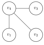
After P. Erd¨os and A. R´enyi had developed the random graph model a lot of re-search has been done on this field in order to extend the theory of deterministic graphs to the field of random graphs. For instance, in the theory of determin-istic graphs the term connectivity is used to describe graphs in which a path exists between any pair of vertices. An example of a connected graph is shown in figure 1. The question arose with what probability structural properties in graphs such as connectivity occurred in random graphs.
v4
v1 v2
[image:2.612.258.351.516.612.2]v3
Figure 1: A connected graph
the number of vertices of a graph grows infinitely large. Whether the probability tends to 0 or 1, depends on the edge existence probability. There exists some threshold value of the edge existence probability at which the structural prop-erty appears or disappears. For instance, in [2] it is shown thatp(n) =log(nn) is a threshold for connectivity. That is, if the edge existence probability is larger than this threshold and the number of vertices is large, it is almost surely con-nected and if the edge existence probability is lower, the graph is almost surely not connected. Since zero-one laws exist on a whole class of such properties, described by the so-called first order logic for graphs, it is possible that some class of Linear Time Logic statements also satisfies a zero-one law.
The aim of this probability analysis is to investigate whether such a zero-one law exists by computing the probability that basic Linear Time Logic statements hold. In section 2 formal definitions of the used structures are given. In section 3 an extension of former research on zero-one laws onto the model checking problem is considered. In section 4 a result on strong connectivity in directed random graph is presented. Then in sections 5 and 6 the probability analysis is executed. As a result of this analysis a further research on zero-one laws in model checking could become of interest.
2
Definitions
Before we start the probability analysis let us first consider some definitions. Let us firstly give a definition for the random graph model, as described by [5, page 2].
Definition 1 (Binomial Directed Random Graph). Let us consider a simple directed graph that containsnvertices and a real numberp, withp∈(0,1). For each of the n(n−1) ordered pairs of vertices let a directed edge exist between these vertices with probabilitypand no edge with probability 1−p. This graph is considered a Binomial Directed Random Graph. Such a graph is denoted by
G(n, p).
For the purpose of the model checking problem no loops are allowed in the graphs. After all in model checking only transitions between different states of a model are of interest. This is a slight difference to the model described by [5, page 2].
Definition 2 (Random Vertex Labelling). Let us consider a random graph
G(n, p). Choose a fixed real number q, with q∈(0,1). Each vertex of G(n, p)
receives a red label with probabilityqand a blue label with probability1−q.
Definition 3(Deterministic Vertex Labelling). Let us consider a random graph
G(n, p). Choose a fixed integer r, with r >0. If n≤r all vertices of G(n, p)
receive a red label. Ifn > rthe firstrvertices are labelled red and the remaining vertices receive a blue label.
The labelled, directed, binomial random graphs that are created using a combination of definition 1 and either definition 2 or 3 are the graphs considered in this paper. In order to apply model checking we consider walks through the graph, as described on [1, page 335].
Definition 4(Walk). Let us consider a directed graphG(V, E), whereV is the vertex set and E the edge set of the graph. A finite walk of length k through
G is a sequence of vertices of G, denoted as π =< π0, π1, ..., πk >, such that
for all i between 0 and k−1 the edge (πi, πi+1) is in edge set E. Here k is
a finite integer, with k > 0. An infinite walk is a sequence π=< π0, π1, ... >
such that for all positive i the edge (πi, πi+1) is in the edge set E. Vertex π0
is the starting vertex of the walk. The tail of the walk starting at vertexπj is
the sequence πj =< π
j, πj+1, ..., πk > in case of a finite walk or the sequence
πj=< π
j, πj+1, ... >in case of an infinite walk. The length of a walk, denoted
as|π|is the integer kif the walk is finite or ∞if it is an infinite walk.
Note that [1] uses the word ”path” instead of ”walk”. This paper stays in line with the choice of words in [6], since that is an elementary course on graph theory. In this paper only infinite walks will be considered and the first gen-erated vertex in a random graphG(n, p) will be the starting vertex of each walk.
A walk through a random graph models the running of a system that is con-sidered by model checking. Now the mathematical framework is given, let us consider the formal definitions of the discrete models of those systems. Those models are calledKripke Structure. We will consider the definition as given by [1, page 331-332].
Definition 5 (Kripke Structure). A Kripke Structure over a set of Atomic Propositions, denoted asAP, is a system described by the triple(S, R, I). Here
S is a set of states, R is a set of transition relations, with R ⊆ S×S, and
I is an interpretation of the atomic propositions belonging to the states. For each propositionp∈AP and for each state v∈S either p∈I(v) orp6∈I(v). ThereforeI is a function defined on the space I:S→2AP.
Definition 6 (Linear Time Logic). The Linear Time Logic in model checking defines whether a walkπin a Kripke Structure meets a statementφ, denoted as
π|=φ. A statement φin the language of Linear Time Logic is built using the following grammar rule:
φ:=p|¬φ|φ1∨φ2|X(φ)|F(φ)|G(φ)|U(φ, ψ)|W U(φ, ψ).
HereX(φ)is pronounced as Nextφ,F(φ)is pronounced as Finallyφ,G(φ)
is pronounced asGenerallyφ,U(φ, ψ)is pronounced asφUntilψandW U(φ, ψ)
is pronounced as φWeak Untilψ. These statements have the following logical interpretation:
π|=p ⇔ p∈I(π0)
π|=¬φ ⇔ π6|=φ
π|=φ1∨φ2 ⇔ π|=φ1∨π|=φ2
π|=X(φ) ⇔ π1|=φ
π|=F(φ) ⇔ ∃k∈ {k|0≤k <|π|}:πk |=φ π|=G(φ) ⇔ ∀k∈ {k|0≤k <|π|}:πk |=φ
π|=U(φ, ψ) ⇔ ∃k∈ {k|0≤k <|π|}: (i < k→πi|=φ)∧(πk |=ψ)
π|=W U(φ, ψ) ⇔ π|=U(φ, ψ)∨π|=G(φ).
Let us explain this definition with an example. Consider the graph in figure 2. Here some arbitrary Kripke Structure of six vertices is presented. The blue vertices are represented by circles and the red vertices by squares. Let v1 be the initial state of the system and let us consider the finite walk
π =< v1, v2, v4, v5, v2, v1 >. Since the initial state is blue, the statement
π|=blueis true. The next vertex in the walk,v2, is also a blue state. Conse-quently we haveπ|=X(blue). The fourth vertex in the walk,v5, is a red state. In this walk a red state is reached, soπ|=F(red). The walk contains both red and blue vertices. Consequentlyπ|=¬(G(red)∨G(blue)).
v6
v1 v2
v5
v3
[image:6.612.234.378.122.215.2]v4
Figure 2: A Kripke Structure of six states
3
Zero-One Law
Let us consider a binomial undirected random graph which is defined similarly as in Definition 1 with the difference that now edges are undirected. On [3, page 98-99] the definition of the First Order Logic for Graphs is given.
Definition 7 (First Order Logic for Graphs). A statement φ in the language of First Order Logic for Graphsmay contain the following elements: vertices, the equality sign (=) to state that two mentioned vertices are the same vertex in the graph, the adjacency sign (∼) to state that two vertices are adjacent, the logical connectives∧, ∨, ¬ and→ and the quantifiers ∀ and ∃. Here the =
and ∼ sign are assumed symmetric and∼is assumed antireflexive.
Independently [8] and [9] showed that statements formulated in First Or-der Logic for Graphs satisfy a zero-one law. That is, if the number of vertices goes to infinity the probability that such a statement is true goes to either 0 or 1.
Since that result applies for all statements in an entire logic the question arises whether the Linear Time Logic statements from model checking also satisfy such a zero-one law. If it were possible to write Linear Time Logic statements in the form of First Order Logic for Graphs a zero-one law would immediately have been proven to exist.
However, the Linear Time Logic statements causes problems when we try to rewrite statements into the First Order Logic for Graphs. Firstly, Linear Time Logic statements rely on the vertex labelling. The first order logic can only refer to vertices in general. In order to refer to vertices with certain properties, in this case the colours red and blue, sets have to be introduced. Allowing sets requires us to consider Second Order Logic, which does allow sets [7, page 143]. Then a set could be defined for each atomic proposition. For instance the statement
G(red) is true if every vertex that is reachable from the starting vertex, is in the set of red vertices. In first order logic such sets are not allowed.
isomorphism. Since there exist graphs that posses automorphisms this prevents us from defining Linear Time Logic statements as first order logic statements.
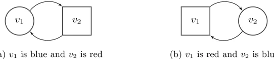
v1 v2
(a)v1 is blue andv2 is red
v1 v2
[image:7.612.172.443.162.221.2](b)v1 is red andv2is blue
Figure 3: Two graphs that have equal structure for first order logic
For instance, consider the graph of two vertices where there exists an edge in both directions and consider the starting vertex to be blue and the second vertex to be red, as displayed in figure 3a. Compare this to a similar graph where only the colour labels have changed (figure 3b). Let π be the infinite walk starting at initial statev1and then following the only outgoing edge from each state: π =< v1, v2, v1, v2, ... >. Since these two graphs are isomorphic, the statementπ|=redwould be either true or false for both graphs if it could be rewritten as a statement from the First Order Logic for Graphs. Since the statement is actually false in the first graph and true in the second graph, this is not a first order logic statement.
A second problem is that the random colouring makes it uncertain how many vertices will be red and how many will be blue. Logical statements have to be finite. The statement ”generally blue” is only true for a walk if no red vertex is reached. If it is uncertain how many red vertices exist, no finite statement can be made that states that no red vertices are reached. Likewise, the existence of a k-cycle, a cycle of k vertices, in an undirected random graph is a first order logic statement, while the existence of a cycle in general is not [3]. In order to apply logic on graphs to statements on walks we therefore are restricted to a deterministic colouring.
Thirdly, Kripke Structures are modelled by directed graphs instead of undi-rected graphs. In the definition of the First Order Logic for Graphs adjacency is assumed to be symmetric. However, in a directed graph symmetry is not a necessary condition for adjacency. If verticesv andware in a directed graph it is possible that the edge (v, w) exists while the edge (w, v) does not. It should be investigated whether the proofs of the theorems considering the zero-one laws in the First Order Logic for Graphs depend on the symmetry argument before they can be applied.
4
Strong Connectivity in Binomial Direct
Ran-dom Graphs
While the most results on random graphs consider undirected random graphs, [5] provides a useful result on directed random graphs. This result can be used in the probability analysis. After all, if in our case the graphs turn out to be almost surely strongly connected, all states are reachable from the initial state. In other words, reachability comes down to the analysis of components.
In [5] a threshold for strong connectivity is found. The following result states that a constant edge existence probability is greater than the given probability threshold. It is then quickly deduced that in this case graphs are almost surely strongly connected.
Theorem 1. Let G(n, p) be a Binomial Directed Random Graph and let the edge appearance probabilityp be constant. Then the probability that G(n, p) is strongly connected goes to 1 asn∞.
Proof. Let S be the property that a directed graph is strongly connected. Ac-cording to [5] bp = lnn+c
n is a threshold for strongly connectedness. That is,
strongly connectedness satisfies a zero-one law except if the chosen probabil-ity p is the same order as ˆp. In [5] it is shown that if for some random graph G(n, p) we have that p >> pˆ, which holds if limn→∞p
b
p > ∞, then
limn→∞P(G(n, p)∈ S) = 1. Now, letpbe constant. In that case we have:
lim
n→∞
p
b
p= limn→∞
pn
lnn+c
= lim
n→∞
p
1
n
= lim
n→∞pn =∞.
So when p is constant then we have that p >> pˆ. Therefore a directed random graph with constantpis strongly connected with probability 1 forn→ ∞.
In the following sections cover computations on basic Linear Time Logic Statements in random graphs with fixed edge probabilityp. Firstly we consider the Random Vertex Colouring of Definiton 2, secondly we consider the Deter-ministic Vertex Colouring of Definition 3. In those computations this result can be applied.
5
Random Colouring
assumed to have a random vertex colouring. The first generated vertex by random graphG(n, p) is considered to be the starting vertex and is denoted by
v1. Since we now focus on properties of all walks starting at the same initial state we use the following notation:
v|=φ ⇔ ∀π s.t. π0=v:π|=φ.
Here vis any state in the Kripke Structure andπis an infinite walk. Since we denote our initial state asv1, that state will be plugged into the statement above.
5.1
Generally Red and Generally Blue
Firstly consider the functions G(red) and G(blue). The probabilities that are computed areP(v1|=G(red)) andP(v1|=G(blue)). To compute the probability that these events occur let us use Theorem 1 thatG(n, p) is almost surely, that is with probability 1, strongly connected if n → ∞. In a strongly connected graph each vertex can be reached from the starting vertex. Therefore the events
v1|=G(red) andv1 |=G(blue) are only true if respectively all vertices are red or all vertices are blue. As a result we have the following results:
P(v1|=G(red)) =qn P(v1|=G(blue)) = (1−q)n.
Since we let the number of vertices grow infinitely large these probabilities vanish: P(v1|=G(red))→0 andP(v!|=G(blue))→0 asn→ ∞.
5.2
Finally Red and Finally Blue
Secondly let us compute the probabilities that the event ”finally red” or ”finally blue” occurs on each walk starting atv1. By definition the eventv1|=F(red) is true if for all walks starting atv1there exists ak≥0 such thatπk|=red. The first step of the computation ofP(v1|=F(red) is conditioning on the colour of
v1. After all, ifv1 is red the event π0|=redis true and thus we have found a nonnegative k such that πk |=red and such that for all i with 0 ≤ i < k we
have thatπi|=blue. The second condition is a result from the fact that
{i|0≤i <0, i∈Z}=∅.
This can be demonstrated using the Kripke Structure in figure 2 from section 2. There a blue cycle exists containing v1, the initial vertex, andv2. This allows the existence of walkπ=< v1, v2, v1, v2, ... >, which is a cycle that only contains blue vertices. Consequently,π6|=F(red) and thereforev16|=F(red). However, if edge (v2, v1) did not exist, each infinite walk would inevitably reach vertex
v5, which is coloured red. Then all walks starting atv1would meet F(red).
The aim now is to show thatv1 is almost surely part of some blue cycle and therefore the event v1 |= F(red) almost surely is false given that v1 is blue. The probability that there exists an outgoing edge fromv1 to any other edge equals p by definition of G(n, p). Similarly, an incoming edge to v1 from an arbitrary vertex exists with probabilityp. Thus the probability that both an outgoing and incoming edge exists to the same vertex equalsp2. Moreover the probability that any vertex is blue equals 1−q. Therefore the probability of both an outgoing and incoming edge occurring fromv1 to any other arbitrary vertex and that the other vertex is blue, equals p2(1−q). Let us define the random variableBn as the total number of blue vertices with both an outgoing
and incoming edge fromv1. Let us define the indicator random variablesIj as
follows:
Ij=
(
1 if edges (v1, vj) and (vj, v1) exist and vj is blue
0 else
We have shown in the previous paragraph that
Ij∼Bernoulli(p2(1−q)).
Now consider our definition ofBn:
Bn= n
X
j=2
Ij.
Since the distribution of the indicators is independent ofj, we have that
Bn∼Bin(n−1, p2(1−q)).
We can now deduce that P(Bn = 0) = (1−p2(1−q))n−1. Since p and q
are fixed probabilities strictly between 0 and 1 the number (1−p2(1−q) is also strictly between 0 and 1. As a resultP(Bn = 0)→0 asn→ ∞. In other words,
Now consider the required probability that the statement ”finally red” is true can be deduced using conditioning on the colour ofv1:
lim
n→∞P(v1|=F(red)) = limn→∞(P(v1|=F(red)|v1|=red)P(v1|=red) +P(v1|=F(red)|v1|=blue)P(v1|=blue)) = 1·q+ 0·(1−q)
=q.
In short, the probability that the statement ”finally red” is true for all walks starting atv1, equalsq. Similarly it can be deduced that ”finally blue” is true for all walks starting atv1 with probability 1−q.
Note that the stochastic element of model checking only appears in the cre-ation of the graph, not in the selection of walks. Intuitively one could expect these probabilities to be equal to 1. If we consider the graph to be a Markov chain and we would like to know whether an arbitrary walk would finally reach a red vertex, then we would indeed end up with probability 1. However, we are interested in the probability that every walk reaches a red vertex finally. This difference is similar to the use of a software package. Let a robot take arbitrary decisions. Then the system will almost surely end up in a critical state. How-ever, a human user could understand the package and know how to avoid the system to collapse, which resembles a blue cycle. This causes the probability of interest to be lower than 1.
5.3
Next Red and Next Blue
The third set of statements to consider are ”next red” and ”next blue” By definition the eventv1|=X(red) is true if the eventπ1|=redis true for all walks starting atv1. To be certain that the second vertex of each walk starting atv1 is red, we have to consider the probability thatv1has no outgoing edges to blue vertices. The probability that an outgoing edge exists to any arbitrary vertex equalspand the probability that such a neighbour is blue equals 1−q. Therefore similarly to previous computation a random variableBn can be defined. Only
this time this time the random variable is the number of outgoing edges to blue vertices. Therefore we have that
Bn∼Bin(n−1, p(1−q)).
This yields the following result:
P(Bn= 0) = (1−p(1−q))n→0 as n→ ∞.
5.4
Red Until Blue and Blue Until Red
The next considered statements are v1 |=U(red, blue) andv1 |=U(blue, red). The statement ”red until blue” is true for all walks if there exists ak≥0 such thatπk |=blueand for alli such that 0≤i < kwe have thatπi|=red.
These statements appear to be similar to ”finally blue” and ”finally red”. In fact, those statements turn out to be equivalent.
Theorem 2. Consider a Kripke Structure with initial statev1. The statements
v1 |= F(red) is true if and only if the statement v1 |= U(blue, red) is true.
Similarly, the statementv1|=F(blue)is true if and only if the statement v1|=
U(red, blue)is true.
Proof. Let us prove the equivalence betweenF(red) andU(blue, red). The other equivalence is proved similarly.
Let us assume that v1 |= F(red). Consider an arbitrary infinite walk π with
π0 =v1. By definition some k exists such that vertex πk is red. Let us now
consider the following set:
R={k|πk |=red}.
Now let us consider the minimum of setR:
k∗= min
k∈Rk.
Then we have that πk∗ |=red and if 0 ≤i < k∗ we have that πi |=blue.
Therefore we have thatπ|=U(blue, red). Sinceπis an arbitrary walk starting atv1 we have thatv1|=U(blue, red).
Conversely, assume thatv1|=U(blue, red). Let us consider an arbitrary walkπ such thatπ0=v1. By definition there exists aksuch thatπk|=red. Therefore we also have thatπ|=F(red) and consequently we have thatv1|=F(red).
An immediate result of theorem 2 is thatP(v1|=U(red, blue))→1−qand likewise that P(v1 |= U(blue, red)) → q as n → ∞. These are the required results.
Note that in general the statements π |= F(φ) and π |= U(ψ, φ) are not equivalent. For instance, let us consider the Kripke Structure in figure 2. Let
π=< v1, v6, v5, v2, v1, v2, v1, v2, ... > and compare the statements π|=F(red) and π |= U(red, red). The first statement is true, because vertex v5 is red. However, the initial vertexv1 is blue. Thereforeπ6|=U(red, red) in this case.
5.5
Red Weak Until Blue and Blue Weak Until Red
Theorem 3. Let us consider a Kripke Structure and any arbitrary walk π. Then the statementsπ|=W U(red, blue)andπ|=W U(blue, red) are true.
Proof. Let us prove the theorem for the statement π |= W U(red, blue). The second statements follows similarly.
The statement is true for an arbitrary walkπif one of two options is true. The first option is that there exists ak≥0 such thatπk |=blue and for allisuch that 0≤i < k it holds that πi|=red. The second option is that for allk≥0 it holds thatπk |=red. The aim is to show that always one of the options is
true. Let us consider a walk for which the second option is false. Then there has to exist ak≥0 such that πk |=blue. Let us pick the smallestk such that
πk|=blue. Thiskcan be picked in the definition ofU(red, blue). Therefore the
first option is true.
Conversely, if the first option is false then nokcan be found such thatπk |=blue.
As a resultG(red) is true, which is our second option.
Since one of both statements has to be true, the statement W U(red, blue) is true for all walks.
By theorem 3 it is guaranteed that P(v1 |=W U(red, blue))→1 and simi-larlyP(v1|=W U(blue, red))→1 asn→ ∞.
These were all the basic functions of the Linear Time Logic. It can be seen that the probability that all walks satisfy a basic Linear Time Logic statement either satisfies a zero-one law or solely depends on the colour of the starting ver-tex. This partly confirms the conjecture that all Linear Time Logic Statements satisfy some zero-one law. In order to investigate this possibility further, let us consider some embedded statements.
5.6
Finally Generally Red and Finally Generally Blue
Firstly, consider the statementsF G(red) andF G(blue). All walks satisfy these statements if for all walks there exists an i ≥ 0 such that for all k ≥ i it respectively holds that πk |= red or πk |= blue. That means that each walk
reaches a point from which all vertices in the tail of the walk have the same colour. Since by Theorem 1 the graph is almost surely strongly connected ifn
is large, this can only be true if allnvertices have the same colour. All vertices are red with probabilityqn and all vertices are blue with probability (1−q)n.
Since those probabilities go to 0 asn→ ∞it holds thatP(v1|=F G(red))→0 andP(v1|=F G(blue))→0 asn→ ∞.
5.7
Generally Finally Red and Generally Finally Blue
Secondly consider the reverse embedding: GF(red) andGF(blue). These state-ments hold for all walks if for alli≥0 there exists ak≥isuch that respectively
πk |=redor πk |=blue. Let us focus onGF(red), as GF(blue) is shown
probability that v1 is not contained in any 2-cycle of blue vertices goes to 0. Since that proof was not restricted to any specific vertex as only general prop-erties of the graph were used, it can likewise be shown that the blue neighbour ofv1 is almost surely contained in some blue cycle. Therefore a walk exist of which the tail only contains blue vertices. As a resultP(v1 |= GF(red))→ 0 andP(v1|=GF(blue))→0 asn→ ∞.
5.8
Red Until Generally Finally Red
Finally, consider one larger embedded statement: U(red, GF(red). This state-ment is true if for all walks some k ≥ 0 exists such that for all i such that 0≤i < kit holds thatπi |=redand that for alla≥kthere exists ab≥asuch that πb |=red. One requirement of this long statement is that the tail of the walk cannot only contain blue vertices. As was shown previously the starting vertex almost surely has a blue neighbour that is contained in some 2-cycle with only blue vertices. ThereforeP(v1|=U(red, GF(red))→0 asn→ ∞.
As can be seen a if some arbitrary embedded statements are selected the prob-ability that all walks satisfy the statements either goes to 0 or 1. Therefore the possibility of a zero-one law on Linear Time Logic statements still exists.
6
Deterministic Colouring
Let us now focus on the deterministic vertex colouring. Again the aim is to compute the probability that all walks starting atv1 satisfy some basic Linear Time Logic statement. The difference with previous section is the colouring method. Since the number of red vertices is finite in this section, this fraction of red vertices will vanish. With the random colouring it is expected that a fractionq of all vertices are red, withq ∈(0,1). Here that fraction is nr, with
r. This goes to 0 asnbecomes infinitely large. This results in some differences compared to the random colouring.
6.1
Generally Red and Generally Blue
Let us again start with the functionsG(red) andG(blue). According to Theorem 1 the random graph is almost surely strongly connected if n becomes large. Based on Defenition 3 some integerris fixed such that the first r vertices are red and the remaining vertices are blue. When n → ∞ but r is fixed it is certain thatn > r. Therefore blue vertices will appear in the graph. Since the graph is strongly connected there will almost surely exist a walk containing a blue vertex. Consequentely,P(v1|=G(red))→0 andP(v1 |=G(blue))→0 as
6.2
Finally Red and Finally Blue
Secondly, consider the statements F(red) and F(blue). When the random colouring method was applied the probability that all walks satisfied one of these statements depended on the colour of the starting vertex. In this case by assumption the starting vertex is red. ThereforeP(v1|=F(red))→1 asn→ ∞.
On the other hand all walks meet F(blue) if all walks at some point have to reach a vertex other than the firstrvertices. The statement is therefore false if in the firstrvertices some red cycle exists that can be reached from the starting vertex. The probability that such a walk exists is equal to the probability that in the finite random graphG(r, p) a cycle exists that can be reached from vertexv1.
This probability is hard to compute. Therefore this probability will be denoted with the symbolP. Therefore we have P(v1|=F(blue))→1−P. However, it is possible to derive an upper and lower boundary for 1−P.
If v1 has no outgoing vertices to any other red vertex, it is certain that the second vertex in each walk is blue. Each edge appears independently with prob-abilityp. Therefore, the probability that no edge exists fromv1 to any other red vertex equals (1−p)r−1. This is a lower boundary for
P(v1|=F(blue)).
To determine an upper boundary, let us define Rr as the number of 2-cycles
containingv1 and only containing red vertices. Similarly to section 5.2 it can be derived that
P(Rr= 0) = (1−p2q)r−1.
As a result we have that P ≥ (1−p2q)r−1. This results in the following boundary for the probability that all walks fromv1 meetF(blue):
(1−p)r−1≤P(v1|=F(blue))≤1−(1−p2q)r−1.
Note that this inequality only holds ifr >1 and n→ ∞. Ifr= 1 then only
v1is red. As a result, in that case we have thatP(v1|=F(blue))→1. Andnis chosen infinitely large in order to almost surely have outgoing edges from each red vertex to blue vertices. That is a consequence of theorem 1.
Theorem 4. Let us consider a random graphG(n, p)with deterministic vertex colouring and let n be infinitely large. Consider all possible finite walks of r
starting at vertex v1. Then for each walk π of these finite walks it holds that
π|=F(blue) if and only if it holds thatv1|=F(blue).
Proof. Assume thatv1|=F(blue). Then there exists no infinite walk that only contains red vertices. This means that no cycle of red vertices exists which can be reached with a path starting atv1. Let us consider the longest walk starting atv1that only contains red vertices. Let this beπ=< v1, π1, π2, ..., πk>. Since
no red vertex can be reached that is in a red cycle, all vertices inπare unique. Since there existrred vertices, we have thatk≤r−1. Consequently, if we have an arbitrary walk of lengthrthat starts atv1, it is longer than the longest walk starting atv1that only contains red vertices. Therefore, it contains at least one blue vertex.
Conversely, assume thatv1 6|=F(blue). Then there exists an infinite walk that only contains red vertices. Now consider the first r+ 1 vertices of this walk. This sequence is a walk of lengthr with only red vertices. Therefore not all walks of lengthrcontain at least one blue vertex.
Theorem 4 reduces the investigation of all infinite walks starting at v1 to the investigation of all finite walks of lengthr. Thus with an algorithm based on breadth first search it is possible to check whether for some generated graph
G(r, p) it holds that v1 |= F(blue). However, no simulation is done for this report.
6.3
Next Red and Next Blue
Thirdly consider the statements X(red) and X(blue). All walks meet these statements ifv1 respectively has no outgoing edges to blue or red vertices. The probability that no outgoing edges fromv1to another red vertex exists, is finite: (1−p)r−1. This is a result of the fact that only a finite number of vertices receives a red label, namely vertexv1up tovr. Since all remaining vertices are blue, the
number of blue vertices does become infinitely large asn→ ∞. The probability thatv1 has no outgoing edges to blue vertices equals (1−p)n−r, which goes to 0 asn→ ∞. In short,P(v1|=X(red))→(1−p)r−1andP(v1|=X(blue))→0 asn→ ∞.
6.4
Red Until Blue an Blue Until Red
The following statements that are considered, areU(red, blue) andU(blue, red). For these functions we can again use theorem 2. Consequently, it holds that P(v1|=U(red, blue))→1−P andP(v1|=U(blue, red))→1.
6.5
Red Weak Until Blue and Blue Weak Until Red
probabilities do not depend on the chosen colouring. Thus we have the result thatP(v1|=W U(red, blue))→1 andP(v1|=W U(blue, red))→1.
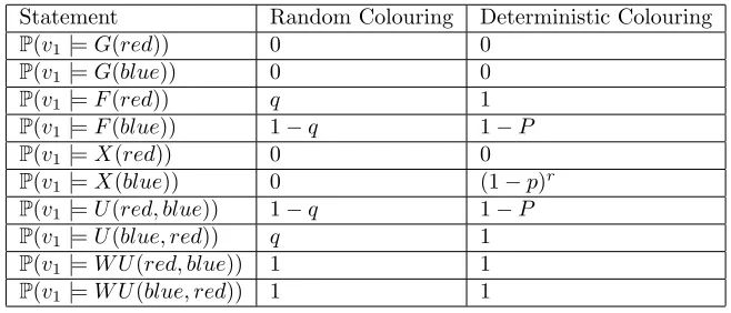
Now all the basic Linear Time Logic statements have been covered both us-ing the random vertex colourus-ing and the deterministic colourus-ing. The results are summarised in table 1. The most striking difference between the results using the different colouring methods, is the fact that the finite number of red states in the deterministic colouring method resulted in finite probabilities for certain model checking statements, while the probabilities of the random colour-ing either satisfied a zero-one law or were fully determined by the colour ofv1. Paradoxically the deterministic colouring was introduced in order to do an at-tempt to write Linear Time Logic statements in terms of First Order Logic statements. If that was possible, the results on zero-one laws as proved for First Order Logic might have been applicable to the Linear Time Logic statements of model checking. However the fixing of the number of red vertices caused the opposite. It let some probabilities depend on finite structures in the graph. Therefore some probabilities did not satisfy the zero-one law.
Statement Random Colouring Deterministic Colouring
[image:17.612.141.470.338.479.2]P(v1|=G(red)) 0 0 P(v1|=G(blue)) 0 0 P(v1|=F(red)) q 1 P(v1|=F(blue)) 1−q 1−P P(v1|=X(red)) 0 0 P(v1|=X(blue)) 0 (1−p)r P(v1|=U(red, blue)) 1−q 1−P P(v1|=U(blue, red)) q 1 P(v1|=W U(red, blue)) 1 1 P(v1|=W U(blue, red)) 1 1
Table 1: Probabilities of basic Linear Time Logic Statements
7
Conclusion
References
[1] Marcus M¨ulller-Olm, David Schmidt and Bernhard Steffen: Model-Checking, A Tutorial Introduction.
[2] P. Erd¨os and A. R´enyi: On the Evolution of Random Graphs.
[3] Saharon Shelah and Joel Spencer: Zero-One Laws for Sparse Random Graphs.
[4] Joel Spencer: The Strange Logic of Random Graphs.
[5] Alasdair J. Graham and David A. Pike: A Note on Thresholds and Connec-tivity.
[6] J. A. Bondy and U. S. R. Murty: Graph Theory With Applications
[7] Dirk van Dalen: Logic and Structure.
[8] R. Fagin: Probabilities on finite models,J. Symbolic Logicchapter 41 (page 50-58).
[9] Y. V. Glebskii, D. I. Kogan, M. I. Liogonkii and V. A. Talanov: Range and degree of realizability of formulas in the restricted predicate calculus,