On the control allocation of fully actuated and over actuated multirotor UAVs

(1)

On the Control Allocation of Fully-Actuated and

Over-Actuated Multirotor UAVs

R. (Rens) Werink

MSc

Report

Committee:

Dr.ir. P.C. Breedveld Dr.ir. J.B.C. Engelen R. Hashem, MSc Dr.ir. W.B.J. Hakvoort

January 2019 001RAM2019 Robotics and Mechatronics

EE-Math-CS University of Twente

(2)

Chapter 1 Introduction

1.1 Background

During the development of UAVs, large improvements have been made in the control of these vehicles. During the long history of control, several different methods of control have been used. Over the last decades, control of systems and in particular multi-rotor UAVs has shifted to purely software based control. This has opened a large amount of opportunity to implement even more complex control algorithms. This technological advantage has enabled many different types of UAVs to be introduced, each with their own advantages, limitations and novel designs. The current experience is that the application of control allocation in software has not yet reached the level of current research. The focus will be on control allocation, as control of UAVs is a far more investigated topic and very application-dependent.

1.2 Research problem

The problem that will be addressed in this thesis is that the current state of control allocation, both in control allocation algorithms and implementation in software, are not sufficient for projects in current research. By addressing these shortcomings, it should be easier and faster for researchers to implement correct control allocation in their research projects.

1.3 Research method

(6)

allocation in currently available software packages. From this investigation, it will be possible to find points where the software implementation of control allocation can be improved.

In addition to this investigation, the current range of solutions to the control allocation problem will be expanded by introducing an additional control allocation algorithm that will provide a solution to some systems that were not solvable with existing solutions in literature.

(7)

Chapter 2 UAV theory

2.1 UAV definition

As there exist many different types of UAVs (Unmanned Aerial Vehicles), a definition will be given of what types of vehicles are considered in this thesis. Figure 2.1 shows a classification of different types of UAVs, which are all single-body vehicles, i.e. all systems here are considered to consist of a single rigid base onto which all actuators are placed.

This thesis will focus on multi-rotor heavier-than-air vehicles, therefore all forces that are exerted on the body result directly from the actuators themselves, this is in contrast with systems that are equipped with control surfaces, such as planes.

[image:7.595.164.435.540.638.2]

As for interaction, it is assumed that the vehicle is completely free-floating, which means that there are no external forces (except gravity) acting on the system.

(8)

2.1.1 Actuation

The main method of propulsion is through the use of fixed-pitch propellers, actuated by brushless DC motors. Other control surfaces, such as wings or ailerons, are not considered. This has the advantage that the forces and torques acting on the UAV are not dependent on velocity, but only on actu-ator outputs.

To describe these forces and torques more easily, the concept of a wrench will be used. A wrench consists of the set of forces and torques acting on a body, in this case the UAV itself. As a single body has 6 degrees of freedom, the acting wrench on a UAV is also composed of 6 elements: three forces and three torques, as shown in equation 2.1. In a similar way, the position can be defined as a matrix H and the velocities as a twist T. [2]

W =

τ F

(2.1)

2.1.2 Sensory system

To control a multi-rotor UAV, sensors are included to measure the position, velocity and attitude of the vehicle. To measure the position and therefore the velocity, GPS can be used when flying outdoors, however, the accuracy is not good and GPS is unreliable. When flying indoors, other systems, such as OptiTrack can be used [3]. This measurement is based on infra-red cam-eras and indicators placed on the vehicle and therefore more accurate. An accelerometer is used to estimate the position as well, but as this involves a double integration, direct position measurements are more reliable. Mea-surements of the attitude of the vehicle are performed using a gyroscope and an accelerometer. State estimation techniques such as a Kalman filter can be used to further increase the accuracy of the measurements by using an internal model of the UAV and combining measurements of position and velocity.

2.2 Dynamics

To fully analyse the the behaviour of a UAV and therefore to understand the meaning of control allocation, the dynamics of a UAV are important to know. The main point is to understand how the actuator together produce a wrench on the system, and how this relation can be found.

(9)

UAV can be described separately. This can be done as each force generates a wrench around the centre of mass of the body, this is only dependent on the force vector and the position of the propeller relative to the centre of mass. Additionally, a torque will be generated opposite the rotational direction of the propeller. These can the be summed to find the total wrench acting on the body.

Wtotal =

nact

X

k=1

Wk (2.2)

By taking the Jacobian over the individual propeller thrusts, a linear description of the wrench can be found, which is the matrix M. This M

could still contain actuator outputs in the case of non-static UAVs, this will be explained in more detail later.

2.2.1 Rotor dynamics

The rotor itself is not an ideal system, to understand the limitations of the rotor, it must be understood that internally, there are some dynamics that influence the control of a multi-rotor UAV. Each propeller has a certain inertia and with the speeds that are used, the spin-up and spin-down times, which are an indication of the time it takes before a propeller is at its desired speed, are not insubstantial.

As a propeller rotates, it will experience drag as a result of friction with the air, this will result in a torque being generated in the opposite direction as the rotation of the propeller, this torque is linearly related to the rotational speed of the propeller through the drag-to-thrust coefficient γ.

Another point that shows up in the case of tiltable propellers is that gyroscopic forces will appear when rotating a propeller around a certain axis. This will influence the rate of change of the tilt of a rotor.

The force created by a propeller is also not linear with the rotational velocity of the rotor. This relation will depend on the rotors used, but generally follows a quadratic relationship. Due to this relation, only the output force λ will be considered in the analyses in this thesis.

2.3 UAV Classifications

(10)

[image:10.595.220.376.128.220.2]

Figure 2.2: Example of an underactuated quadrotor [4]

Different platforms can be classified using the mapping matrix M to define some strict boundaries between the classes. Equation 2.3 shows the relation between the output wrench W and the actuator outputs λ in case of a static system. M is the relation between these two and is assumed to be constant, any non-linear dependencies have been removed. From the rank of the matrix M, the classification of the UAV can be determined. In the case of a matrix multiplicationb=M·a, the rank of a matrix gives an indication of the dimension of the attainable set of b. For example, if the matrix has a rank of 3, it can produce a vector a in three dimensions, regardless of the sizes of vectors a and b.

W =M ·λ (2.3)

In the case of convertible systems, it must be noted that the classification as presented here that applies to the system will depend on the current pose of all actuators. Such convertible systems are not necessarily always in the same category.

2.3.1 Under-actuated

A system is considered under-actuated if the rank of the matrix M is less than 6, this means that the specific configuration of the actuators is not sufficient to fully actuate in all 6 dimensions of a full wrench, which is composed of three forces and three torques. To give an example of such a system, a standard quadrotor such as the one in figure 2.2 can be considered.

(11)

[image:11.595.220.374.126.244.2]

Figure 2.3: Example of an underactuated octo-rotor [5]

on the axis of the propeller given a certain thrust produced by that propeller.

M =        

L −L −L L

L −L L −L

γ γ −γ −γ

0 0 0 0

1 1 1 1

        (2.4)

The rank of this matrix is equal to 4, as two force components cannot be actuated. As this is less than the six required for actuation of the full wrench, it means that this system is under-actuated.

Some configurations will have more actuators, but will still be under-actuated. This is then due to the orientation of the propellers An example of this is the octorotor in figure 2.3, it has eight propellers, but as the force vectors are all parallel, it can only produce forces in one direction, making it an under-actuated system.

Additionally, the energy required to rotate a propeller is related to the rotational velocity of this propeller an d therefore quadratically related to the output force of a propeller. By spreading the required force over more propellers, the energy usage of a UAV can be lowered by installing more propellers.

The additional benefit of having eight rotors in this case is that four can be used for redundancy and it can therefore handle rotor failure or use this redundancy to lower the energy consumption by spreading the forces needed over all eight rotors.

(12)

[image:12.595.108.495.461.564.2]

Figure 2.4: Example of a fully-actuated hexarotor [7]

do not only need to generate the force required to keep the system afloat, but must also counteract the force applied sideways by the other propellers, therefore wasting energy that should otherwise not be needed.

2.3.2 Fully-actuated

A configuration is considered fully-actuated if the rank of the mapping matrix is equal to 6 and the number of actuators is equal to 6. An example of this is a hexarotor with tilted propellers [6]. The mapping matrix of such a system is given in equation 2.5, the tilting angle of the propellers (α) is in this case a constant value. For all values of α 6= k · π

2, this matrix has rank 6 and therefore the system is fully actuated.

M =        

cαL −cαL −1₂cαL ₂1cαL 1₂cαL −1₂cαL

0 0

√ 3

2 cαL −

√ 3 2 cαL

√ 3

2 cαL −

√ 3 2 cαL

γ+sαL −γ−sαL γ+sαL −γ−sαL −γ−sαL γ+sαL

−sα −sα

√ 3 2 sα

0 0 1

2sα

1

2sα −

1

2sα −

1 2sα

cα cα cα cα cα cα

        (2.5) Herecα = cos(α) and sα = sin(α) for readability

A special case within this category is an omni-directional system, this is the case if the combined set of all attainable forces, which are the last three elements of the wrench, can support the weight of the vehicle in all directions. This allows the vehicle to sustain flight in all possible orientations.

(13)

[image:13.595.138.475.131.229.2]

(a) Voliro [11] _{(b) Large quadrotor [12]}

Figure 2.5: Vehicles having integrated control allocation

2.3.3 Over-actuated

If a configuration has a full rank, i.e. rank(M) = 6, mapping matrix and the number of actuators is larger than 6, it is considered over-actuated. It has the same properties as a fully-actuated system, but has a larger freedom in the control allocation due to the redundant actuators. This redundancy is again useful for fault-tolerancy and energy-efficiency. However, a lot of the time, this extra actuation is a result of tilting propellers, which allow the UAV to change the force vectors that act on the system. By changing its configuration, a UAV is capable of fingin

2.4 Static and convertible systems

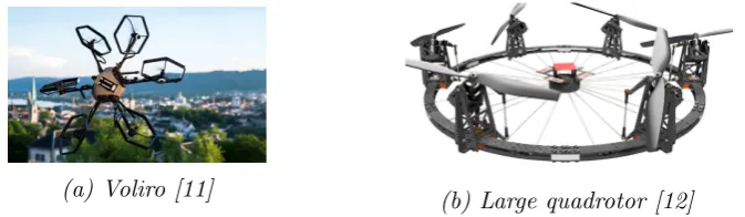
Some multi-rotor systems have propellers that can change the angle under which the force is applied to the system, for example by using a servo motor to rotate the motor that drives the propeller. This is for example used in the Voliro [11] and the FAST-Hex [12], these can be seen in figure 2.5.

In the case of a convertible system, the matrix M will not be a static matrix, but is dependent on the tilting angle of the individual rotors. This means that the relation between the actuator forcesλand the output wrench

(14)

Chapter 3 Control allocation theory

3.1 Application of control allocation

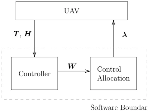
To understand why control allocation is used and what it is, first the general structure of a control system should be understood. A control system is used to monitor and control a given system. This is done by interfacing a controller to the system using sensors to get information about the state of the system and actuators to influence this system. Schematically, this structure is given in figure 3.1.

UAV

Controller Control

Allocation

T, H

W

λ

[image:14.595.172.410.443.621.2]

Software Boundary

Figure 3.1: General communication diagram.

(15)

To find the required actuator outputs to create this desired wrench, a second block is added which is the control allocation. The implementation of this is highly dependent on the configuration of the UAV.

By separating these two tasks, the implementation of different controllers becomes much easier, as the configuration and individual actuators do not need to be considered as the interface between the different blocks is defined as only a wrench.

3.2 Control allocation problem

The main problem in control allocation is the transformation of a desired wrench into individual motor commands. To do this, a combination of all actuator outputs has to be found that results in the desired output wrench and optimally distributes this over all individual actuators.

Given the general equation that describes the relationship between the actuator outputs λand the output wrenchW: W =M(λ). The control al-location problem is to find the inverse relationship between these two vectors. This can be a very difficult task, as M(λ) could be any function that links these two. In general the solution is a function or algorithm dependent on the desired wrench that produces the required actuator outputs: λ=M∗(W).

That is to say, to find an optimal relation between a desired wrench and the individual actuator outputs. This M∗ can be anything from a static matrix to a multi-step algorithm. The actual solution will depend on many factors including actuator configuration, non-linearity and actuator limits. Before solving this problem, it first needs to be understood that there are different classifications of drones, which all have their own properties and special cases.

Solutions to the control allocation problem are based on an optimization over all actuators while producing the desired output wrench. This means that the desired wrench is attained while considering actuator properties, this can be their limitation, a preferred output value or weights can be placed on the individual actuators.

3.2.1 Actuator limitations

(16)

Chapter 4 Control allocation solutions

4.1 Introduction

As the implementation of the control allocation is highly dependent on the configuration of the UAV, there are many different solutions to the control allocation problem. To find out what the most commonly used solutions are, a literature survey was performed to compare the algorithms used in current research. The next section will describe the different solutions, how they work and what research projects use that implementation. [13].

After this survey, a summary of the different solutions and the number of times they have been used will be presented.

4.2 Literature survey

4.2.1 Integration in controller

In situations where the configuration of a platform is fixed and a controller is designed for this specific configuration, a good solution is to inherently include the configuration of the UAV into the controller, this controller will then return the desired actuator forces λ. This approach is used in several projects that mainly focus on hardware design. These are for example a miniature quadrotor [14] and a large quadrotor [15], which can be seen in figure 4.1.

(17)

(a) Micro indoor quadrotor [14]

[image:17.595.317.473.144.269.2]

(b) Large quadrotor [15]

Figure 4.1: Vehicles having integrated control allocation

(a) Unusually shaped fully

actuated hexarotor [8] (b) Fully actuated hexaro-_{tor [7]}

(c) FAST-Hex tiltable

hexarotor [12]

Figure 4.2: Vehicles using the matrix inverse

4.2.2 Matrix Inverse

In the case where the number of actuators is equal to the number of degrees of freedom of a platform, the mapping matrix M is a square matrix. If this matrix is directly invertible, which means that no singularities can occur in this system, the optimal and only solution to the control allocation problem is to take the inverse of the mapping matrix as the control allocation matrix:

λ=M−1Wdes

[image:17.595.106.495.339.443.2]

(18)

4.2.3 Moore-Penrose pseudo-inverse

A simple solution to the control allocation problem is the Moore-Penrose pseudo-inverse. The pseudo-inverse tries to solve an unconstrained control allocation problem. For a given system of the formW =M λwith staticM, a quadratic cost has been placed on the deviation of the actuator output from its preferred value multiplied by a weighting factor, as is shown in equation 4.1. By minimizing this cost function, the optimal values for the actuator outputs can be found.

Cost = 1

2(λ−λp)

T_D₍_λ₋_λ

p) (4.1)

In the case that B is full rank, or equal to the number of degreees of freedom, the general solution can be given by:

λ= (I −CM)λp+CD (4.2)

where

C=D−1MT(M D−1MT)−1 (4.3)

In these equations, D is a diagonal weighting matrix for the individual actuators. λp are the preferred values for the actuators.

If it is assumed that the preferred output value for all actuators is zero and the weighting for all actuators is equal, as is the case for most general multirotors, the solution can be simplified to the form:

λ=CW (4.4)

where

C =MT(M MT)−1 (4.5)

This final C is what is known as the pseudo-inverse.

(19)

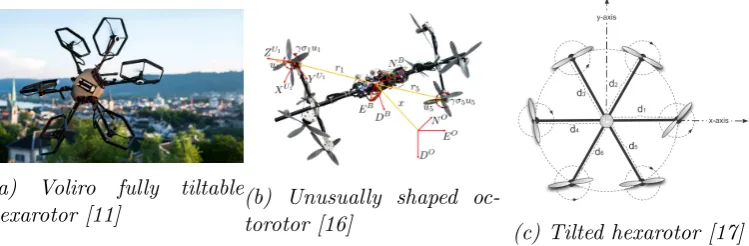
(a) Voliro fully tiltable

hexarotor [11] (b) Unusually shaped oc-_{torotor [16]}

[image:19.595.111.486.133.256.2]

(c) Tilted hexarotor [17]

Figure 4.3: Vehicles using the Moore-Penrose pseudo-inverse

fault tolerancy, where the failure of an actuator causes the system to become under-actuated. In both of these cases it is necessary to use the pseudo-inverse. This UAV can be seen in figure 4.3c.

The Voliro [11], which is an over-actuated hexarotor, uses the Moore-Penrose pseudo-inverse for the control allocation, but as this system uses tiltable rotors and therefore a non-static mapping matrix, addition processing is needed. This will be explained in more detail in section 4.2.5.

4.2.4 Redistributed pseudo-inverse

A limitation of the Moore-Penrose pseudo-inverse is that it assumes an un-constrained output of the actuators, which is rarely the case.

To try to solve this problem of actuator limitations, the redistributed pseudo-inverse method was created. This method starts by performing a regular pseudo-inverse, but then continues to identify actuator outputs that have been saturated and will try to redistribute the missing part of the de-sired wrench by altering the remaining, unsaturated actuator outputs. This redistribution can be repeated until a satisfactory result is obtained. In some cases, an optimal result cannot be found, but the wrench error can be mini-mized using this approach.

The redistributed pseudo-inverse works as follows: [13]

1. Start by performing a pseudo-inverse on the unconstrained system:

λ=B†·W

2. Due to constraints, the actual outputs are a projection onto the allow-able set λ¯ = Proj(λ).

3. The next step is to decompose the constrained output into a constrained and an unconstrained part: λ¯ = (λ¯T

(20)

4. A similar decomposition will be performed on the mapping matrix M:

M = (MC,MU)

5. The wrench as generated by the saturated output is found next: WC =

MC·λ¯C

6. The remaining wrench is then attempted to be generate using the un-constrained actuator outputs: MU ·λU =Wdes−WC

7. This algorithm is then repeated until a solution is found or no further improvements can be made

In literature, the redistributed pseudo-inverse is used in [18], which presents a fault-tolerant octorotor. In this case the researchers have chosen to include actuator saturations into their control allocation, which lead to the redis-tributed pseudo-inverse being used in this research

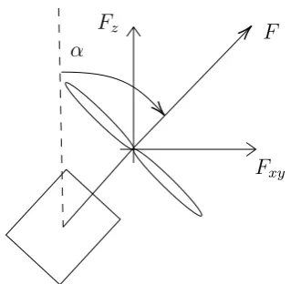
4.2.5 Force decomposition

The inverse and pseudo-inverse are only applicable to static systems, To solve the control allocation problem for convertible systems, additional methods have to be used. A common actuation method used in convertible systems is a tilting rotor, such as is used in the Voliro [11] and the FAST-Hex [12]. These systems have rotors that can be moved by using servo motors to change the direction of the thrust vectors.

A general way of solving the control allocation problem that is introduced by tilting rotors is to transform the polar force description that uses the physical outputs of the actuators to a form using Cartesian coordinates. The polar force description is a result of the two actuators that make up the tilting system, which is a standard propeller producing a force F and a servo that rotates this thrust around an angle α.

This decomposition is visualised in figure 4.4. Here,Fz is directed in the

upwards vector of the body-fixed frame, Fxy is directed in the x-y plane of

the body-fixed frame of the system.

Fxy = sin(α)·F (4.6)

Fz = cos(α)·F (4.7)

This transformation will result in a mapping matrix that is again linear inFx andFy, such that it can be solved with more general control allocation

(21)

Fz

Fxy

[image:21.595.215.375.125.281.2]

α F

Figure 4.4: Definition of force decomposition

into a polar force description, as this is the information that can be used by the actuators.

This is also the solution used in the Voliro project [11], where an inde-pendently tiltable fully-actuated hexarotor is presented. As the force decom-position is performed, the mapping matrix becomes a 6 by 12 linear matrix, which is then used with the Moore-Penrose pseudo-inverse to find the con-trol allocation solution. To give an idea of how this approach works, the non-linear mapping matrix of the Voliro is given in equation 4.8

M(α) =

        

cα1L −cα2L −1₂cα3L ₂1cα4L 1₂cα5L −1₂cα6L

0 0

√ 3

2 cα3L − √

3 2 cα4L

√ 3

2 cα5L − √

3 2 cα6L

γ+sα1L −γ−sα2L γ+sα3L −γ−sα4L −γ−sα5L γ+sα6L

−sα1 −sα2

√ 3 2 sα3

√ 3 2 sα4

√ 3 2 sα5

√ 3 2 sα6

0 0

√ 1 2 sα3

√ 1

2 sα4 −

√ 1

2 sα5 −

√ 1 2 sα6

cα1 cα2 cα3 cα4 cα5 cα6

(22)

Decomposed, this becomes the following 12 by 6 matrix: M =         

0 L 0 −L 0 −1

2L 0

1

2L 0

1

2L 0 −

1 2L

0 0 0 0 0

√ 3

2 L 0 −

√ 3

2 L 0

√ 3

2 L 0 −

√ 3 2 L

γ+L 0 −γ−L 0 γ +L 0 −γ−L 0 −γ−L 0 γ+L 0

−1 0 −1 0

√ 3 2 0 √ 3 2 0 √ 3 2 0 √ 3 2 0

0 0 0 0

√ 1

2 0

√ 1

2 0 −

√ 1

2 0 −

√ 1

2 0

0 1 0 1 0 1 0 1 0 1 0 1

         (4.9)

The corresponding lambdas are in this case:

λ= (λ1,xy, λ1,z, λ2,xy, λ2,z, λ3,xy, λ3,z, λ4,xy, λ4,z, λ5,xy, λ5,z, λ6,xy, λ6,z)T

Due to this approach, control for the convertible Voliro can be allocated using standard linear methods.

4.2.6 Search algorithms

Reference [19] presents a multirotor UAV designed by an optimization algo-rithm on the configuration of the rotors, therefore the amount of propellers and their orientations are unknown. An example of this system can be seen in figure 4.5. The approach used in this paper is to use a generalized pattern search to find the optimal distribution of actuator outputs. This method was probably chosen as the number of rotors and their positions are unknown or constantly changing.

In general, search algorithms can be used for all different control alloca-tion problems, as it will try to iteratively find the optimal solualloca-tion for all actuators. It is however rarely used as it has a great computational disad-vantage over all other solutions.

4.3 Literature summary

To effectively compare the different solutions, their use cases will now be presented in table 4.1.

(23)

[image:23.595.162.435.135.300.2]

Figure 4.5: A computer generated hexarotor [19], this vehicle uses a search algorithm to find the solution to the control allocation problem

Solution Usage Count

Integration in con-troller

This method is mostly used in research that is not directly focussed on control and does not have an explicit control allocation loop.

2

Matrix inverse This is the easiest method for separated control allocation, it is used in cases where the number of actuators is equal to the number of degrees of freedom.

3

Moore-Penrose matrix inverse

This is an optimised solution that can be applied on vehicles that have a different number of actu-ators compared to the numbers of freedom.

3

Redistributed pseudo-inverse

In cases where actuator limitations should be con-sidered, this method can be used as an extension on the Moore-Penrose pseudo-inverse.

1

Force decomposi-tion

For systems with independently tilting rotors, this method can be used to create a static control al-location problem, which can be solved with the above methods.

1

Search algorithms In cases where the above methods are not appli-cable, this method can be used to iteratively find the optimal solution for the actuator outputs, it is very computationally intensive.

1

[image:23.595.102.530.362.688.2]

(24)

(25)

Chapter 5 New control allocation

algorithm

5.1 Design requirements

From the comparison of the different control allocation algorithms in chap-ters 4, it was concluded that there is a large step between using the force de-composition method, which can control systems with independently tiltable propellers and the application of a dynamic search algorithm. To show how a new algorithm can help in this context, the control allocation solutions of the Voliro [11], which is an independently tiltable hexarotor and the FAST-Hex [12], a hexarotor with coupled tilting propellers will be compared

5.1.1 Comparison between 12DoF and 7DoF control

allocation

As discussed in chapter 4, a tiltable rotor can be decomposed into a vertical and horizontal component. Applying this to the Voliro [11] creates a 12 by 6 mapping matrix that can be solved with the Moore-Penrose pseudo-inverse and by reverse mapping the output signal can be found.

This method will not work for the FAST-Hex, of which the mapping matrix is given in equation 5.1. Trying to apply the same technique will transform the originally 7 degrees of freedom of the actuators into 12 degrees of freedom and will disconnect the six tilting angles, which is not possible. The solution proposed by the original paper is to allow the pilot to choose the tilt angle.

(26)

[image:26.595.164.430.139.261.2]

Figure 5.1: Diagram of the FAST-Hex construction [12]

such systems, a new algorithm will be presented.

M(α) =

       

c αL −c αL −1

2c αL 1 2c αL

1

2c αL −

1 2c αL

0 0

√ 3

2 c αL −

√ 3 2 c αL

√ 3

2 c αL −

√ 3 2 c αL

γ+s αL −γ−s αL γ+s αL −γ−s αL −γ−s αL γ +s αL

−s α −s α

√ 3 2 s α

0 0 1₂s α 1₂s α −1

2s α −

1 2s α

c α c α c α c α c α c α

        (5.1) Herec α= cos(α) ands α= sin(α) for readability

5.2 Approach

To solve the control allocation problem of the FAST-Hex, a hybrid solution is proposed that uses the Moore-Penrose pseudo-inverse for the main control allocation and a separate search algorithm to find the optimal tilt angle. By combining these, the angle can be adjusted to find the optimal propeller output. The algorithm works as follows:

1. Given a system that can is linear in λ and where the mapping matrix is only dependent on a single α. The dynamic equation can be written as W =M(α)λ.

(27)

3. To find an optimal value for the tilt angle α, a cost function is intro-duced on the propeller forces λ. This cost function is free to choose and can be used to address limitations on the actuator.

4. By minimizing this cost function, an optimal value of the tilt angle α can be found. By choosing an appropriate minimization algorithm or by limiting the allowed change in angle, limitations on α itself can be included, this will be explained in the next section.

This minimization does not have to be performed at every control allo-cation step, as only the first two steps are necessary to find a solution to the control allocation problem and can use a previously determined tilt angle. This property of the algorithm could be used if computational load is an important factor: by limiting the amount of angle optimization steps, com-putational load can be reduced, this should be done carefully, as it could lead to non-consistent loop timing.

5.2.1 Cost function

An easy cost function that can be used to optimize the tilt angle is to take the sum of the square of the output forces, as is described in equation 5.2. In this case, λ(α) is a function that describes the actuator forces as a function of α and is a result of the pseudo-inverse of the mapping matrix.

Cquadratic(α) =

nact

X

k=1

λk(α)2 (5.2)

This can be seen as putting a cost on the energy use of the actuators and by taking this cost function, the most energy efficient tilt angle can be found while also getting the required actuator output. This is also the same cost function as used by the Moore-Penrose pseudo-inverse to get the optimal output

There are limitations on what cost functions can be chosen for this pur-pose. The main criteria are that it is a continuously differentiable function with no local minima, the derivative of this function should also always have a finite value at all possible values of the output. This will allow the opti-mization algorithm to find the global optimum for the tilt angle.

5.2.2 Actuator limits

(28)

-6 -4 -2 0 2 4 6

Actuator output (N)

0 20 40 60 80 100

Cost

Cost functions

[image:28.595.169.411.131.281.2]

Quadratic cost Lower limit

Figure 5.2: The two cost functions as a function of the exerted force

attainable force or the fact that a UAV is fitted with unidirectional propellers and therefore cannot produce negative thrusts.

This can be taken into account while choosing a cost function by shaping it such that an additional cost is placed on unattainable forces, this will not prevent the control allocation algorithm to use these force sets, but the use is heavily penalized. This should help the control allocation algorithm to choose the angle α such that the actuators are within their allowed range.

To test this with an example, when an actuator cannot produce negative thrusts, an additional weight should be placed on the negative forces. The cost function that has been chosen for this is given in equation 5.3.

Climit(α) =

nact

X

k=1

(λ2_k+e−λk₎ _(5.3)

Plotting these cost functions against λ result in the plot in figure 5.2. It can be seen that this new cost function is similar to the previous cost function in the positive force range, but shows exponential behaviour towards the negative force range, which should discourage the optimization from choosing negative actuator outputs.

To test the functionality of this new cost function, a simulation will be performed in cases where it will reach the lower force limit

5.2.3 Tilt limits

(29)

to physical limits and the tilt rate. The rate is limited as the time it takes for the tilt to change is relatively high. This is mostly caused by a combination of a large inertia in the system, friction and the gyroscopic effects that will appear when tilting spinning propellers.

Both of these limits can be solved by adapting the search algorithm, by implementing either global limits to limit the angle itself and a limit on the allowable change to limit the rate of change. How the algorithm works under different limits of the angle will be investigated in the simulations.

5.3 Simulations

To test the ability of the algorithm to work with the limits on the actuators, a simulation has been performed in 20-sim [20]. The trajectory taken in this simulation was chosen such that the lower limit on the rotors would be reached, which is where the difference between the cost functions is expected to show.

The particular trajectory used for the comparison between the different cost functions is a vertical circular trajectory. To compare the two cost functions, the UAV will be asked to trace this trajectory with different radii and increasing radial velocity. At some point the UAV will become unstable and fail to follow the trajectory.

Expected is that the cost function that takes into account the lower limit will be able to work at a higher radial velocity compared to the cost function that is ignorant to the actuator limits. The limits for the angle have been set to ±90◦, such that they would not influence this simulation.

(30)

1.5 2 2.5 3 3.5 4 4.5 5

Radius of trajectory (m)

5 10 15

Angular velocity (rad/s)

Failure points with vertical trajectory

[image:30.595.172.410.130.281.2]

Figure 5.3: Failure points on a vertical trajectory

Next, it is interesting to also compare how the different algorithms han-dle limitations on the tilt angle, for that purpose, simulations have been performed where the angle was limited to ±45◦ and 30◦ from the under-actuated position. These values were chosen to be around the values that the algorithm used in the unconstrained case and that the limits would be hit. However, the system would still be able to fly while using these limits.

The results of the simulation with a limit of±45◦ can be found in figure 5.4. Here, the same behaviour can be observed with an average increase of around 20% in angular velocity.

3 3.5 4 4.5 5

6 8 10 12

Failure points with horizontal trajectory and angle limit of 45

Figure 5.4: Failure points on a horizontal trajectory and a limit of 45 deg

[image:30.595.172.423.470.622.2]

(31)

the UAV. The difference that the control allocation can make is in also quite limited, as the optimal angle is beyond the limits that have been set.

2 2.5 3 3.5 4 4.5 5

4 6 8 10

Failure points with horizontal trajectory and angle limit of 30

[image:31.595.171.424.172.323.2]

Figure 5.5: Failure points on a horizontal trajectory and a limit of 30 deg

When comparing the actual actuator outputs from a simulation, such as the outputs in figures 5.6 and 5.7. These figures are the outputs for an equal vertical trajectory with a radius of 3.5m and a angular velocity of 3.8, which is well within the stable region of both cost functions. It can clearly be seen that the asymmetrical cost function that uses the lower limit has significantly less outputs in this negative range while the tracking error is mostly similar. To compensate for the reduced negative output, the positive side of the outputs has been increased slightly, but from the simulations it can be seen that this is not a significant increase.

10 15 20 25 30 35 40 45 50

Time (s)

-15 -10 -5 0 5 10

Desired output (N)

Output 1 Output 2 Output 3 Output 4 Output 5 Output 6

[image:31.595.135.459.512.690.2]

(32)

10 15 20 25 30 35 40 45 50

Time (s)

-6 -4 -2 0 2 4 6 8

Desired output (N)

[image:32.595.138.458.140.320.2]

Output 1 Output 2 Output 3 Output 4 Output 5 Output 6

Figure 5.7: Actuator outputs with the asymmetrical cost function

5.4 Conclusion

From the literature survey on control allocation solutions, it became clear that there was room for an algorithm that could solve the control allocation problem for systems that do not have fully independent actuators but where a dynamical search algorithm is too advanced. As an example, the full control allocation of the FAST-Hex has been used.

By using a hybrid solution of both the Moore-Penrose pseudo-inverse and a search strategy, an algorithm was created that could use the output of this pseudo-inverse to optimize the remaining actuator outputs. In this case, the shared tilting angle was optimized.

Another point that was implemented with this algorithm was the possibil-ity of implementing limits of the actuator outputs into the control allocation. This was done by altering the cost function on the actuator outputs to apply a greater cost on the unattainable part of the output forces. Optimizing the tilt angle by minimizing the cost function will lead to the actuator outputs to shift towards the attainable force region and therefore minimizing the output wrench error.

(33)

(34)

Chapter 6 Control allocation in software

6.1 Introduction

In research, it is common to include the control allocation in a software package that is responsible for the control system of the UAV. To create a functional system for current research, an analysis of the limitations of current software packages can be performed.

There are several different software packages that can be used to control UAVs. These include for example the ArduPilot [21], LibrePilot [22] and the PX4 control software of the Dronecode project [23].

For the investigation of the UAV control software, one package will be chosen and analysed. For this project, this will be the PX4 software package, as it is open-source and the design principles have also been published [24], therefore the code can be analysed easily. Additionally, as it is currently in use in the research environment, there is already some knowledge about this software package within the research group and the adapted version can easily replace the current solution.

In this chapter, the PX4 system will be investigated to find points of improvements to make the software more applicable in current research.

6.2 Software structure

(35)

run independently. This has the advantage that controllers can run at dif-ferent loop speeds and priorities, it also allows for modules to be substituted by similar modules with different implementations. This system is visualised in the diagram in figure 6.1.

uORB communications layer

[image:35.595.181.410.200.275.2]

Module Module Module Module

Figure 6.1: PX4 system architecture

6.3 Software goals

To find what needs to be improved in the software, some goals are defined for what the software should be capable of to allow for efficient research. These goals will be set within the current framework of the software. The two main points that will be considered are the communication and the implementation of the modules.

6.3.1 Communication

To allow for predictable communication between the different modules in the software, it is important that all topics are clearly defined and physically accurate. It is then also important that the values sent through the topics are correctly scaled, such that a module that uses these values can use them as absolute truth and does not need to perform any additional scaling. By implementing this, the software will provide a clear interface between the modules.

(36)

6.3.2 Modules

To allow for a versatile software package, the included modules should be applicable for various different cases. For example, an under-actuated UAV uses very different controllers and control allocation algorithms compared to a fully-actuated or over-actuated system. To allow for various different configurations, different modules should be included that can be picked and activated whenever it is necessary for the correct functioning of the system. As a start, the most common approaches should be available to researchers.

6.4 Software analysis

(37)

UAV

Position Controller

Attitude Controller

Control Allocation

H,T

Software Boundary

λ

τ

Fz

Rdes

[image:37.595.146.451.267.533.2]

H,T

(38)

6.4.1 Controllers

Within the software, control of the UAV has been split into a position con-troller and an attitude concon-troller, which are also decoupled within the soft-ware itself. This also allows both to run at different loop speeds and perform a specific task.

Position controller

The position controller consists of two main parts, a PID controller and a force projection. The PID controller uses the position error to create a velocity setpoint vsp = rsp −rˆ, this velocity setpoint is subsequently used

to calculate the velocity error, which is used as an input into another PID controller to produce the desired acceleration. As the system is at this point agnostic about the physical properties of the UAV, this acceleration is used as a desired force vector.

The next step is to transform this desired force vector into a single up-wards force and an attitude to recreate the desired force vector. This step is performed as the software assumes an under-actuated system and requires the vehicle to tilt in order to generate .

Attitude controller

The role of the attitude controller is to generate a desired torque to steer the vehicle to the desired attitude as generated by the position controller. The reason that this controller is separated from the position controller is because the attitude controller needs a higher update rate compared to the position controller because of the unstable nature of a multi-rotor UAV. It can then match the update rate of the gyroscope to create accurate outputs.

6.4.2 Mixer / Control allocation

The next step is the control allocation or mixer, as it is called within the PX4 software. This implements a pseudo-inverse mixing using a previously generated 4xN ’mixing matrix’, which is the inverse of the mapping matrix

M as shown in chapter 3.

The mixing matrix in the current implementation of the software is a normalized matrix, which means that it is independent of the physical prop-erties of the vehicle. To show how such a matrix is composed, the mapping matrix M of the quadrotor in equation 2.4 will be used.

(39)

[image:39.595.218.377.128.283.2]

Figure 6.3: Configuration of a standard quadrotor [25] M =    

L −L −L L

L −L L −L

γ γ −γ −γ

1 1 1 1



  

(6.1)

To create a normalized matrix, this mapping matrix will be split into a diagonal matrix that contains all parameters and an additional matrix that will only contain constant values. The decomposed matrices can be seen next

M =



  

L 0 0 0

0 L 0 0

0 0 γ 0

0 0 0 1

       

1 −1 −1 1

1 −1 1 −1

1 1 −1 −1

1 1 1 1



  

(6.2)

To find the mixing matrix, the inverse of this matrix will be taken:

M−1 =



  

1 1 1 1

−1 −1 1 1

−1 1 −1 1

1 −1 −1 1

        1

4L 0 0 0

0 ₄1_L 0 0 0 0 ₄1_γ 0

0 0 0 1₄



  

(6.3)

(40)

Base Mixer

Mixer Group Helicopter Mixer

[image:40.595.139.457.127.345.2]

Multirotor Mixer

Figure 6.4: Class structure of the mixers in the current implementation.

6.4.3 Mixer class implementation

The way it is implemented in the code is such that different control allocation methods can be used simultaneously . Several different mixer classes have been created, which are all based on a single base mixer. These mixing classes can then be combined into a so-called mixer group, which defines which mixers and in which order they are executed. The structure of this can be seen in figure 6.4. This structure directly relates to the C++ implementation in the software itself, where each mixer class is derived from the base mixer class.

The different mixers have access to the control groups that are defined within the PX4 software, these channels contain all information that has to be sent to the UAV, including the desired output wrench of the actuators. This desired wrench is used by the defined combination of mixers to produce the various actuator outputs.

6.5 Conclusion

(41)

6.5.1 Control system

From the analysis of the controller and the control allocation, it was found that the software was designed for under-actuated systems. This was evi-dent from the implementation of the position and attitude controller, which together produced a desired wrench of only 4 elements (a single force and three torques). To be able to fly a fully-actuated or over-actuated UAV, the controllers should be able to output a full 6-element wrench to the control allocation.

In turn, the control allocation should also be able to handle this new im-plementation. Currently, it is also designed to only consider under-actuated UAVs. To mitigate this problem, the communication towards the control allocation should be redefined, but more importantly, the implementation of the control allocation has to be altered. The new implementation should be able to handle configurations that have forces in 3-dimensional space instead of only in the z-direction. In line with the software goals set, this new im-plementation should be implemented alongside the existing control system in the PX4 software.

6.5.2 Normalized signals

Between the controllers and the control allocation, the communication signals are normalized to a value between 0 and 1. This is a result of creating a system that will function for every system in its supported range. The signals will be the same between UAVs of different sizes. Individual vehicles are optimized by tuning the PID controller itself instead of changing the physical parameters of theses vehicles.

After mixing, the output is given as a value between 0 and 1 for the PWM signal. This value comes directly from the mapping matrix, but this hides a step that should have been taken. The output signal is sent to the ESC (electronic speed controller) on the vehicle and is directly related to the rotational velocity of the propeller. However, as described in chapter 2, the output of this matrix should be the thrust generated by the propeller. Due to experiments done on the relation between the rotational velocity and the output thrust, it has been found that this mapping is closer to a quadratic relation. The assumed linear relation is therefore not accurate.

(42)

Chapter 7 New software implementation

7.1 Required changes

As stated in the previous chapter, there are two main points that need to be improved. The first is that the current software does not support fully-actuated UAVs in its control, the second point is that it currently uses nor-malised signals in the communication instead of signals with physical mean-ing.

In this chapter, the steps needed to improve these two issues will be presented and the implementation of one of these changes will be executed and tested.

7.1.1 Intermodular communication

Considering the communication in the flight stack of the software, as de-picted in figure 6.2, the following observations can be made when trying to implement the physics based communication.

To implement the non-normalised signals, the signals do not need any updating as the size of the communication channels will not change. Most of the work will be performed in the conversion of controllers, mixers and other modules to use the new signal definitions.

After this, additional changes can be implemented that would increase the physical accuracy of the system. For example, the signals coming from the mixer can now be interpreted as a desired force and be translated by another module or implementation to calculate the required rotor velocity to get this force.

(43)

UAV

Position Controller

Attitude Controller

Control Allocation

H,T

Software Boundary

λ

τ F

Rdes

[image:43.595.145.451.121.391.2]

H,T

Figure 7.1: Communication diagram of the modified firmware.

7.1.2 Support for fully-actuated and over-actuated UAVs

To support fully-actuated systems, the flight control stack requires additional changes.

In the controllers, the output is no longer a reduced 4-element wrench, which only contains the upwards thrust, but the mixer will expect a full 6-element wrench with a full force vector. This requires changes to the con-trollers, as the additional input should be taken either from the operator or from an additional algorithm. For testing purposes, a simplified control structure can be used to show the correct operation of the new flight stack. The update communication diagram can be seen in figure 7.1.

(44)

Base Mixer

Mixer Group Helicopter Mixer

Multirotor Mixer

[image:44.595.140.460.128.431.2]

Complex Mixer

Figure 7.2: Structure of the mixers in the adapted software.

7.2 Implementation

To implement these changes, the code structure itself had to be altered. This was done to allow backwards compatibility with previous implementations. This is necessary as the controller for an under-actuated UAV is fundamen-tally different from one that is designed for fully-actuated UAVs. For the new implementation, two new controllers and an additional mixer have been created within the software package. Due to the modularity of the soft-ware, these can coexist with the previous controllers without any problems or compatibility issues.

A new mixer class, which has been called the ’Complex mixer’, will be derived from the base mixer class, as is the case for all existing mixers. This is done to be able to quickly switch between implementations to compare the behaviour. The addition of this new mixer will expand the class structure of the mixers to the situation in figure 7.2.

(45)

mixer class used for multirotor systems. The only difference is that the complex mixer will use a 6 by N mixing matrix instead of the previous 4 by N. The additional x- and y-forces have been mapped to 2 unused channels used in the communication between the controllers and the control allocation. The mixing matrices are created while building the software using a python script. This script uses the rotor position definitions for each sup-ported platform and creates a mapping matrix from this information. The mixing matrix is then created by taking the pseudo-inverse of this mapping matrix. The advantage of this approach is that control allocation is now only a matrix multiplication, which greatly improves the computational complex-ity of the system.

This script required an extension to create 6 by N mixing matrices re-quired by fully-actuated control allocation, but it should also still output the original 4 by N mixing matrices for the previous under-actuated control allocation.

For now, the mixer only accepts the 6-element wrench as an input, this re-quires all implementations of control allocation algorithms to be self-contained. Which means that the algorithms should only expect a desired wrench and produce the individual actuator commands. If additional inputs are required for a correct functioning of a control allocation algorithm, they should first be implemented in the code and made available to other modules or the pilot itself.

A more detailed overview of the changes made can be found in appendix A.

7.3 Results

To test the new implementation of the control allocation, the system was tested using a simulation in Gazebo [26] where the software is expected to try to fly several different UAVs. A constant attitude setpoint will be sent to the attitude controller while using the full available force-space to move the UAV, it is expected that the system would still be able to keep the UAV stable in flight, but that lateral movement would not be observed if a set-point change was introduced. Only when a fully-actuated system is implemented, would lateral movement be possible.

7.3.1 Controller changes

(46)

(a) Under-actuated quadrotor

(b) Under-actuated hexarotor

[image:46.595.117.476.129.263.2]

(c) Fully-actuated hexarotor

Figure 7.3: The different platform during a simulation in Gazebo

controllers were also changed in separate modules, to allow easy switching between the two controller implementations.

As stated in the previous chapters, the position controller performed two tasks, which were the actual control and a mapping for under-actuated con-trol. In the new system, this second task was bypassed and all three control forces were sent to the attitude controller together with a constant setpoint for the attitude.

The attitude controller was kept the same, except that it had to forward two more forces to the mixer.

When applied to under-actuated UAVs, it is expected that the software is able to keep the flight stable as the attitude controller has not changed. How-ever, as this new position controller will not tilt the UAV to move sideways, it will not be able to hold it in position but drift around uncontrolled.

This new control system should be able to fly a fully actuated UAV cor-rectly, that means that it should fly stable and be able to hold position.

7.3.2 Results

The system has been tested with three different UAVs, all of which can be seen in the simulation in figure 7.3

1. An under-actuated quadrotor

2. An under-actuated hexarotor

3. A fully-actuated hexarotor

(47)

their absolute position as the controller uses forces that are not attainable by these systems. They would simply drift around as corrections were also communicated through these unattainable channels. This shows that the controller is indeed only using the three forces to move the vehicle and the controller implementation was successful.

When simulation the fully-actuated system, it was observed that the under-actuated control allocation could not hold this system in a stable po-sition, which is a result of the two additional forces not being communicated. The fully-actuated control allocation was however successful in flying this system.

7.4 Conclusion

From the analysis of the PX4 software package two main improvement points were found that would enable the software to be more readily available for research purposes. By implementing these changes, it will be easier and more straightforward for users of this package to adapt it to their particular needs. The first point that was found was that the communication between the different modules is not based on any physical basis. To allow for predictable messaging and a clearer interface between the different modules, the commu-nication has to be altered software-wide to allow for more specific modules to be implemented.

The second improvement point is that the current iteration of the PX4 software only supports under-actuated multirotors. This change was im-plemented by altering the communication towards the control allocation to allow for a full wrench to be transmitted. Additionally, the control allocation module was altered to be able to process this desired wrench and to use the existing UAV configuration files to generate the required mixing matrices.

(48)

Chapter 8 Conclusion

To find the current state of control allocation in research, a literature survey was performed with papers on the development of multirotor UAVs. This resulted in a collection of solutions that are all applicable in specific cases.

This survey also found that there was room for an additional algorithm that could be used for UAVs that are partially solvable with traditional methods, such as the Moore-Penrose pseudo-inverse, but need an additional search algorithm for the remaining actuator outputs. As these remaining outputs are effectively redundant, the cost function could be customized. For example, actuator limitations can be considered by applying a great weight on the unattainable force region.

A new algorithm that was not yet implemented in literature was devel-oped as a case study for the FAST-Hex, which is a hexarotor with coupled tilting propellers. This implementation was tested using a flight simulation. When changing the cost function to include actuator limitations, it was ob-served that the flight behaviour improved and that stable flight could be sustained with higher trajectory speeds.

From an analysis of the implementation of control allocation in the PX4 software package, it was found that there are two major point of improvement to make the package more applicable in current research. By addressing these problems, the software will be more versatile and easier to use in current research and other applications.

(49)

The second improvement point was the implementation of the control system, which currently assumes the control of an under-actuated system. This was clear as the input wrench toward the control allocation was defined as a reduced wrench with no lateral forces included. To address these prob-lems, the communication towards the control allocation was redefined to a full wrench and the control allocation module was altered to accept this new communication and to use the existing UAV configuration files.

The main limitation of the current implementation is that no other input but the desired wrench is expected in the control allocation. This creates the requirement that all algorithms should be self-contained. Most of the solutions in the literature survey in chapter 4 meet this requirement and with the addition of the algorithm presented in chapter 5, even more configurations should be able to be added to the PX4 software bundle.

(50)

Chapter 9 Further work

After this work, there are some open points that can be implemented or improved:

• In the proposed control allocation algorithm, two cost functions were chosen. These were arbitrarily chosen for their shape and resulting properties, but there are many different possibilities. It could be inter-esting to investigate the result of these cost functions on the behaviour.

• The new control allocation algorithm has only been tested on a single system, but the design approach can also be applied to many different systems.

• As indicated in the analysis of the PX4 software, the inter-modular communication can be improved by using physics-based messages in the communication, where currently it uses normalized signals. This has currently not been implemented, but could be done to streamline the communication in the system.

(51)

Appendix A

Detailed Code Changes

This appendix will show in more detail the changes made to the code, the descriptions here will be very specific, as they reflect the actual structure of the PX4 code.

A.1 Communication

Two large changes were made to theµORB communication definitions, which is the module responsible for all communication within the software:

A.1.1 vehicle attitude setpoint

The message /msg/vehicle attitude setpoint.msg was copied to /msg/vehi-cle attitude setpoint 6dof.msg. This new message was then changed to in-clude the additional lateral forces and will be used by the 6dof versions of the controller.

A.1.2 Mixer control groups

Unused channels were used for two additional forces, these are channels 4 and 5 on mixer control group 1. These were chosen as they were the first unused channels in the spectrum, being labelled aux0 and aux1.

A.2 Controllers

(52)

parameters also needed to be duplicated, therefore all MC * and MPC * parameters were duplicated with M6 * and MP6 * parameters

A.2.1 Position controller

The position controller has had two big changes. The first is the circumven-tion of the transformacircumven-tion step. The under-actuated controller first generated a desired 3-dimensional force, which was then transformed into a single force and an attitude corresponding to the direction of the original force vector.

This transformation step was taken out and the desired attitude was fixed to a constant of (0,0,0). The original 3-dimensional force was then communicated directly to the attitude controller using the new message.

A.2.2 Attitude controller

The inner workings of the attitude controller have not changed as these would still work with the new implementation and is still used to stabilize the UAV around the desired attitude. The only difference made is that instead of a single force feed-through, it now has to communicate a 3-dimensional force to the mixer.

A.3 Mixer

To allow for a fully-actuated control allocation algorithm, some larger changes were made to the mixer module.

A.3.1 Mixer class

To house the new mixer implementation away from the currently existing one, a new mixer class was defined and called a ’complex mixer’. This name merely suggests that it is a more complicated mixer than the already existing multi-rotor mixer.

This new class was built equal to all other mixer classes, that is, inheriting from the base mixer class.

(53)

A.3.2 Matrix generation

(54)

Bibliography

[1] Chun Fui Liew, Danielle DeLatte, Naoya Takeishi, and Takehisa Yairi. Recent developments in aerial robotics: A survey and prototypes overview. Cornell University Library, 2017.

[2] J.B.C. Engelen and G.F. Folkertsma. Control for uavs. Course material, 2018.

[3] Optitrack motion capture. https://optitrack.com/.

[4] Underactuated quadrotor. http://serl.systems/wp-content/

uploads/2012/07/2012-06-29_15-20-25_461.jpg.

[5] Underactuated octorotor. https://static.bhphotovideo.com/

explora/sites/default/files/octo-rotor.jpg.

[6] Ramy Rashad, Johan B.C. Engelen, Stefano Stramigioli, Jelmer Graat, and Geert Folkertsma. Unified passivity-based framework for the ge-ometric modeling and control of interactive aerial robots: A port-hamiltonian approach.

[7] Sujit Rajappa, Markus Ryll, Heinrich H. B¨ulthoff, and Antonio Franchi. Modeling, control and design optimization for a fully-actuated hexarotor aerial vehicle with tilted propellers.2015 IEEE International Conference on Robotics and Automation, 2015.

[8] Sngyul Park, Johnbeom Her, Juhyeok Kim, and Dongjun Lee. Design, modelling and control of omni-directional aerial robot. 2016 IEEE/RSJ International Conference on Intelligent Robots and Systems (IROS), 2016.

(55)

[10] Guangying Jiang, Richard M. Voyles, and Jae Jung Choi. Precision fully-actuated uav for visual and physical inspection of structures for nuclear decommissioning and search and rescue. 2018 IEEE Interna-tional Symposium on Safety, Security, and Rescue Robotics (SSRR), 2018.

[11] Mina Kamel, Sebastian Verling, Omar Elkhatib, Christian Sprecher, Paula Wulkop, Zachary Taylor, Roland Siegwart, and Igor Gilitschenski. Voliro: An omnidirectional hexacopter with tiltable rotors. Robotics and Automation Magazine, 2018.

[12] Markus Ryll, Davide Bicego, and Antonio Franchi. Modeling and control of fast-hex: a fully-actuated by synchronized-tilting hexarotor. ieee/rsj international conference on intelligent robots and systems ( iros ) 2016, oct 2016, daejeon, south korea. ¡hal-01348538¿.IEEE/RSJ International Conference on Intelligent Robots and Systems ( IROS ) 2016, 2016.

[13] T.A. Johansen and T.I. Fossen. Control allocation - a survey. Automat-ica, 2013.

[14] Samir Bouabdallah, Pierpaolo Murrieri, and Roland Siegwart. Design and control of an indoor micro quadrotor. Proceedings of the 2004 IEEE International Conference on Robotics 8 Automation, 2004.

[15] P. Pounds, R. Mahony, and P. Corke. Modelling and control of a large quadrotor robot. Control Engineering Practice 18, 2010.

[16] Sangyul Park, Jeongseob Lee, Joonmo Ahn, Myungsin Kim, Jongbeom Her, Gi-Hun Yang, and Dongjun Lee. Odar: Aerial manipulation plat-form enabling omnidirectional wrench generation. IEEE/ASME Trans-actions on mechatronics, VOL. 23, NO. 4, 2018.

[17] Juan I. Giribet, Ricardo S. S´anchez-Pe˜na, and Alejandro S. Ghersin. Analysis and design of a tilted rotor hexacopter for fault tolerance. IEEE Transactions on aerospace and electronic systems VOL. 52, NO. 4, 2016.

[18] Aryeh Marks, James F Whidborne, and Ikuo Yamamoto. Control alloca-tion for fault tolerant control of a vtol octorotor. UKACC International Conference on Control 2012, 2012.

(56)

[20] 20-sim simulation software. http://www.20sim.com/.

[21] Ardupilot control software. http://ardupilot.org/.

[22] Librepilot control software. https://www.librepilot.org/site/

index.html.

[23] Px4 control software. http://px4.io/.

[24] Lorenz Meier, Dominik Honegger, and Marc Pollefeys. Px4: A node-based multithreaded open source robotics framework for deeply embed-ded platforms. 2015 IEEE International Conference on Robotics and Automation (ICRA), 2015.

[25] Px4 online airframe reference. https://dev.px4.io/en/airframes/

airframe_reference.html.

On the control allocation of fully actuated and over actuated multirotor UAVs