The potential of synthetic training data for training deep learning models

The potential of synthetic

training data for training deep

learning models


Student: Max van Vugt Student Number: S1735659

Study: Bachelor Creative Technology

Abstract

This report was written in accordance with the graduation project “The potential of synthetic training data for training deep learning models”. As the title suggests, this report will look into the potential of synthetic training for training deep learning models. First, an overview will be given regarding the problems for training deep learning models such as data scarcity and the proposed solution, which is to train deep learning models on simulated data. In the state of the art, the current methods of data simulation will be given and based on these current methods, the correct method for the problem at hand will be chosen. The ideation chapter will describe the work process in advance to the ideation and realisation of the project. During the ideation phase, the two different types of simulations will be presented as well as the motivation on why these types of simulations were chosen. The first objective is to simulate pictures of smoke as a result of forest fires. This is a type of data that is lacking in sources and thus is a scarce data type. Also, the detection of smoke as a result of forest fires can have a lot of potential for limiting and preventing natural disasters. By the use of synthetic data, the training dataset becomes larger. It is expected that this will also improve the accuracy of the model. When trained on synthetic data, the model was able to reach a validation accuracy of 1.0. which is very promising and shows that synthetic data can be used for smoke detection.

After the smoke vs forest scenario, a different scenario was tried out. Namely, the use of simulated data for training houses from satellite images. Unfortunately, the results of the houses scenario were not as promising as they were with the smoke vs forest scenario. This could be because of the limitations of the model that was used or because the simulated data was not designed properly to train a deep neural network.

Table of Contents

Abstract

2

Table of Contents

3

1. Introduction

5

1.1 Problem description 5

1.2 Proposed solution 6

1.3 Project description 6

1.4 Research question 8

2. Background Research

9

2.1 State of the art 9

3. Ideation

12

3.1. Client background and needs 12

3.2. Ideation with the client 12

3.3. Tinkering Phase 13

3.4. Requirements 15

3.5. Conclusion 16

4. Realisation

17

4.1. overview 17

4.2. Creating proper simulations of smoke 18

4.3. Creating proper simulations for houses 22

4.4. Implementing the code in Jupyter 24

4.5. Running the code on a cloud platform 24

4.6. Making accurate predictions based on simulated data for smoke 25 4.7. Making accurate predictions based on simulated data for houses 30

5. Results

34

5.1. Smoke VS Forest 34

6. Conclusion and future work

44

6.1. Smoke VS Forest 44

6.2. Houses scenario 45

1. Introduction

1.1 Problem description

Deep learning is a form of artificial intelligence loosely inspired by the anatomy of the biological brain. Over the last several years, deep learning has shown many promising results with its techniques being applied to different fields such as speech recognition and computer vision. In order to properly train a deep learning neural network (from here on referred to as a deep learning model or model for short) data is needed. The data is used to train the model to make predictions about data the model has not seen before.

One of the problems faced in the field of deep learning is the shortage of data for training deep learning models. When performing a simple task like the distinguishing of MNIST digits, a small dataset will still give a sufficient outcome (Cireşan et al 2012). However, if the task becomes more complex like distinguishing real-world objects, data shortage becomes a problem (Krizhevsky et al 2012). This report will deal with cases in which data sources are scarce and thus the simulation of data becomes a viable option. This shortage is a problem since the accuracy of a model is highly dependent on the size of the dataset when working with self-learning artificial intelligence. A recent study in which models were trained using data sets with sizes of 5, 10, 20, 50, 100 and 200 images show that a low dataset negatively affects the accuracy of the model and that the accuracy starts improving once the dataset size is increased (Cho et al 2015). Different fields of study are faced with a shortage of data. This prevents researchers from obtaining conclusive results, as is the case with Too et al (2018) in which the deep learning model was unable to properly distinguish plant diseases due to a shortage in available data. One field especially that suffers from this data shortage is the medical field (Fakoor et al 2014). This shortage is mainly due to ethical, legal and social issues (Cios & Moore 2002). By solving or at least reducing the problems of data scarcity in certain fields that face data shortage, a huge door of potential is opened that previously was

unreachable.

such as Microsoft and Carnegie Mellon University (Dai 2018). Making one wonder whether data labelling will be the blue-collar job of the future..

1.2 Proposed solution

A solution to the problems described in the previous section is to use synthetic training data when training a deep learning neural network. By using synthetic data, both the problem of data shortage and the labor intensity is reduced.

Firstly, the problem of data shortage will be eradicated since the data available through synthetic data is theoretically infinite. As mentioned before, a shortage of data results in a lower validation accuracy. By having a dataset that is theoretically infinite, the researcher is able to simulate a dataset as large as they need it to be. By doing so the validation accuracy will improve when the low validation accuracy was the result of a short dataset.

Secondly, when data is synthesised, it is automatically labeled as well. Reducing the costs as opposed to when data is labeled by humans, while also giving these humans the opportunity to persuade more fulfilling careers. Different studies on the use of synthetic data have already been done, showing promising results (Douarre et al 2016), (Rahnemoonfar & Sheppard, 2017), (Odengaard et al 2016).

1.3 Project description

During the course of this project, a set of different tasks will be presented to test the effectiveness of the model with the classification of images. Firstly the project deals with a relatively easy problem. namely the classification of images that either contains smoke or don’t contain smoke. The dataset consists of a collection of images taken by drones,

helicopters, airplanes, etc taken from a top-down perspective. The dataset is divided into two classes. The first class consists of pictures of forests without any smoke. The second class consists of pictures of forests or urban areas that do contain smoke. Depending on the results and the process of the project, more complicated cases will be examined afterward.

1.4 Research question

This paper is written in regard to the 2018 graduation project “The potential of synthetic training data for training deep learning models”. As the title suggests, the goal of this project is to examine the possibilities of using simulated data when training deep learning models with the focus on computer vision (The ability of a computer to observe and interpret the real world by the use of visual stimuli such as foto and video). To do this, every aspect of the use of simulated data has to be examined with regard to the potentials, constraints, reliability and different methods. This is done by answering the following sub-questions:

1. “What is the potential of synthetic data when training deep neural networks?” 2. “What are the constraints of synthetic data when training deep neural networks?” 3. “Is synthetic data reliable enough to replace real data when training deep neural networks? if yes, in which cases and problem types?”

The research question is constructed by encompassing all these sub-questions into one research question. The research question is thus formulated as follows:

“What are the capabilities of synthetic data when training deep neural networks?”

2. Background Research

2.1 State of the art

There are different types of neural networks, each with their own distinct advantages and disadvantages. When testing the potential of simulated data in machine learning, the right type of model has to be selected that is in accordance to the given problem. In the case of this project, the goal is to distinguish images belonging to two classes; smoke vs none-smoke, melanoma vs mole, etc. The client of this project advised to experiment with the capabilities of two different types of neural networks; shallow neural networks and (deep) convolutional neural networks. The difference between shallow neural networks and deep neural networks are distinguished by the depth of their credit assignment paths, which are chains of possibly learnable, causal links between actions and effects (Schmidhuber 2015). Deep learning models generally have more depth than shallow models, producing more precise and reliable

outcomes. When working with simple tasks, shallow neural networks can be sufficient enough at performing the task. When working with more complex tasks, deep neural networks are best suited (Mhaskar et al 2017). The experiments in this report focus on distinguishing real world pictures. Thus, it is assumed that the use of deep neural networks will be more suitable to the tasks presented in this report. In order to test the validity of this claim, two cases will be presented in this project. One in which a shallow neural network is used and another one in which a deep neural network is used.

Different research on the use of simulated data has already been done, yielding positive results. In one study the deep learning neural network was successfully able to count the number of tomatoes in different photos by learning from foto’s that contained simulated tomatoes (Rahnemoonfar & Sheppard, 2017). In another study, the model was able to detect melanoma’s by the use of simulated pictures with a validation accuracy of 0.775, Slightly surpassing the validation accuracy of the real dataset by 0.6% (Kamilaris 2017).

approach is to simulate the objects that are of importance to the given task, and adding these objects to real images or manipulating the real image based on the simulated object as is done by Douarre et al (2016) in which the model was successfully able to detect roots from soil by using training data of simulated roots added to real images of soil coming from X-ray tomography. This approach might be best suited to situations in which the object of

the use of simulated data in deep learning were presented. This field of research is still very primitive and its applications are still scarce. The goal of this research is to find some new method of simulation, in a field that has not been done before, that will improve the general understanding of using simulated data for training deep learning models. Most examples shown in this chapter are problems that exist in a relatively small space, visually speaking. Like the counting of tomatoes or the detection of melanomas. Also, none of the problems deal with situations of immediate danger. The detection of big clouds of smoke is within a larger space so it’s findings might be beneficial to other research that has to work with large objects as well. Also, the detection of smoke deals with situations of immediate danger. Using artificial intelligence in these situations could be highly beneficial to the people involved. the camera’s could be placed in different parts of the forest, all connected to a single computer that uses deep learning to detect smoke and warns the people involved before the situation gets dire.

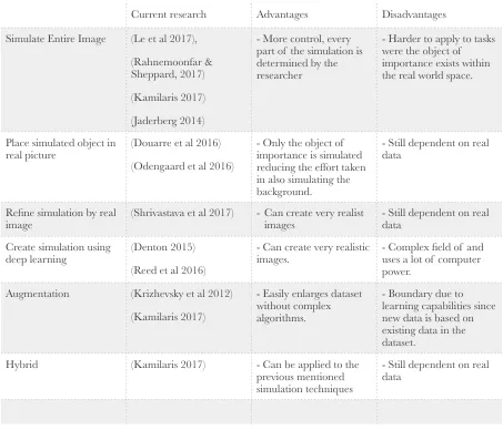
Table 1: Overview of simulation methods

Current research Advantages Disadvantages

Simulate Entire Image (Le et al 2017),

(Rahnemoonfar & Sheppard, 2017)

(Kamilaris 2017)

(Jaderberg 2014)

- More control, every part of the simulation is determined by the researcher

- Harder to apply to tasks were the object of importance exists within the real world space.

Place simulated object in

real picture (Douarre et al 2016) (Odengaard et al 2016)

- Only the object of importance is simulated reducing the effort taken in also simulating the background.

- Still dependent on real data

Refine simulation by real

image (Shrivastava et al 2017) - Can create very realist images - Still dependent on real data

Create simulation using

deep learning (Denton 2015) (Reed et al 2016)

- Can create very realistic

images. - Complex field of and uses a lot of computer power.

Augmentation (Krizhevsky et al 2012)

(Kamilaris 2017)

- Easily enlarges dataset without complex algorithms.

- Boundary due to learning capabilities since new data is based on existing data in the dataset.

Hybrid (Kamilaris 2017) - Can be applied to the previous mentioned simulation techniques

3. Ideation

This chapter will focus on the ideation phase of the project. The goal of the ideation phase is to acquire the relevant information related to a certain problem and to use this information to create something novel that is useful to the client. Rather than user interaction, the focus of this project lies on proving or disproving a hypothesis. To do so, the right software has to be created that can properly perform the experiments needed for the research as well as showing the output of the experiments. To achieve this, the following research question is formulated:

“What are the proper requirements for a set of programs that can simulate images and test the validity of these simulations when they are used to train deep neural networks to make predictions about real data?”

3.1. Client background and needs

This project was made together with Andreas Kamilaris. The goal of the end product should be evaluated with him and focus on his needs. Dr. Kamilaris is a researcher based in the University of Twente originally from Cyprus. Dr. Kamilaris has previously worked on the Internet of Things and Smart Buildings and is currently doing research in Big Data. Dr. Andreas has seen that data shortage can often be a problem when training neural networks. A solution he proposes is too use simulated data instead of real data. In order to test the validity of simulated training data, he proposed the project “simulated data in neural networks”. At the first meeting, the desired conduction of the research was discussed. He proposed to start with a scenario that is simple to implement and do more complicated tasks with there was extra time. During the first quartile of the project, the goal was to simulate smoke as a result of forest fires. The simulation of smoke is relatively simple since it is clearly distinguishable from things that are not smoke and since smoke does not have many complex features.

3.2. Ideation with the client

not smoke and since smoke does not have many complex features. Also, the classification of smoke can be useful in preventing future disasters. By embedding camera’s in large forests and assessing the imagery with the imagined deep neural network, smoke can be detected at an early stage of a forest fire and be dealt with at an early stage. By choosing smoke detection, not only an academic requirement is met but also a real-world requirement in which it can be directly beneficial to the people involved. If the smoke idea was realised in a short amount of time and extra time was available, a more complex scenario would be dealt with. The client proposed to work with a counting problem. Using deep neural networks for counting can be especially beneficial in cases where the counting has to be done over a large dataset. Having the counting be done by humans in such cases can be very time-consuming and prone to errors, not to mention it is a very mundane and unfulfilling task. After discussing with the client, it was agreed that a counting neural network has to be made that can count the number of houses from a satellite image. Houses, as seen from a satellite perspective, are relatively objects of low complexity. usually, a simple rectangle object will be enough to properly represent a house as seen from a satellite perspective. Also, the edges of the house make it easily detectable by a neural network since it is so distinctly different from its

background. The counting of houses also satisfies a real life need in cases of urban planning, for instance in slums in underdeveloped countries.

3.3. Tinkering Phase

time spent on learning the basics of image manipulation and creation. In order to successfully test the validity of the simulated images when training deep neural networks, one has to become familiar with some form of machine learning environment. For this project, the Keras environment was used. Keras is an open source neural network library writing with the Python programming langue. Information about Keras and how to use it was gathered from different sources found online ranging from video tutorials, articles and scientific papers. By using these sources of information, small applications were made that helped in gaining knowledge that was used to create the final product. One example in particular that helped a lot in gaining new knowledge was a tutorial on the development of an MNIST-digit predictor. The goal was to write a program using Keras that can successfully predict handwritten digits taken from the MNIST dataset. In the end, a program was written that was able to predict handwritten digits with a validation accuracy of 98%. The tutorial itself only focused in achieving a high validation accuracy but did not explain how to display the images together with the predicted output also it was only tested on images from the MNIST dataset and did not allow the user to create their own handwritten digit and feed it to the model to be tested. This was something that would be useful later on in the project when working with the simulated data. So the original program was modified to also implement this feature.

3.4. Requirements

Based on the clients needs the following requirements are set out for the the project. 1. A program has to be written to simulate images.

1.1. The images made using the program have to be of a certain level or realism in order to successfully use the images when training deep neural networks.

1.2. The program has to be written in Python and make use of some type of image creation/manipulation library.

1.3. The code has to be useable for other researchers, use clear semantics and stick to one type of coding convention.

1.4. The program does not require a user interface; it is assumed that the user is familiar with Python.

1.5. The program must be able to create multiple images with an amount specified by the user.

1.6. The program must be able to save these images to a specified folder on the users computer

2. The type of image has to be in an application domain where it has not been used before. 3. The type of image that is simulated has to be identifiable by itself.

4. The type of image that is simulated also has to be useful outside of the scope of artificial intelligence itself. For instance, relating to the environment, disaster prevention,

agriculture etc.

5. A deep neural network has to be created that can be trained on the simulated data and also validated on real data.

5.1. The neural network must be able to successfully learn from simulated data. 5.2. The neural network must be made using some deep learning environment 5.3. The neural network must be able to detect false positives and true positives and

display them to the user.

3.5. Conclusion

4. Realisation

This chapter describes the realisation phase of the the project. Each section focuses on a specific problem during the realisation phase and how this problem was solved. the conclusion can be found in the end of this chapter. The introduction provides a short overview of the overall process of the project. The conclusion describes how the requirements as shown in the ideation chapter are met.

4.1. overview

The goal of the research is to determine whether the use of simulated data as training data in deep neural networks is a reliable training method when working with image classification. To test its validity, the model was trained on real data as well as on simulated data. After the tests were performed, the validation accuracy when using real data is compared to the validation accuracy when using simulated data. At the beginning of the project, the aim was to create a simple scenario to test the validity of the use of simulated data. In order to create a simple scenario for image classification, the object in the images has to meet a few requirements. Firstly, the object has to be of a complexity that is low enough to be simulated using computer software. For instance, creating simulations of different breeds of dogs is a more difficult task than creating simulations of different types of fruit since the number of features is less in the second case. Secondly, the object has to be of a type that is easily detectable by a deep neural network. In order to meet these requirements, the first goal of the project was to simulate smoke as a result from large fires and test its validity as data source for deep neural networks. Smoke was chosen because it is easily simulated using computer software, also it has a distinct colour and shape that is easy to distinguish from its background. The simulations of smoke were made using the Pillow and the Perlin Noise libraries in python. After the simulations of smoke were made, they had to be used to train a deep neural network. In order to test the validity of the simulated data, the validation accuracy as a result of the use of simulated data had to be compared to that of the use of real data. Finally, a hybrid approach was also used which combines both real and simulated data in it’s learning process.

accuracy with very little computational power. It is one of the best pre-trained deep neural networks as of today.

When trying to train the models on a computer locally it quickly became apparent that the computer power was not sufficient enough for training these types of deep neural network. Instead of a local computer, a cloud computing service that possesses more computer power called Linode was used.

Applying the three different training types and the two different types of deep neural networks, six tests were run. After the tests were run it became apparent that the shallow model outperformed the pre-trained model. with a validation accuracy of 0.8, 0.9 and 0.9 for the simulated data, real data and hybrid data respectively. Here it seemed that although not perfect the use of real data was still superior to the use of simulated data. In order to improve the validation accuracy of the shallow model, two dropout layers were added. By adding the dropout layers, the validation accuracy for both the real, simulated and hybrid approach improved to a value of 1.0. meaning a perfect validation accuracy for each of the approaches.

4.2. Creating proper simulations of smoke

The first goal was to create simulations of smoke in Python using the Pillow library. It soon became clear that Pillow has it’s limitations when working with more complex image

generation. A crucial functionality, that was missing in Pillow, when making realistic smoke is Perlin-noise. Perlin-noise is a type of semi-random noise that is used in computer graphics to create realistic looking natural phenomena such as clouds, mountains, smoke etc. Since the Perlin-noise functionality is not part of Pillow, an extra library was used called Noise. Noise allows the user to create different types of Perlin-noise by specifying certain parameters. With the use of the Noise library, successful simulations of smoke were made. One problem, however, was that the simulated image only contains smoke without a background on which the smoke is displayed. In order to create a background, two options were evaluated. The first option was to create a background using image generation methods as done by

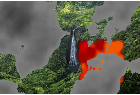
advantage of this approach is that the simulated picture is more like a real picture since the backgrounds are taken from actual foto’s. These backgrounds have a level of realism that can’t be achieved using simulation methods. See figure 1 for an example of the final result.

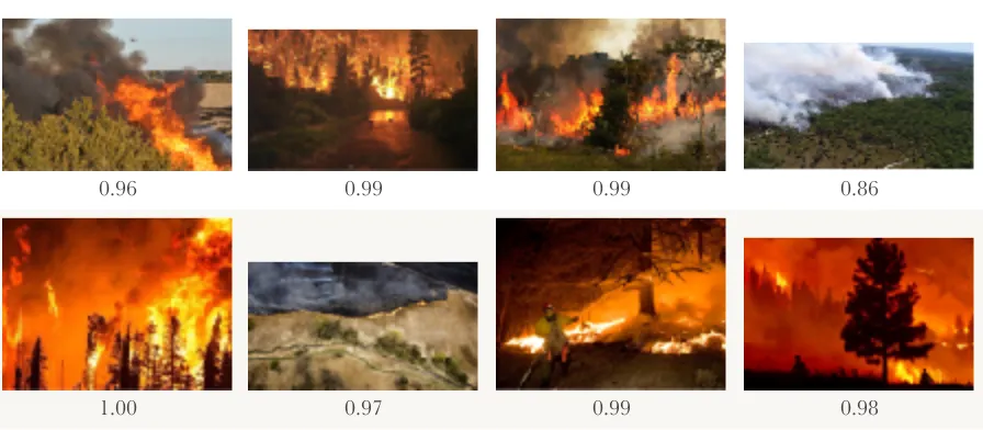
When using these images to train the neural network and detecting for false negatives (pictures that are classified as not containing smoke but actually do) it became apparent they had their shortcomings. Figure 2 shows the pictures of smoke that were wrongly classified as being pictures not that contain smoke..

Figure 2. False positives, smoke and fire

As can be seen by these pictures, most of the time pictures that contain a large portion of fire are wrongly classified as a picture that does not contain smoke. In order to prevent these false negatives from happening, the simulated images were modified to contain objects of varying shades of red and orange to represent fire. This was done by using the images of forests that were originally used to train the model on pictures that do not contain smoke. A set of circles of random size and varying shades of red and orange were created and lumped together at a random position on the image of a forest using the Pillow library. After this was done, every circle was given a gaussian blur to make the entire object more representative of fire and look less like a set of random circles. After the fire simulation was placed on the image, the smoke simulation that was previously used was layered on top of the fire simulation. Making it look as if the fire is coming from the forest shown in the image. Figure 3 shows an example of the final result.

False Positives - smoke and fire

!

0.96

!

0.99

!

0.99

!

0.98

!

0.99 ! 0.86

!

Figure 3. Synthetic smoke and fire with the background taken from real image

As can be seen from the picture above, a large portion of red material is added to represent fire. In must be noted that not every picture from the real image dataset contains a fire, most of the pictures in this dataset only contain smoke. It is because of this that the simulation program was modified to only simulate pictures containing fire a 30% of the time. When adding the simulated fire and testing for false positives, still a number of pictures that contain mostly fire show up. However, the pictures that only partly contain fire are no longer being detected as “not smoke”. See figure 4 for a view examples of false positives as a result from adding the synthetic fire.

4.3. Creating proper simulations for houses

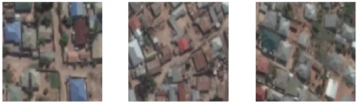
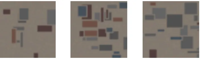
After the smoke simulations were made and tested, simulations of houses as if taken from satellite images were made. This was possible because, after the smoke phase, there was still time left to explore other areas of simulated data for deep learning. The initial idea was to test the simulations on drone images from the Open Tanzania Challenge from werobotics.org. However, after contacting them, no response was given. So instead, satellite images of slums in Tanzania taken from google earth were used. These images were later segmented into images of dimensions of 100x100 pixels. See figure 5 for a couple of examples of such an image.

Figure 5. Examples of validation images for the houses scenario

Dataset 1

Based on these images, the requirements for the simulated images were set. The simulated images need to have some have a background in some type of light brownish colour. Also, the images need to consist of multiple rectangle-like objects of different colours of blue, red and orange. Also, each house was given a border of 2 pixels similar to the colour of the

Figure 6. Examples of the images in the synthetic training dataset for dataset 1.

Dataset 2

As can be seen, by the images above, a lot of houses were created that were too small to be accurately predicted. This is a result of overlapping houses and their borders. After this was noticed, a new program was written that prevents the houses from overlapping and thus also prevent houses that are too small from being generated. The new program segmented each image into 25 segments as follows:

Depending on the number of houses in the image, each segment was filled with either one house of random size and location or no house at all. This prevents the houses from

overlapping and creates an evened out image. See figure 8 for a couple of examples of such an image.

Figure 8. Examples of the images used in the synthetic training dataset for dataset 2.

4.4. Implementing the code in Jupyter

When working with deep neural networks, running the code can often be time-consuming because of the large amount of time needed to properly train a neural network. Jupyter allows the user to run different sections of the code by using a graphical user interface run on a web browser. This way the code segment used from training the neural network can be run separately from other code segments, reducing the time needed for debugging when other code segments are not working properly. Also, Jupyter allows the user to display graphical outputs relating to each individual code segment creating a more organised and structured work environment and as a result improving the workflow. Because of these advantages, the client requested to use Jupyter.

4.5. Running the code on a cloud platform

option was to run the code on a cloud that employs superior computing power. This would be preferable to the first option since the services of the cloud are available at all times. At first, the Google cloud platform was looked into. However, it quickly became apparent that this was not the right platform for the research since it requires the user to use the interface provided by Google making it overly complex and limiting the user's freedom. A second option which was more reliable was to use the cloud platform provided by Linode. Linode is a virtual private server that allows the user to run several Linux distributions. The advantage of this is that the user can work on a familiar operating system and install the right packages and libraries like one would do on a local Linux distribution by using the terminal. The chosen operating system was Ubuntu 16.04. Ubuntu is a widely used Linux distribution backed by a large community ready to answer questions when running into different types of problems. It must be noted that when running an operating system on Linode, no graphical user interface is given. This means that every operation like for instance copying files, installing libraries, editing files, etc has to be done via the terminal. One disadvantage of the absence of a graphical user interface is the absence of a web browser used for Jupyter. Unfortunately, this deprives the research of the usability of an environment such as Jupyter. Because it was impossible to run Jupyter on the Linode server, python files were used when running the codes on the server. The following list provides an overview of the specifications of the Linode instance used in the research:

- RAM: 8GB - Cores: 4 CPU’s - Storage: 160 GB SSD - Transfer 5TB

- Network in: 40 Gbps - Network out: 5000 Mbps

- Operating system: Ubuntu 16.04 64bit

4.6. Making accurate predictions based on simulated data for

smoke

‘Smoke’ and ‘Forest’ containing their representative images. The validation metrics used in this case was accuracy. The accuracy calculates the percentage of data points (in this case images) that were properly predicted. For instance, if out of a set of hundred images, eighty were properly predicted, the validation accuracy would be 0.8.

The first thing to consider is whether the use of simulated data is superior to the use of real data in regards to validation accuracy. This is done by comparing the validation accuracy of the simulated data scenario and to the validation accuracy of the real data scenario. This results in two approaches; the real data approach in which real data is used and the simulated approach in which simulated data is used. Additionally, a hybrid approach was proposed in which both real and simulated data were used. The second thing to consider is which type of model is best suited for training the deep neural network model. Two types of models were used; a shallow model and a pre-trained model. Bellow is an explanation of each of these two models. Bellow is an explanation for each of the different approaches as well as the types of models that were used.

Real data approach:

The training data consisted only of real data. The folder named ‘Smoke’ consisted of pictures taken from the internet that contain smoke as a result from some form of disaster or forest fire. The folder named ‘Forest’ contained pictures of forest taken from a helicopter

perspective.

The validation folder also consisted of pictures that contain either smoke or forest. Although the images in the validation folder were of the same type as the images in the training folder, it is very important that not exactly the same pictures as from the training folder are used in the validation folder and vice versa.

Simulated data approach:

The training data consisted of both real and simulated data. The folder named ‘Smoke’ consisted of simulated images as shown in section 1 of this chapter. The folder named ‘Forest’ consisted of the same images that were used in the testing on real data scenario.

Hybrid approach:

The model was first trained using only real data. The weights from the model were saved and later retrained on simulated data to achieve a higher validation accuracy.

Shallow model:

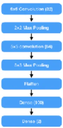
A shallow model is a type of model used in neural networks that have a small number of hidden layers. The advantage of shallow networks is that they take less time when training. The disadvantage of shallow networks is that it is less suited for more complicated tasks. For instance, images that contain a lot of complex and different features. The following diagram represents the architecture of the shallow model that was used:

Figure 9. The architecture of the shallow model that was used.

Pre-trained model:

As the name suggests, a pre-trained model has already been heavily trained on a large data set. In this case, the pre-trained model was trained using the ImageNet data set. By training on this data set, the model is able to detect a wide range of images. It is however not able to detect images that fall outside the ImageNet dataset. This is where re-training comes into play. During the training process, a pre-trained model called InceptionV3 was used.

Figure 10. Graph of the current pre-trained models located on the graph in regard to the number of operations (x) and the top-1 accuracy in percentage (y)

In the ideation chapter of this report, several requirements are laid out that have to be

- Real data was used to train a shallow model - Simulated data was used to train a shallow model

- A hybrid of real and simulated data was used to train a shallow model - Real data was used to train a pre-trained model

- Simulated data was used to train a pre-trained model

- A hybrid of real and simulated data was used to train a pre-trained model

4.7. Making accurate predictions based on simulated data for

houses

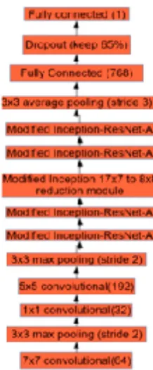
In order to test the validity of the simulated images a model based on the model used by Rahnemoonfar & Sheppard (2017) was used. In their research on using simulated data to count the amounts of tomatoes in a tomato plant, a deep convolutional neural network was used with several modified ResNet-50 layers. The overall architecture of the model used in this study looked as follows:

The Modified Inception-ResNet-A layers, as well as the modified Inception layer, were altered to look as follows:

Figure 12. Modified inception ResNet-A layer.

formulated as follows, with n being the amount of data points, Y being the predicted value and Ŷ being the actual value:

!

Figure 13. The formula for calculating the Mean Squared Error.

For each training session, the model was slightly modified to find the model with the lowest mean squared error. Also, for each training session, the weights of the epoch that resulted in the lowest mean squared error were saved. Figure 14 shows each modification A, B, and C of the model as shown in figure 11.

Figure 14. The three modifications (A, B and C) made on the model designed by Rahnemoonfar & Sheppard as depicted in figure 11.

MSE

= 1

_n

_∑

n

i

=1

Also, the drop out layer was changed from 65% to 10% drop out for each of the three models. The validation metrics used in this case was mean squared error since the model was dealing with a regression problem instead of a classification problem as was the case in the smoke vs forest scenario. In total the following six different types of models were trained and later validated.

5. Results

5.1. Smoke VS Forest

For the smoke VS forest scenario, two types of models were used, each with three types of data, in the end, six scenario’s were tested. The following graphs show the testing results over multiple epochs. For each training session, the best epoch was saved.

Figure 15. Graphs of the validation accuracy and training accuracy of the shallow model as a result of training the model on real (A), synthetic (B) and hybrid data (C).

(B) Accuracy of the model trained on synthetic data.

0,5 0,6 0,7 0,8 0,9 1

1 2 3 4 5 6 7 8 9 10

(C) accuracy of the model trained on hybrid data.

0,5 0,6 0,7 0,8 0,9 1

1 2 3 4 5

(A) Accuracy of the model trained on real data.

0,5 0,6 0,7 0,8 0,9 1

Figure 16. Graphs of the validation accuracy and training accuracy of the pre-trained model as a result of training the model on real (A), synthetic (B) and hybrid data (C).


(A) Accuracy of the model trained on real data

0,5 0,6 0,7 0,8 0,9 1

1 1 2 3

(B) Accuracy of the model trained on synthetic data

0,5 0,6 0,7 0,8 0,9 1

1 1 2 3

(C) Accuracy of the model trained on hybrid data

0,5 0,6 0,7 0,8 0,9 1

After the previous six scenario’s, two dropout layers of 10% were added to the shallow model. the following graphs show the testing results over multiple epochs

Figure 17. Graphs of the validation accuracy and training accuracy of the shallow model with 10% dropout as a result of training the model on

real (A), synthetic (B) and hybrid data (C).

0,5 0,6 0,7 0,8 0,9 1

1 3 5 7 9 11 13 15 17 19 Validation Accuracy - Real - 10% dropout Training Accuracy - Real

0,5 0,6 0,7 0,8 0,9 1

1 3 5 7 9 11 13 15 17 19 Validation Accuracy - Sim - 10% dropout Training Accuracy - Sim

0,5 0,6 0,7 0,8 0,9 1

1 2 3 4 5 6 7 8 9 10

For each epoch of each model, the weights of the best epoch were saved. The validation accuracies can be seen in table 1 and table 2 As can be seen in Table 1, By using a shallow model trained on real data, a validation accuracy of 0.9 can be reached. And when using a shallow network trained on simulated data, a validation accuracy of 0.8 can be reached. Also, the shallow network outperforms the Inception V3 network for each type of data it was trained on. When adding a dropout of 10%, the model can reach a validation accuracy of 1 for each type of data used.

Table 1: Best validation accuracy for each method - no dropout.

Shallow Inception V3

Simulated data 0.8000 0.62

Real Data 0.9000 0.69

Hybrid 0.9000 0.71

Table 2: Best validation accuracy for each method - with 10% dropout.

Shallow

Simulated data 1.0000

Real Data 1.0000

5.2. Houses

For the houses scenario, two types of synthetic data were used as described in chapter 4.3. Both types of synthetic data were used to train the three types of models as shown in figure 14, each model was tested with 65% dropout and 10% dropout, in the end, twelve scenario’s were tested. In order to test the reliability of the simulated training data as well as the models, the models were validated on both real and simulated data. The metrics for validation was the mean squared error. Each training session was done over 10 epochs.

Model trained on synthetic data and validated on real data when using dataset 1:

At first, dataset 1 was used as shown in chapter 4.3. The validation mean squared error more or less stayed the same and showed little fluctuations after the first epoch. The following table shows the lowest validation mean squared error for each scenario tested when using real data in the validation set.

When testing the reliability of the predictions the model with the lowest mean squared error was tested, which in this case was model c with 65% dropout. In order to accurately interpret the results of the model, a couple of data points have to be tested and evaluated. In this case, the validation images were also used as testing images. The following list shows the predicted output of the first nine validation images as well as the actual value:

Table 3: Lowest mean squared error for each model using 65% dropout or 10% dropout. Validated on real data

65% dropout 10% dropout

Model A 43.33 43.01

Model B 42.92 41.93

1: predicted: 8.70288467407 actual: 32 2: predicted: 8.57694149017 actual: 20 3: predicted: 8.58588504791 actual: 10 4: predicted: 8.64188098907 actual: 17 5: predicted: 8.63617610931 actual: 10 6: predicted: 8.60346412659 actual: 19 7: predicted: 8.61840629578 actual: 17 8: predicted: 8.6007976532 actual: 16 9: predicted: 8.68910503387 actual: 7

As can be seen by this list, al validation images are predicted to contain a quantity of houses around 8.6, independent on the actual data. This means that the model was not able to accurately predict the number of houses located in each picture.

Model trained and validated on synthetic data when using dataset 1:

As can be seen by the predictions on the model that is validated on real data, the output is not reliable. In order to investigate the issue and see if the problem lies in the validation data, the model was trained on synthetic data and also validated on synthetic data. The validation mean squared error more or less stayed the same and showed little fluctuations after the first epoch. The following table shows the lowest validation mean squared error for each scenario tested when using real data as the validation set.

Table 4: Lowest mean squared error for each model using 65% dropout or 10% dropout. Validated on synthetic data

65% dropout 10% dropout

Model A 23.36 23.42

Model B 22.34 21.93

When testing the reliability of the predictions the model with the lowest mean squared error was tested, which in this case was model c with 65% dropout. In order to accurately interpret the results of the model, a couple of data points have to be tested and evaluated. In this case, the validation images were also used as testing images. The following list shows the predicted output of the first nine validation images as well as the actual value:

1: predicted: 7.21706771851 actual: 22 2: predicted: 7.1572303772 actual: 16 3: predicted: 7.16448640823 actual: 13 4: predicted: 7.18330430984 actual: 20 5: predicted: 7.18099308014 actual: 24 6: predicted: 7.17154598236 actual: 10 7: predicted: 7.1847615242 actual: 20 8: predicted: 7.17476129532 actual: 16 9: predicted: 7.21042251587 actual: 15

As can be seen by this list, the same problem arises as was the case when validating on real data. Al validation images are predicted to contain a quantity of houses around 7.1,

independent on the actual data. This means that the model was not able to accurately predict the number of houses located in each picture.

Results when using dataset 2

As can be seen in the previous table, no improvements were made using dataset 2, in fact the results got worse. It is for this reason that the model was not tested to make predictions about individual images as done for dataset 1.


Table 5: Lowest mean squared error for each model using 65% dropout or 10% dropout. Validated on real data

65% dropout 10% dropout

Model A 45.84 44.06

Model B 44.47 44.37

Training and validating the model with simple counting data

As can be seen by the results of dataset 1 and dataset 2, either the data is not a reliable source for training deep learning models or the wrong type of model is used. To test the validity of the model, the model was trained on a dataset of pictures that contain a multitude of dots of colours red, blue and green. Figure 18 shows an example of such an image.

Figure 18. Example of an image taken from the simple dataset.

The advantage of this dataset is that the type of images of the dataset are very simple and have low complexity. Also, the dataset contains 42500 images for the training dataset and 7500 images for the validation dataset, which is a large number of images and should thus improve the reliability of the model when trained on this dataset. Because of the simplicity of the images and the large number of images that are in this dataset, it is a very reliable source for testing the validity of the model. If the model is trained on this dataset and still shows a mean squared error that is too high, the problem most likely has to do with the model itself. Having this knowledge will be helpful in future research. The model was trained to count the amount of red dots that were located in each picture. By using model c with a 65% dropout a validation mean squared error of 3.67 was reached. This might seem like an improvement to the validation mean squared error of the previously used cases with dataset 1 and dataset 2. However, it must be noted that the maximum dots of one colour per image is five. A

Finally, a classification model was used instead of a regression model and the metrics used was validation accuracy instead of validation mean squared error. By using this new type of model a validation accuracy of 0.985 was reached. This shows that sometimes a counting task can be seen as a classification problem instead of a regression problem. The following figure shows a few examples of the predictions of the classification model:

actual: 4 - predicted: 4 actual: 3 - predicted: 3 actual: 3 - predicted: 3

Figure 19. Actual values and predictions of the classification model trained on simple data

To see whether this method also applies to the counting of houses, the same model was used, using dataset 2 as both the training and the validation data. A validation accuracy of 0.4225 is reached. The model was also tested on the validation data, the following image shows a few examples of the predictions of the classification model:

actual: 15 - predicted: 22 actual: 22 - predicted: 16 actual: 6 - predicted: 13

6. Conclusion and future work

6.1. Smoke VS Forest

As can be seen by the results, the shallow model outperforms the inception V3 model for each of the three types of data used. This is most likely because the Inception V3 model was to complex for the given task and a more simple model might be more sufficient when the task is also more simple. By using simulated data, the model reached a validation accuracy of 0.8. This proves that synthetic data can be sufficient when training deep learning models. By adding a dropout of 10%, the model reached a validation accuracy of 1 when trained on synthetic data as well as when trained on real data.

When training the shallow model a validation accuracy of 0.8 is reached for synthetic data without dropout and a validation accuracy of 1.0 with 10% dropout. These results are very promising. However, one has to be aware that due to the scarcity of real data the value of the validation accuracy might be susceptible to chance and that this high validation accuracy is partly the result from a model that is guessing the right classification. In order to get a more reliable value for the validation accuracy, more data is needed for the validation dataset. Looking at the false positives, it becomes clear that the model is unable to classify pictures containing mostly fire as ‘smoke or fire’. This is the case for both synthetic and real data. By adding in blobs of synthetic fire the false positives were partly resolved. However, some validation images that contained mostly fire were still wrongly classified as ‘forest’. This is most likely because these images consisted of hardly any smoke and only consisted of fire. See figure 21 for such an image.

As can be seen by this picture it hardly consists of any smoke that is similar to the smoke created in the synthetic data set. In order to make better classifications in the future, the synthetic dataset has to be improved by adding larger simulations of fire and smaller simulations of smoke on top of the data already generated in this research.

In conclusion, when using synthetic data, the model can reach a validation accuracy as high as with synthetic data. However, this could just be a case of the model guessing the right answer. In further research, using a larger more varied dataset is advised. Also, the synthetic training dataset could be improved by adding more pictures that represent the pictures in the validation dataset such as pictures that mostly or only contain fire.

6.2. Houses scenario

As can be seen by the results the model performs best with just one modified inception resent layer and a dropout of 65% for both types of simulation. The best epoch of the model using synthetic dataset 1 had a validation mean squared error of 41.65 when validated on real data and a validation mean squared error of 21.54 when validated on synthetic data.

Unfortunately, this is a higher mean squared error than was originally intended. When training the model on synthetic dataset 2, the model was able to reach a validation mean squared error of 43.75 when validated on real data.

houses would belong to the class ‘five’, an image of six houses to ‘six’, etc. When treating the task as a classification problem for the simple dataset, a validation accuracy of 0.985 was reached. This shows that treating counting tasks as a classification problem might be

References

Oates, T., & Jensen, D. D. (1998, August). Large Datasets Lead to Overly Complex Models: An Explanation and a Solution. In KDD (pp. 294-298).

Garcia, J., Barbedo, A. (2018). Impact of dataset size and variety on the effectiveness of deep learning and transfer learning for plant disease classification. Computers and Electronics in Agriculture (pp. 46-53).

Cho, J., Lee, K., Shin, E., Choy, G., & Do, S. (2015). How much data is needed to train a medical image deep learning system to achieve necessary high accuracy?

Too, E. C., Yujian, L., Njuki, S., & Yingchun, L. (2018). A comparative study of fine-tuning deep learning models for plant disease identification. Computers and Electronics in Agriculture.

Fakoor, R., Ladhak, F., Nazi, A., & Huber, M. (2013, June). Using deep learning to enhance cancer diagnosis and classification. In Proceedings of the International Conference on Machine

Learning (Vol. 28). New York, USA: ACM.

Cios, K. J., & Moore, G. W. (2002). Uniqueness of medical data mining. Artificial intelligence in medicine, 26(1-2), 1-24.

Dai, S. (2018) AI promises jobs revolution but first it needs old-fashioned manual labour – from China. South China Morning Post.

Schmidhuber, J. (2015). Deep learning in neural networks: An overview. Neural networks, 61, 85-117.

Cireşan, D., Meier, U., & Schmidhuber, J. (2012). Multi-column deep neural networks for image classification. arXiv preprint arXiv:1202.2745.

Jaderberg, M., Simonyan, K., Vedaldi, A., & Zisserman, A. (2014). Synthetic Data and Artificial Neural Networks for Natural Scene Text Recognition.

Odengaard, N., Knapskog, A. O., Cochin, C., & Louvigne, J. C. (2016) Classification of ships using real and simulated data in a convolutional neural network.

Rahnemoonfar, M., & Sheppard, C. (2017). Deep count: fruit counting based on deep simulated learning. Sensors, 17(4), 905.

Le, T. A., Baydin, A. G., Zinkov, R., & Wood, F. (2017). Using synthetic data to train neural networks is model-based reasoning. In Neural Networks (IJCNN), 2017 International Joint

Conference on (pp. 3514-3521). IEEE.

Mhaskar, H., Liao, Q., & Poggio, T. A. (2017). When and why are deep networks better than shallow ones?. In AAAI(pp. 2343-2349).

Goodfellow, I., Pouget-Abadie, J., Mirza, M., Xu, B., Warde-Farley, D., Ozair, S., ... & Bengio, Y. (2014). Generative adversarial nets. In Advances in neural information processing systems (pp. 2672-2680).

Shrivastava, A., Pfister, T., Tuzel, O., Susskind, J., Wang, W., & Webb, R. (2017, July). Learning from Simulated and Unsupervised Images through Adversarial Training. In CVPR(Vol. 2, No. 4, p. 5).

A. Kamilaris, A. Kartakoullis and F. X. Prenafeta-Boldú. A Review on the Practice of Big Data Analysis in Agriculture. Computers and Electronics in Agriculture International Journal, 143(1): 23-37, 2017.

Kamilaris, A. (2017). Simulating Training Data for Deep Learning Models. Presented at EnviroInfo 2018.

DOUARRE, C., SCHIELEIN, R., FRINDEL, C., GERTH, S., & ROUSSEAU, D. (2016). Deep learning based root-soil segmentation from X-ray tomography. bioRxiv, 071662.

Bousmalis, K., Irpan, A., Wohlhart, P., Bai, Y., Kelcey, M., Kalakrishnan, M., ... & Levine, S. (2018, May). Using simulation and domain adaptation to improve efficiency of deep robotic grasping. In 2018 IEEE International Conference on Robotics and Automation (ICRA) (pp. 4243-4250). IEEE.