ECE-520 Lab 8
Full Order (Prediction) Observers with State Variable Feedback and Integral
Control For One and Two Degree of Freedom Systems using Different Sampling
Rates
Overview
In this lab you will be repeating the procedures you utilized in Lab 7, but this time we will be examining the effects of reducing the sampling time. In some ways the system will work better for reduced sampling times, but it does become more difficult as the time interval becomes small.
For each of the systems you use in this lab you will go through the following basic procedure:
1) You should modify your Matlab code to be able to change the sampling rates. The pieces of code necessary to do this are on the class webpage. Be sure you load the appropriate continuous time model (from labs one or two) before you sample.
2) You should try sampling with at least three different sampling intervals, separated by 0.01 (that is, don’t sample at intervals of 0.05, 0.051, 0.052…Try things like 0.06, 0.04, 0.035 etc.). It will be probably be difficult with sampling intervals near 0.01.
3) Simulate the system to determine if your model meets the desired specifications. If it does not, modify the pole locations until it does meet the specifications. In addition, you need to be sure the control effort does not reach the saturation level. The simulated control effort for the discrete-time system does not model the real control effort as well as it does for the continuous time system.
4) Once you have simulated the system all of the variables you used are in Matlab’s workspace. Now compile the correct ECP driver file that replaces the model of the ECP system with the ECP system driver (and the real ECP system). Reset the ECP system, and run the system.
Notes and Guidlines:
• Although it should not matter, only use positive pole locations. Apparently the ECP systems are not particularly happy with negative pole locations.
• We are going to have to have to poles fairly close to the origin for our systems to work. However, as the sampling rate increases, we will have to move the state feedback poles farther away. The observer poles should generally be closer in than the state feedback poles.
• The ECP systems really do not like poles at the origin, so don’t put any state feedback poles there (no deadbeat control.) However, for many of your systems you should be able to put the observer poles there.
• Run the systems for at least one second, but don’t run the system so long most of your graph shows the system at steady state.
• Reset the system each time before you run it.
• As soon as you start you controller (click on play) be prepared to stop the system. In particular, listen for vibrations that are growing louder and stop the system as soon as possible after this.
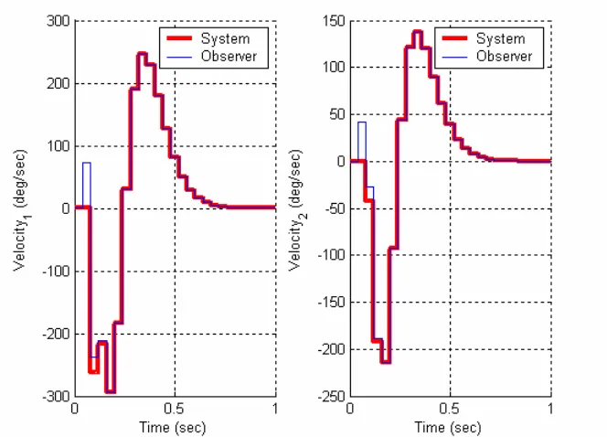
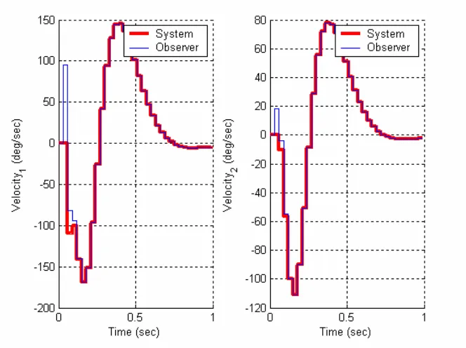
Figures 1-5 show typical behavior you should be aware of. In Figure 1, there is a nice smooth transition in the velocities. The system might actually be able to move like this. In system 2, at a higher sampling rate, there are some notches in the velocity. Our systems probably can’t match this exactly, but they will probably do ok. In Figure 3, at a higher still sampling rate, the
Figure 1: ``Acceptable’’ velocity plots. This might actually work (Ts = 0.5, feedback poles all at 0.4)
[image:3.612.141.473.419.658.2]Figure 3: Sampling interval is Ts = 0.3. Our systems will not be able to match the velocity, particularly for the first cart. All poles still at 0.4.
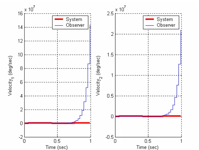
[image:4.612.140.472.398.646.2].
Figure 5: Sampling interval is Ts = 0.3. All poles have been moved out to 0.8. Our system will try and match this, but it won’t be pleasant.
Design Specifications
For each of your systems try and have the simulated systems meet the following design specifications
a) Settling time less than or equal to one second
b) Steady state error is zero for a 1 cm step input (or a 15 degree step input) c) Percent overshoot less than 20%
You should try for the 1cm (or 15 degree) inputs, but if your system is unwilling to cooperate try a 0.5 cm input (or a 10 degree input). This is particularly true when trying to control the position of the second cart/disk.
Note that the error in the observers will really only go to zero if the model exactly matches the real plant. This is not the case for us, so you can expect the estimated states to differ from the real states, particularly the states which are velocities.
Part A1: One Degree of Freedom Rectiliner Systems without Integral Control
7. However, if you used a model derived from the system identification toolbox it may not match that well.
b) Set all initial conditions in your simulation to zero.
c) Run the simulation for at least one second (Tf should be at least one second). This is because the ECP systems tend to hang up if they run for less than a second.
d) Simulate the system, check to see that they meet the design requirements and the control effort does not reach the saturatation level. If there is a problem try a different set of pole locations.
e) Reset the ECP system.
f) Connect Model210_DT_sv1_observer.mdl to the ECP system and run it.
g) Plot the measured and estimated states on the same graph. Do not plot the third state since it is not really all that important.
h) Copy and paste this graph into your Word document that will eventually become your memo for this lab. It is a real good idea to write a short caption at this time so you don’t forget what you just did.Be sure to include the (observer and state feedback) pole locations in the caption. In addition, include the sampling interval.
i) Repeat this procedure for two additional sampling intervals (different than 0.05)
Part A2: One Degree of Freedom Rectiliner Systems with Integral Control
For this part do the same thing you did in part A1, except utilize integral control. Be sure to include the (observer and state feedback) pole locations, and the sampling intervals, in the caption.
Part B1: Two Degree of Freedom Rectiliner Systems without Integral Control
For this system you need to basically go through the same steps you used in PART A1
Assume the observer has available the position of the second cart. If this does not work very well assume it has available the positions of both carts. We are trying to control the position of the first cart, and then we are trying to control the position of the second cart. (Two separate cases.) You should compare the estimated states with the real states for each of the two cases. Be sure to include the (observer and state feedback) pole location sand the sampling intervals in the caption.
Part B2: Two Degree of Freedom Rectiliner Systems with Integral Control
Similar to B1, but include the use of integral control.
Part C1: One Degree of Freedom Torsional Systems without Integral Control
For this system you need to basically go through the same steps you used in PART A1, except you will need to use the one degree of freedom torsional system.
Be sure to include a plot comparing the true and estimated states and include the pole locations. It should also indicate the sampling intervals. You should plot your outputs in degrees or degrees/second
Part C2: One Degree of Freedom Torsional Systems with Integral Control
Same as C1, but include integral control.
Part D1: Two Degree of Freedom Torsional Systems without Integral Control
For this system you need to basically go through the same steps you used in part B1, using the two degree of freedom torsional system.
Even though I indicated the desired input in degrees, your mathematical model (and the ECP system) works in radians, so your input must be in radians.
Be sure to include a plot comparing the true and estimated states and include the pole locations, as well as the sampling intervals. You should plot your outputs in degrees or degrees/second
Part D2: Two Degree of Freedom Torsional Systems with Integral Control
Same as D1, but include integral control.
Even though I indicated the desired input in degrees, your mathematical model (and the ECP system) works in radians, so your input must be in radians.
Be sure to include a plot comparing the true and estimated states and include the pole locations, as well as the sampling intervals. You should plot your outputs in degrees or degrees/second
Your memo should summarize how well the estimators predicted the true states of the systems, and whether including the integrator improved on the steady state error (compared to not having an integrator in the system). Was it easier to estimate the positions or the velocities? Did
sampling at higher rates (Ts smaller) improve the performance?
You should have a whole bunch of plots (A1-3, A2-3, B1-6, B2-6, C1-3, C2-3, D1-6, D2-6) and each caption should indicate the position of the state feedback and observer poles, as well as the sampling intervals.