External shocks

Munich Personal RePEc Archive

External shocks

Goyal, Ashima

Indira Gandhi Institute of Development Research

2014

Online at

https://mpra.ub.uni-muenchen.de/72498/

1

Preprint from Mahendra Dev (ed.) India Development Report, IGIDR and OUP, New Delhi, 2014

External shocks

Ashima Goyal*

Professor

Indira Gandhi Institute of Development Research Gen. Vaidya Marg, Santosh Nagar,

Goregaon (E), Mumbai-400 065 Tel.: (022) 28416512, Fax: (022) 28402752

[email protected]

http://www.igidr.ac.in/faculty/ashima

Abstract

After the global financial crisis, India was exposed to many external shocks from commodity prices and foreign capital flows. Although capital flow fluctuations were largely due to global risk-on risk-off factors, a widening current account deficit (CAD) contributed to India’s vulnerability to external shocks. The major source of shocks was external, but policy

mistakes increased India’s vulnerability. These included inadequate attention to sectoral bottlenecks that reduced export growth and domestic financial savings, while substitution away from expensive oil imports was discouraged. Dependence on foreign capital, to finance the CAD, rose while degrees of freedom from continuing capital controls were underutilized to reduce exchange rate volatility and to smooth interest rates. Steep depreciations combined with volatility did not help exporters. Evaluation of measures to stabilize the exchange rate establishes that temporarily taking oil marketing companies demand out of the market was the most effective, since small demand-supply mismatches lead to large currency movements in thin markets. Prudential measures such as increasing position limits, margin requirements are to be preferred to a ban on a market or a transaction-type. If market restrictions become necessary, they should be carefully targeted. Accumulation and use of reserves, use of market information and of signalling can all help implement managed floating. Such an exchange rate regime can contribute to effective inflation targeting without the policy rate rising to reduce depreciation as in the classic interest rate defense.

Keywords: External shocks; current account deficit; exchange rate regime; volatility; market interventions

JEL Codes: F41, F42, F31, F32, F36

*

2

1. Introduction

India experienced many external shocks from commodity prices and foreign capital flows in the post global financial crisis (GFC) period. Inelastic oil imports and inflation-driven demand for gold contributed to a widening of the current account deficit (CAD), and its financing became an issue. But fluctuations in capital flows largely follow global risk factors unrelated to domestic needs. Just talk of quantitative easing (QE) withdrawal (known as the taper on) lead to steep depreciation and loss of emerging market (EM) asset values in May 2013. March 2014 saw a reversal of sentiment with 30 EMs receiving USD 39 billion

compared to only 5 billion in January, according to the Institute for International Finance. But a surge normally ends in a sudden stop. The worst case for India is if oil shocks and global

risk-off, or rising risk aversion, occur together. This happened in late 2011 with the Euro debt crisis.

While advanced economies (AEs) recognize the collateral damage to EMs they tend to dismiss it saying EMs gained from inflows in the past, and will gain from AE revival; there is probably a bubble in EM assets that needs to burst. But if there is a bubble then how did EMs gain from QE induced inflows in the first place? QE hurt EMs by firming commodity prices and widening CADs. Easier inflow based finance allowed neglect of structural reforms, while encouraging over-stimulus. Inflows also first-over-appreciated EM currencies, then led to sharp depreciations. The Brazilian finance minister coined the term ‘currency wars’ for these gyrations. This chapter explores how India negotiated these global gales1.

The major source of shocks was external, but policy mistakes increased India’s vulnerability.

These included inadequate attention to removing domestic bottlenecks that reduced export growth, and domestic financial savings, while expensive oil imports rose. Dependence on foreign capital, to finance the CAD, was allowed to rise while degrees of freedom from continuing capital controls were underutilized to reduce exchange rate volatility and to smooth interest rates. High exchange rate volatility and steep depreciations did not help

exporters or industry.

The chapter examines aspects of openness, and shows despite twin deficits there was no generalized excess demand. Sectoral bottlenecks, oil shocks, and capital outflow associated

1

3

sharp depreciations widened the CAD. Evaluation of measures to stabilize the exchange rate establishes that temporarily taking oil marketing companies demand out of the market was the most effective, since small demand-supply mismatches lead to large currency movements in thin markets. The experience suggests managed floating can be achieved through measures such as accumulation and use of reserves, use of market information and of signaling. Such an exchange rate regime can contribute to effective inflation targeting without the policy rate rising to reduce depreciation as in the classic interest rate defense.

Various market restrictive measures reduced market turnover sharply in the currency derivatives markets in exchanges, while total turnover including the dominant

over-the-counter trading in banks also fell. This suggests the two types of markets are complements rather than substitutes. Offshore markets grew at the expense of domestic markets. Therefore prudential measures such as increasing position limits, margin requirements are to be

preferred to a ban on a market or a transaction-type. If market restrictions become necessary, they should be carefully targeted. Since administrative measures can reduce one-way

positions, a general liquidity squeeze such as an interest rate defense, should be avoided. When the latter was attempted in mid-2013, an inadequate rise in short-term rates raised already high interest rate spreads and long-term rates, hurting the domestic recovery and domestic financial markets.

The remainder of the chapter is structured as follows: after section 2 sets out the degree of openness and analyzes the effects of shocks, section 3 examines determinants of the CAD. Section 4 brings out the policy failures that compounded external shocks. Section 5 draws out lessons on what measures proved to be most effective in reducing the impact of external shocks on the exchange rate, and their effect on foreign exchange (FX) markets. This leads on to the discussion of the exchange rate regime in the context of inflation targeting in section 6, before section 7 gives some pointers for the way forward for domestic and international policies.

2. The degree of openness

4

Figure 1: India's balance of payments (ratio to GDP)

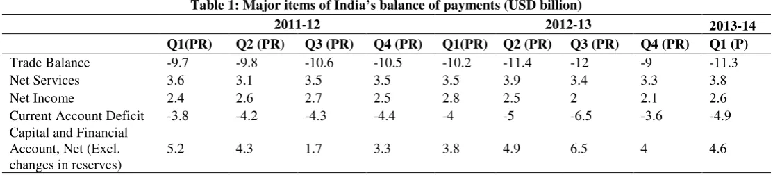
Table 1: Major items of India’s balance of payments (USD billion)

2011-12 2012-13 2013-14

Q1(PR) Q2 (PR) Q3 (PR) Q4 (PR) Q1(PR) Q2 (PR) Q3 (PR) Q4 (PR) Q1 (P)

Trade Balance -9.7 -9.8 -10.6 -10.5 -10.2 -11.4 -12 -9 -11.3

Net Services 3.6 3.1 3.5 3.5 3.5 3.9 3.4 3.3 3.8

Net Income 2.4 2.6 2.7 2.5 2.8 2.5 2 2.1 2.6

Current Account Deficit -3.8 -4.2 -4.3 -4.4 -4 -5 -6.5 -3.6 -4.9

Capital and Financial Account, Net (Excl. changes in reserves)

5.2 4.3 1.7 3.3 3.8 4.9 6.5 4 4.6

Note: Total of subcomponents may not tally with aggregate due to rounding off. PR: Partially Revised. P: Preliminary. Source: RBI Macroeconomic and Monetary Developments various years

Figure 1 shows there was a CAD in most years. Since this is exports minus imports of goods and services, it takes a negative value. It was however relatively stable in the post reform period, varying between -3 and +2.3 as a ratio of GDP, until after the GFC when it first fell below -3, which is widely regarded as the sustainable level. It even reached -6.5 percent in Q3 2012-13 (Table 1). The deficit was much larger on the trade account, but was partially compensated by a surplus on invisible items such as net services.

A deficit requires foreign capital to finance it. This was not a problem in the pre GFC years as capital inflows rose sharply and the deficit was moderate. The capital account peaked at 9.2 as a ratio of GDP in 2007-08, although there were fluctuations. Figure 1, which graphs components of the BOP as a percentage of GDP, shows the change in reserves to be a mirror image of the capital account—peak capital flows were largely absorbed in reserves, since they much exceeded the CAD.

-10 -5 0 5 10 19 90-91 19 91-92 19 92-93 19 93-94 19 94-95 19 95-96 19 96-97 19 97-98 19 98-99 19 99-00 20 00-01 20 01-02 20 02-03 20 03-04 20 04-05 20 05-06 20 06-07 20 07-08 20 08-09 20 09-10 20 10-11 20 11-12 20 12-13

5

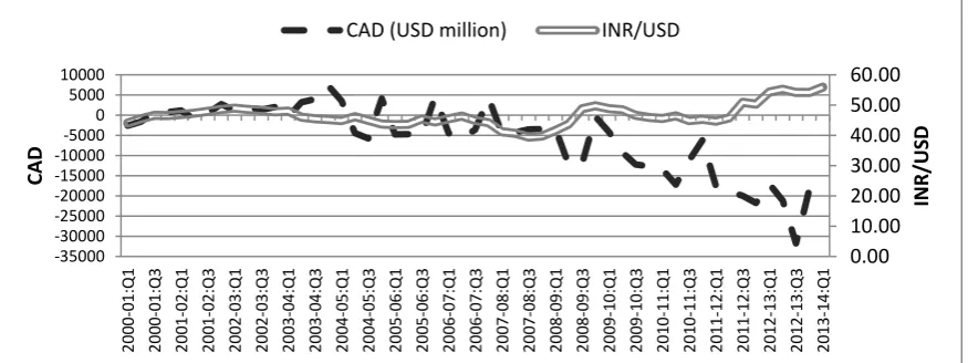
After a sharp drop as Lehman Brothers fell in October 2008, inflows resumed. But now they were barely sufficient to finance the widening CAD. Drawdown of reserves was limited so there were large fluctuations in the rupee. Even so, Figure 1 shows reserves did fall in the GFC year 2008-09. Foreign currency accumulation soon restarted but increments in reserves were small since inflows now about equaled the CAD. Table 1 shows this for Q1 and Q2 2011-12. But in Q3, as the Euro debt crisis escalated, inflows fell far short of a widening CAD. The Reserve Bank of India (RBI) sold some reserves, but the rupee slumped to 552. Inflows revived somewhat in Q4 (Table 1) and the rupee, came back towards 50. But the CAD was not necessarily responsible for the depreciation of the INR. There were periods when deterioration did not provoke an outflow and depreciation (Figure 2). The causality

could be the reverse, with sharp depreciation due to risk-off capital outflows widening the CAD by increasing the import bill.

Although the capital plus the current account must equal the change in reserves, a tautology does not imply causality. Many macro variables adjust to achieve the equality. It is

sometimes said that higher capital inflows lead to higher CADs. This is possible over the longer-term if capital inflows result in real exchange rate over-valuation, but this was

generally avoided in India. It was during periods of outflows that the CAD widened. Inflows do provide a tempting short-term financing option, but they are fickle, a fact policy was generally aware of.

Figure 2: Quarterly CAD and exchange rate movements

2

For the year as a whole the CAD was 4.2% compared to capital inflows at 3.7%. The RBI’s draw-down of reserves, amounting to 12.8 billion USD, made up the difference. In 2012-13 the CAD peaked at 4.8%, before coming down the next year.

0.00 10.00 20.00 30.00 40.00 50.00 60.00 -35000 -30000 -25000 -20000 -15000 -10000 -5000 0 5000 10000 200 0-0 1:Q1 200 0-0 1:Q3 200 1-0 2:Q1 200 1-0 2:Q3 200 2-0 3:Q1 200 2-0 3:Q3 200 3-0 4:Q1 200 3-0 4:Q3 200 4-0 5:Q1 200 4-0 5:Q3 200 5-0 6:Q1 200 5-0 6:Q3 200 6-0 7:Q1 200 6-0 7:Q3 200 7-0 8:Q1 200 7-0 8:Q3 200 8-0 9:Q1 200 8-0 9:Q 3 200 9-1 0:Q1 200 9-1 0:Q3 201 0-1 1:Q1 201 0-1 1:Q3 201 1-1 2:Q 1 201 1-1 2:Q3 201 2-1 3:Q1 201 2-1 3:Q3 201 3-1 4:Q1 INR /US D CAD

6

But could domestic policy have taken measures to prevent the unprecedented widening of the CAD?

3. CAD: Excess demand or external and sectoral shocks?

That there were twin deficits, a fiscal deficit (FD) as well as a CAD, suggests there was generalized excess demand that policy could have reduced. However, even as the CAD widened in 2011-12, India’s GDP growth rate fell to 6.5 percent, compared to 8.4 percent in the previous year. Further widening of the CAD in the next year accompanied even lower growth of 5 percent. Growth in aggregate demand categories like consumption and fixed investment also fell. As against this, the CAD was only 1.3 percent in 2007-08, a year of high

consumption and investment when output grew at above 9 per cent. So it was supply shocks, not excess demand that widened the CAD. Commodity price shocks led inflation raised imports of crude oil and gold, and reduced financial savings.

Figure 3: Current account deficit and trade deficit (X-M) adjusted for oil (O) and gold (G) (ratio to

GDP)

A steep rise in commodity prices occurred despite a global slowdown, because of QE and risks in the Middle-East. Oil price shocks raised the rupee import bill, even as incomplete pass through to domestic oil prices further lowered the already low substitution elasticity for oil products. Periodic rupee depreciation raised the rupee value of imports. Thus rising CAD levels could be linked to multiple cost shocks that began with the spiralling of global food and oil prices in 2008. Their slow release through the system, given dysfunctional

-12.0 -10.0 -8.0 -6.0 -4.0 -2.0 0.0 2.0 4.0

199

9-0

0

200

0-0

1

200

1-0

2

200

2-0

3

200

3-0

4

200

4-0

5

200

5-0

6

200

6-0

7

200

0

8

200

8-0

9

200

9-1

0

201

0-1

1 P

201

1-1

2 P

201

2-1

3 P

7

administered price regimes, kept inflation high even as growth fell. Figure 3 shows subtracting imports of oil and gold from the trade deficit makes it a trade surplus3.

The CAD must equal I-S by definition. Investment falls in slowdowns, but if savings fall even more, the CAD widens. Financial savings finance investment that requires traded goods imports, while physical savings, such as in real estate, are invested more in non-traded goods. So a fall in financial savings widens the trade and current account deficits more. Financial disintermediation due to the absence of inflation hedges raises the demand for gold. This reduces financial savings as well as directly increases imports. Savings also fall as incomes fall (especially firm profits and government revenues).

In 2011-12 the CAD rose to 4.2 per cent of GDP, from 2.7 per cent the previous year – i.e. by 1.5 percentage points. Investment fell from 36.8 to 35 percent, or by 1.8 percentage points, while savings fell more from 34 to 30.8 or by 3.2. The largest fall in a savings component was in household financial savings from 10.4 to 8 per cent, or by 2.4 percentage points. This, together with fall in corporate saving of 0.7, itself almost entirely covers the rise in CAD and fall in investment. Household physical savings actually increased by 1.2 almost covering the fall in public sector saving of 1.3; both largely affect the demand for non-traded goods (Goyal, 2013a). There was public sector dissaving due to post GFC fiscal stimulus and rising oil subsidies, but the fall in household financial savings was the largest component.

The FD widened due to the coordinated global stimulus pushed by the G-20. The fiscal stimulus was kept in place too long because of the uncertain global recovery. As the

Government, concerned about rating downgrades, made a serious effort to reduce the FD in the last quarter of 2012, growth in government consumption fell to 1.9 per cent, from 8 per cent in the preceding quarter, while that for community, social and personal services as a whole fell from 7.5 to 5.4 per cent. That the fall in the FD reduced growth in services but not the CAD provides evidence government expenditure creates demand largely for non-tradable

goods, and for a varied food basket. Excess demand may be a problem only in agriculture, where supply rigidities prevent expansion to keep up with demand for food variety (Goyal, 2013b), while a depreciating INR prevented imports from offering a low cost solution.

3

But if petroleum product exports are subtracted from exports a trade deficit of about 2 per cent appears. All of

8

Analysis of cycles also supports the sectoral and external shocks explanation for the widening of the CAD. The trade surplus (net exports, NX) is procyclical in India rather than

countercyclical as it would be if it was driven by domestic demand. Correlation of NX normalized by output and output (NX/Y with Y) is positive. NX/Y tends to fall in periods of low growth, associated with low external demand, rather than falling when rising growth and domestic demand raise imports (Goyal, 2011).

Such an inverse relationship between the CAD and growth can occur if as exports rise they raise growth and NX. On the other hand, a sudden collapse of export markets, due to a global shock, reduces growth and decreases NX. If oil shocks raise costs, and set in a contraction,

NX would again fall along with falling growth as imports rise. The period after the financial crisis saw both a collapse in export markets and a rapid resumption in oil price hikes. These external shocks drove the trade deficit.

The post GFC experience lends itself to the following causal inferences:

1. External shocks were largely responsible for the widening of the CAD. These included fall in world export demand, and rise in oil prices given inelastic import demand. The latter, together with sectoral bottlenecks, raised domestic inflation and reduced domestic financial savings. Sharp depreciations due to risk-off outflows4, further raised the import bill and the CAD.

2. Although India required a higher level of inflows to finance a widening CAD, it was the fall in inflows, not the CAD that was primarily responsible for rupee depreciation. When inflows were plentiful, CADs were financed without depreciation.

3. But there was a vicious cycle since countries with higher CADs tended to experience more outflows during risk-off periods, which led to depreciation that worsened the CAD.

4. Policy failures

Even if external and sectoral shocks, rather than excess demand, were largely responsible for the widening CAD, there was aggravation from policy mistakes. The government did not act to alleviate sectoral bottlenecks, instead squeezing aggregate demand. It also allowed too much exchange rate and interest rate volatility.

4

9

Domestic supply bottlenecks raised coal imports, just as faltering world demand reduced general export demand. The administered pricing regime reduced substitution away from expensive imports. A paucity of inflation protected savings instruments reduced financial savings and increased the demand for gold imports. Absence of action, on constraints in agricultural marketing, boosted food inflation.

Although crude oil dominates the import basket, a structural rise in imports does occur with higher growth. Ultimately, exports have to rise to finance these. Policy that relies on

depreciation to stimulate exports, without building export capacity and lowering costs is

inadequate. For example, India’s per container trade costs are more than twice the East Asia average. Bureaucratic delays and hurdles prevent it becoming part of Asian export supply chains.

The short-term imperative of financing the CAD, led to excessive policy focus on increasing these inflows, in a departure from earlier caution. But inflows carry the risk of reversals which contributed to the external shocks India faced. Inflows also build-up debt that has to be eventually repaid by running a current account surplus. They induce excessive exchange and interest rate movements that hurt aggregate demand. The larger debt flows allowed

conservative voices pushing for the interest rate defence of the exchange rate to win the argument, although such a defence continued to be inappropriate in Indian conditions. Leaving the rupee wholly to markets over 2009-11 was another major policy mistake. Later experience showed many types of action were possible.

Absence of adequate steps to reverse the exit of domestic households from capital markets, led to FPI driven volatility dominating domestic markets. Volatility could have been reduced if the domestic retail debt had first been developed, offering more instruments suiting

household needs. This would also have raised the share of household financial savings.

Market participation of domestic pension funds could also have been liberalized.

4.1 Composition and consequences of capital flows

10

restrictions on debt, especially short-term debt, inflows5. The rationale was that even though equity flows are volatile they are at least risk sharing, while debt outflows impose a greater burden in downturns. China kept restrictions on all types of capital flows while liberalizing direct investment. India chose a different combination since it had more domestic industry to protect. Short-term debt is riskier since it is difficult and expensive to roll it over at crises times, as asset values fall and the currency depreciates. Moreover, higher growth attracts equity flows, and lower interest rates encourage growth. But debt flows come into government or corporate debt funds to earn an interest differential, so outflows affect domestic interest rates in addition to the exchange rate. Policy has to raise interest rates to retain debt flows, thus hurting growth, as well as equity flows. The inflationary impact of

depreciation and rising risk premiums can stall a policy rate cutting cycle. Depreciation also reduces returns on FPI.

Figure 4 shows the fluctuations in foreign portfolio investment (FPI), that came in through foreign institution investors (FIIs) or their sub-accounts registered with the regulator, and the steadier increase in foreign direct investment (FDI). Fluctuations in non-resident Indian deposits reflect interest rate arbitrage limited by shifting policy caps on interest rates.

Figure 4: Capital inflows to India (ratio to GDP)

Restrictions were tightened when there was a surge in aggregate capital inflows, and relaxed when inflows slowed. Controls on outflows by residents were relaxed only very gradually,

5

In 2011, for example, an FII could invest up to 10% of the total issued capital of an Indian company. The cap on aggregate debt flows from all FIIs together was 1.55 billion USD. This was increased to 30 billion to facilitate financing of the CAD. A given percentage of GDP implies very different absolute levels of inflows by the end of a period of rapid GDP growth –the absorptive capacity of the economy also rises. Inflows could only come through FIIs- individuals could not invest directly.

-1.5 -1.0 -0.5 0.0 0.5 1.0 1.5 2.0 2.5 3.0 199 0-9 1 199 1-9 2 199 2-9 3 199 3-9 4 199 4-9 5 199 5-9 6 199 6-9 7 199 7-9 8 199 8-9 9 199 9-0 0 200 0-0 1 200 1-0 2 200 2-0 3 200 3-0 4 200 4-0 5 200 5-0 6 200 6-0 7 200 7-0 8 200 8-0 9 200 9-1 0 201 0-1 1 201 1-1 2 201 2-1 3

11

initially only for current account transactions. Globally, the most volatile cross border flows around the period of the GFC were inter-bank flows—India’s conservative bank open position limits and restrictions on intermediary flows protected it from excess volatility on this count. Equity inflows dominated because of caps on debt inflows. These must continue until fundamentals improve and domestic markets deepen.

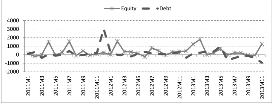
Figure 5: Monthly equity and debt inflows (USD million)

Post 2011 imperatives of financing the CAD did lead to unwarranted relaxations in debt flows. By 2013 caps on government debt for foreign investors had been raised to USD 30 billion (overall debt limit including corporate bonds at 81 billion). Expansion of external commercial borrowings (ECBs), to facilitate domestic firms borrowing abroad, meant domestic firms were carrying more and more currency risk. Figure 5 shows outflows after

Bernanke’s May 2013 statement were largely in the debt component. Outflows occurred because of an expected strengthening of US bond yields, on earlier withdrawing of QE. Indian market positions were largely long in government debt as interest rates were in a downward phase. But yields rose with the policy response to debt outflows that raised short rates by 300 basis points. There were large domestic market losses as bond values fell.

But even in September 2013, after relaxation in debt caps, the share of debt securities was still small at 36 per cent of equity securities and 6 per cent of total liabilities. So the rise in yields was driven more by unnecessary policy tightening, not the debt outflows, in the Indian context6. Policy did not utilize degrees of freedom from the careful sequencing of capital

6

Debt outflows over May 22-August 26th were 868 USD million for Indonesia, where foreign funding of domestic currency sovereign bonds had been liberalized considerably, compared to 35 USD million for India.

-2000 -1000 0 1000 2000 3000 4000

20

11M1

20

11M3

20

11M5

20

11M7

20

11M9

20

11M1

1

20

12M1

20

12M3

20

12

M5

20

12M7

20

12M9

20

12M1

1

20

13M1

20

13M3

20

13M5

20

13M7

20

13M9

20

13M1

1

12

account convertibility. Research at the IMF (2014) showing bond mutual funds, especially retail funds, are twice as sensitive as equity mutual funds to global sentiment, underlines the wisdom of the sequencing7.

Figure 6: India’s income payments abroad (-) (ratio to GDP)

Table 2: Overall international investment position of India (USD billion)

2009-Sep 2010-Sep 2011-Sep 2012-Sep 2013-Sep

(PR)

Assets 375.9 406.9 434.7 441.9 436.7

of which

Direct Investment 76.5 91.5 109.1 115.9 120.1

Reserve Assets 281.3 292.9 311.5 294.8 277.2

Liabilities 482.5 611.9 659.6 713.4 736.2

of which

Direct Investment 159.3 197.8 212.9 229.9 218.1

Portfolio Investment 106 163.8 161.5 164.6 171.6

Equity Securities 85.1 130.5 128 125.7 124.3

Debt Securities 20.9 33.3 33.5 39 47.3

Other Investment 217.1 250.4 285.2 318.9 346.5

Trade Credits 41.9 56.6 66.7 76.9 89.6

Loans 120.7 134.8 158 164.8 168.7

Currency & Deposits 46.7 50.5 52.4 67.2 75.2

Other Liabilities 7.9 8.5 8.1 10 13.1

Source: Macroeconomic and Monetary Developments, table III.2Major items of India’s balance of payments www.rbi.org.in

So Indonesia had to raise policy rates 175 basis posts post taper-on. IMF (2013) in a regression of domestic on US yields finds a significant coefficient (1.1) for Indonesia compared to insignificant (-0.3) for India.

7

In a sensible application of this logic, the RBI in 2014 disallowed FPI investments in G-Secs of less than one year maturity, in anticipation of possible future taper-related volatility.

-2.00 -1.50 -1.00 -0.50 0.00 0.50 195 0-5 1 195 2-5 3 195 4-5 5 195 6-5 7 195 8-5 9 196 0-6 1 196 2-6 3 196 4-6 5 196 6-6 7 196 8-6 9 197 0-7 1 197 2-7 3 197 4-7 5 197 6-7 7 197 8-7 9 198 0-8 1 198 2-8 3 198 4-8 5 198 6-8 7 198 8-8 9 199 0-9 1 199 2-9 3 199 4-9 5 199 6-9 7 199 8-9 9 200 0-0 1 200 2-0 3 200 4-0 5 200 6-0 7 200 8-0 9 201 0-1 1

13

Overtime capital flows affect international debt or, as it is known in India, the country’s

International Investment Position (Table 2). India’s strategic choices in capital account convertibility imply liabilities comprise mostly FDI and foreigner’s equity holdings. Assets largely reflect the rise in foreign exchange (FX) reserves, and some outward FDI. The reserves are sufficient to cover short term outflows particularly since equity outflows would reduce in value during a concerted exit. Even so, the short-term debt component has risen above 40 percent, in residual maturity terms, which is unhealthy. The rising debt and share of FIs played a role in convincing authorities that markets were too large and reserves too small for the RBI to intervene. But this was an incorrect conclusion since reserves were still large compared to volatile components such as foreign liabilities, debt and equity securities (Table

2). Indian reserves satisfied various criteria of reserve adequacy used such as comparing them to the sum of short-term external debt plus CAD, or CAD minus FDI inflows. Indeed the IMF regarded Indian reserves as too large

As a country continues to borrow more abroad than it lends, it has to service the debt. So its gross national product (GNP) is less than its GDP. Net income paid abroad has to be

deducted from GDP produced within a nation’s boundary to obtain the nation’s GNP. Figure 6 shows the adjustment as a ratio to GDP. Although the adjustment is negative, the amount is low, only about minus half a percentage point. Despite rising debt, the ratio stayed constant in recent years because a rise in GDP and fall in global interest rates reduced net interest and service payments. These can, however, rise rapidly as global interest rates rise. So borrowing must be used productively.

5. Reducing the impact of external shocks on the exchange rate

Risk premiums are volatile in thin EM markets. Capital flows that respond to global not to domestic conditions, also aggravate the tendency for exchange rates to overshoot

fundamental values, so the value of the currency cannot be left to markets alone. The academic literature also has shifted away from advocating corner regimes of a full float or

14

Unfortunately, just as strong global risk-on risk-off in the period after the GFC created perverse movements in the exchange rate, policy became increasingly hands off. Although the stated position remained the RBI would act to prevent excess volatility, markets were allowed to determine INR level and volatility subject to what remained of capital controls that were being reduced under domestic and international pressure. Intervention was

temporarily suspended in 2007 at a time of strong inflows that made sterilization difficult, but resumed to accumulate inflows from October as the market stabilization bonds were

negotiated for cost sharing with the government. The INR had to depreciate during post-Lehman equity outflows in order for them to take a write-down in asset values and share risk. The RBI did sell some reserves. Inflows resumed quickly, however, and upto end 2011, were

just adequate to finance the CAD (Figure 1). So there was hardly any intervention in this period. This led to the market misperception that the RBI was unable to intervene in FX markets, aided by statements from the RBI about the large size of India’s FX liabilities and potential capital movements relative to reserves. As a result the rupee went into a free fall in end 2011. An environment of low growth and a rising CAD added to the fragility of FX markets.

There is an argument that hands off during depreciations contributes to an undervalued real exchange rate that helps exports. But a fall in export growth and a widening CAD

accompanied depreciation from INR/USD 45 in early 2011 to 67 in September 2013, when depreciation is supposed to improve both CAD and exports (see the qualifications to this argument in Box 1). In October 2013 the INR recovered to 62, but exports began to grow as global growth revived. High volatility, such as a sharp depreciation, does not help exporters.

Depreciation corrects for inflation differentials but itself contributes to inflation, as imports and import substitutes become costly, so real depreciation is much lower. Instead a vicious cycle of higher inflation requiring more depreciation sets in. Repeated bouts of sharp

depreciation contributed to sticky Indian inflation, and hardened inflation expectations. Post

the 2011 depreciation, growth fell while inflation remained high and sticky.

15

100) stood at 95 and 87.3 in end December (RBI 2014). Prior to this, over 2010-11 and 2011-12 there was mild real appreciation—the 36-country REER rose to 103.9 and 101.4

respectively. But export growth was 21.8% in 2011-12 and collapsed to -1.8 the next year with the slowdown in Europe. The brief appreciation cannot be blamed for the export slowdown and CAD widening. It was global demand effects that dominated.

BOX 1: Re-switching: Does depreciation reduce a CAD?

The real exchange rate affects exports and imports depending on the elasticity of demand. The Marshall-Lerner condition says that depreciation will improve a CAD only if the sum of import and export elasticity of demand exceeds unity in absolute terms. There is also

evidence of immediate worsening of the CAD with improvement after a lag. This J-curve occurs if price contracts take time to be re-negotiated. Since for an EM imports are often priced in dollars and exports in domestic currency, the initial impact of depreciation only raises the import bill. The CAD deteriorates. If exporters have less market power, they may not be able to get the higher domestic currency prices required to stimulate exports, even in the long-run.

If the pass through from depreciation to domestic prices is high, inflation appreciates the real exchange rate and real depreciation is limited. The pass through tends to be higher for

commodities such as oil, which are contracted in dollar prices, and for differentiated goods imports such as high quality capital goods for which competition is limited. These dominate the Indian import basket. It is also higher in times of high inflation, for large spikes and persistent changes in the exchange rate since menu costs of price change are then exceeded (Ghosh and Rajan, 2007). Mallick and Marques (2008) also find the pass through to import prices to be high in India.

The global cycle also matters. In a period of low global demand depreciation cannot increase exports, so only adds to import costs. In the UK also the pound depreciated 20 per cent since

16

But in the UK policy interest rates were kept low and this, together with a floating exchange rate, allowed the government to borrow at much lower rates than most countries under the Euro. For example, the UK ten year bond yield was only 2.5 percent in 2013. In AEs with free floats and capital flows interest parity forces instant over depreciation, the expected future appreciation allows domestic interest rates to be below foreign rates while equating the returns to capital. EMs do not have this facility, since sustained depreciation tends to raise country risk. For EM currencies it tends to lead not to expected appreciation back towards fundamentals but to fears of further weakening. So taking a sharp INR depreciation need not even facilitate lower interest rates.

Over the longer-term, an undervalued real exchange rate does increase exports, as the

Chinese experience demonstrates. But to be sustained it requires a disciplined labour market, where real wages do not rise. Chinese wages rose after many years of high growth, but Indian wages began to rise much earlier in the Indian catch-up cycle. The rise in Indian real wages over 2007-13 years requires real appreciation, which has to occur through inflation if there is nominal depreciation. And indeed, as wages continued to rise, inflation intensified after a sharp 2011 depreciation reversed earlier real appreciation. In Indian conditions a steady competitive REER, may be feasible, but undervaluation is difficult to sustain. Such a REER may be adequate to maintain healthy export growth, with complementary supply side

measures.

….

The RBI did begin to sell reserves in November 2011 as the INR spiralled downwards. It also restricted FX markets. Retrospective taxation in budget 2012, and the Fed’s taper

announcement in May 2013, all led to outflows requiring RBI action8. Some of many feasible policy actions, including administrative measures such as controls, market restrictions,

intervention or buying and selling in FX markets, signalling, and monetary policy measures such as the classic interest rate defense were used.

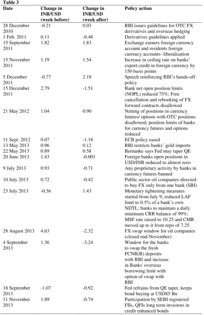
Table 3, which lists the policy measures taken over 2010-2013, attempts to assess their effectiveness by estimating the impact on the exchange rate, that is, did a measure reverse or

8

17

add to existing market movements? The Table gives the basis points change in the INR/USD rate in the week before and the week after a measure. A negative entry implies an

appreciation of the INR and a positive entry the reverse. Table 3

Date Change in

INR/USD (week before)

Change in INR/USD (week after)

Policy action

28 December 2010

-0.21 0.03 RBI issues guidelines for OTC FX

derivatives and overseas hedging

1 Feb. 2011 0.11 -0.48 Derivatives guidelines applied

15 September 2011

1.82 1.83 Exchange earners foreign currency

account and residents foreign currency accounts- liberalisation 15 November

2011

1.19 1.54 Increase in ceiling rate on banks’

export credit in foreign currency by 150 basis points

5 December 2011

-0.77 2.18 Speech reinforcing RBI’s hands-off

policy 15 December

2011

2.79 -1.51 Bank net open position limits

(NOPL) reduced 75%; Free cancellation and rebooking of FX forward contracts disallowed

21 May 2012 1.04 0.90 Netting of positions in currency

futures/ options with OTC positions disallowed; position limits of banks for currency futures and options reduced

11 Sept. 2012 0.07 -1.18 ECB policy eased

13 May 2013 0.96 0.12 RBI restricts banks’ gold imports

22 May 2013 0.89 0.58 Bernanke says Fed may taper QE

20 June 2013 1.43 -0.001 Foreign banks open positions in USD/INR reduced to almost zero 9 July 2013 0.93 -0.71 Any proprietary activity by banks in

currency futures banned

10 July 2013 0.72 -0.42 Public sector oil companies directed to buy FX only from one bank (SBI)

23 July 2013 -0.36 1.43 Monetary tightening measures

started from July 9; reduced LAF

limit to 0.5% of a bank’s own

NDTL; banks to maintain a daily minimum CRR balance of 99%; MSF rate raised to 10.25 and CMR moved up to it from repo of 7.25. 28 August 2013 4.63 -2.32 FX swap window for oil companies

(closed end-November) 4 September

2013

1.36 -3.24 Window for the banks

to swap the fresh FCNR(B) deposits with RBI and increase in Banks' overseas borrowing limit with option of swap with RBI

18 September 2013

-1.07 -0.92 Fed refrains from QE taper, keeps

bond buying at USD85 Bn 11 November

2013

1.89 -0.74 Participation by SEBI registered

18

The Table indicates the most effective measure was the FX swap window announced for oil marketing companies in end August 2013. Not only did the INR strengthen substantially, but it reversed an existing depreciation. The rupee continued to gain after that, as other measures were added to the swap window that remained open till end November. Measures that made more FX available, such as the swap window and subsidy for banks foreign borrowing or easier ECB also appreciated the INR; restrictions on markets such as reducing position limits worked only sometimes. The use of the interest rate defense in July 2013 was a total failure. Signals that the RBI was unable to intervene and the INR should be left to the markets had a large impact but were also counter-productive. Well-designed signals could, therefore, have

the desired effect. Global shocks such as Fed announcements also impacted the INR.

The lessons from this experience are the importance of designing policy in line with the current state of capital account convertibility and evolution of markets. Given India’s growth prospects and relatively greater reliance on growth driven equity flows, the interest rate defense is counter-productive at the current juncture and should be avoided, even as restraints continue on debt flows. Equity investors’ assets loose value with a sharp depreciation, but an ineffective interest rate defense does not help existing equity investors, even as reduced growth harms new entrants.

Under adverse expectation driven outflows the market demand and supply for FX will not determine an exchange rate based on fundamentals. Smoothing lumpy foreign currency demand in a thin and fragile FX market is important. Direct provision of FX to oil marketing companies was first used in the mid-nineties9. It is a useful way to provide FX reserves to a fragile market without supporting departing capital flows. It showed there are innovative ways of using reserves, which can be built up again during periods of excessive inflows. Although swaps add exchange rate risk to the RBI’s balance sheet, it need not materialize over the short life of the swap if markets are successfully calmed. They also encourage

domestic entities to hedge. It is only if these polices are not used effectively that restricting markets may become necessary10. But that should be avoided, to the extent possible, since it

9

I thank Dr. Y.V. Reddy for this point. 10

Thus in December 2011, the INR remained under pressure despite a reduction in global risk-on due to ECB announcement of support to bank lending and money market activity (see

19

has adverse side-effects. Actions appropriate to the Indian context and reform path, were the most effective. Following such a restraint also reduces regulatory discretion that in a

complex environment can lead to over- or under kill.

5.1 Domestic markets

The repeated scams and financial mishaps of the nineties demonstrated the fragility of a controlled system. Therefore financial reforms towards steady market deepening were

undertaken. But the global financial crisis demonstrated the wisdom of India’s slow and steady approach to market development, and the necessity of prudential regulation to reduce risk-taking. Action on the INR should be consistent with these lessons, while not reversing

cautious steps forward to further deepen domestic markets.

Figure 7: FX market turnover (USD billion)

Figure 7 shows various market restrictive measures reduced market turnover sharply in the currency derivatives markets in exchanges, while total turnover including the dominant over-the-counter (OTC) FX trading in banks also fell. This suggests the two types of markets are complements rather than substitutes. Exchanges are thought to be dominated by speculative position-taking since no real underlying is required unlike in the RBI regulated OTC markets. But in FX markets worldwide portfolio rebalancing types of transactions between market makers are normally much larger than those based on real exposures. These allow banks, as

INR back from 55 to 50. Adverse tax measures for MNCs in the March 2012 budget triggered outflows and the INR again reached 55, leading to further market restrictions in May 2012.

0 20 40 60 80 100 120 140 160 180 0 200 400 600 800 1000 1200 1-Jan -10 1-M ar -10 1-M ay -10 1-Ju l-10 1-S e p-10 1-N o v -10 1-Jan -11 1-M ar -11 1-M ay -11 1-Ju l-11 1-Se p -11 1-N o v -11 1-Jan -12 1-M ar -12 1-M ay -12 1-Ju l-12 1-Se p -12 1-N o v -12 1-Jan -13 1-M ar -13 1-M ay -13 1-Ju l-13 1-S e p-13 Tu rn o v e r at e xch an g e s To tal tu rn o v e r

Total turnover (left axis) Turnover at exchanges (right axis)

Dec 15 2011: NOPL ; no rebooking of forwards

May 21 2012: No netting with OTC; NOPL for futures & options 

9-23 July 2013: Interest rate

INR defence

20

well as small firms that may not get a good deal at banks, to lay-off risks in futures markets. But expectations are especially important in such markets and can lead to one-way positions.

Under freer capital flows, restricting domestic markets encourages transactions to migrate abroad. Although difficult to measure precisely, the non-deliverable forward (NDF) market may be above 50 per cent of the onshore market11 and rose in the period of market

restrictions. This is against the objective of developing and deepening domestic markets. Moreover, domestic regulators are unable to influence offshore markets. Therefore policy should use prudential regulation12 rather than forbid transactions, it order to avoid driving markets overseas.

Recent experience suggests the following ranking of policy actions on the exchange rate at the current state of capital account convertibility. First, address fundamental weaknesses such as large CADs that can trigger adverse expectations, second, use reserves and signalling to smooth market demand and supply. Since capital flows do not always match the net import gap, the RBI should be ready to close any short-term demand supply mismatch.

Third, the principle of light touch regulation or minimum collateral damage prioritizes prudential measures over tightening controls. Restrictions, if they become necessary, can be targeted to a specific market, using degrees of freedom from existing controls. Collecting continuous information on one-way positions and if there is evidence of excessive

speculation, increasing position limits, margin requirements or other regulatory measures are preferable to the fourth— a ban on a market or a transaction-type or fifth— to a domestic liquidity squeeze or interest rate defence. Position limits and credit curbs can prevent domestic parties shorting the rupee by borrowing in domestic markets—but credit curbs, if used, should be targeted only to specific commodities such as gold imports. If administrative measures reduce one-way positions, a general liquidity squeeze does not contribute much to reducing FX positions but it hits other markets (See Box 2).

11

There are indications offshore markets rise with restrictions on domestic markets. According to BIS (2010, 2013) net turnover from reporting dealers abroad rose from 5.4 USD bn to 6.1, while that from reporting local dealers rose from 11.5 to 12.5 over the three years (Table E10, pp. 74, and Table 11, pp. 58). OTC FX turnover outside the country rose from 50 (20.8 USD bn) to 59% (36.3USD bn) of the total (Table E6, pp. 67, and Table 6.2, pp. 43). Goyal, Jain and Tiwari (2013) find a bidirectional relationship between the two markets, which becomes unidirectional from NDF to onshore when the INR is under downward pressure.

12

21

Box 2: Policy actions and the structure of interest rates

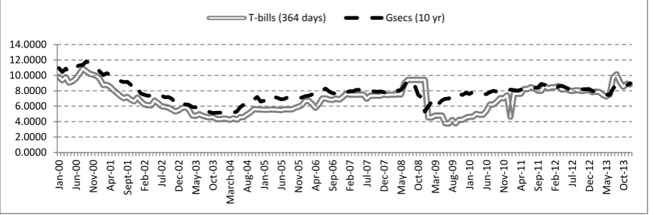
The interest rate defence works by raising the return to holding domestic currency over that to holding international currencies. If expected depreciation is large, the required rise in short-term interest rates can be very high13. To effectively impact the cost of domestic speculative borrowing the increase in short-term interest rates also has to be large.

Figure 8: Indian short and long term interest rates

Figure 8 shows the link between Indian short and long-term rates. The rise in short policy

rates in the first half of 2008, the sharp cut after the fall of Lehman Brothers, and subsequent rise all impacted long-rates.

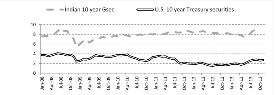
Figure 9: US and India risk spreads in basis points compared

13

The basic underlying principle is that of uncovered interest parity, which equalizes the expected returns to holding assets such as bonds in any currency (see Sarno and Taylor, 2002). Since currencies can easily depreciate by 10-40% in a crisis, short-term interest rates have to rise by as much. On 28th January 2014, even as the policy repo rate was hiked by 25 basis points there were outflows, mostly debt, due to global risk-off from

the crash of Argentina’s currency and fears of Chinese credit over-stretch. 0.0000 2.0000 4.0000 6.0000 8.0000 10.0000 12.0000 14.0000 Jan -0 0 Jun -00 N o v -00 A pr -01 S e pt -0 1 F e b-02 Jul -02 D e c-02 M ay -0 3 O ct -03 M ar ch-04 A ug -04 Jan -0 5 Jun -05 N o v-05 A pr -06 Se p -06 F e b-07 Jul -07 D e c-07 M ay -0 8 O ct -08 M ar -0 9 A ug -09 Jan -1 0 Jun -10 N o v -10 A pr -11 S e p-11 F e b-12 Jul -12 D e c-12 M ay -1 3 O ct -13

T-bills (364 days) Gsecs (10 yr)

0 100 200 300 400 500 600 700 Jan -0 8 A pr -08 Jul -08 O ct -08 Jan -0 9 A pr -09 Jul -09 O ct -09 Jan -1 0 A pr -10 Jul -10 O ct -10 Jan -1 1 Apr -11 Jul -11 O ct -11 Jan -1 2 A pr -12 Jul -12 O ct -12 Jan -1 3 A pr -13 Jul -13 O ct -13

22

The difference between interest rates on interbank loans and on risk-free, short-term

government debt (T-bills) is an indicator of rising counterparty risk, or of tightening liquidity in the interbank market. Figure 9 shows the TED spread, the difference between the 3 months US T-bill and the 3 months London Euro-Dollar Deposit Rate, and its Indian equivalent, the 3 months MIBOR (Mumbai Interbank offered rate) minus the 91 days T-bill yield. The US TED spread remains generally within the range of 10 and 50 bps (0.1 per cent and 0.5 per cent), except in times of financial crisis. A rising TED spread often precedes a downturn in the US stock market.

Figure 10: Indian 10-year G-sec yields compared to US

In India, however, these spreads are large even in non-crisis times and peak sharply during periods when markets are squeezed. That they narrowed during the years of large inflows in

the mid-2000s suggests that spreads are partly due to tight liquidity or the inability to fine tune liquidity in response to shocks in government cash balances and in foreign capital flows.

If a market is thin, there is such a large impact of a demand or a supply shock.

Curdia and Woodford (2010) argue that, in AEs, a change in spreads has implications for optimal monetary policy. A larger, persistent spread in EMs indicates a requirement for structural reform, but the changes in the spread due to liquidity shocks have to be reduced or compensated for through lower rates, together with vigilant prudential policy to prevent bubbles in thin specific markets. Liquidity tightening and use of the interest rate defense also have a larger impact in EMs to the extent large spreads raise the average level of lending rates. Thus policy should prevent a widening of already large spreads.

0 2 4 6 8 10

Jan

-0

8

A

pr

-08

Jul

-08

O

ct

-08

Jan

-0

9

A

pr

-09

Jul

-09

O

ct

-09

Jan

-1

0

A

pr

-10

Jul

-10

O

ct

-10

Jan

-1

1

A

pr

-11

Jul

-11

O

ct

-11

Jan

-1

2

A

pr

-12

Jul

-12

O

ct

-12

Jan

-1

3

A

pr

-13

Jul

-13

O

ct

-13

23

The interest rate defense raised Indian long rates (Figure 8) and intensified the industrial slump. Figure 10 shows that although Indian interest rates were much higher than US this could not prevent debt outflows—these were more sensitive to global factors. Raising

domestic interest rates to keep debt is not useful when international rates are expected to rise, and the debt is a small fraction of total foreign investments. The US takes forward interest rate guidance seriously after the 1994 mayhem in bond markets following a steep rise in policy rates—a lesson the RBI could also internalize. Raising short rates to help foreign investors can hurt domestic markets. Stock market volatility had made households averse to equity mutual funds. The rise in short-term interest rates hit debt funds. Households exited these also, further lowering financial intermediation of savings which is important for

reducing the CAD.

….

6. Exchange rate regime and inflation targeting

A full float with free capital movements suits the domestic cycle if capital flows out during a domestic downturn so the exchange rate depreciates increasing export demand and output; and vice versa during an upturn so exchange rate appreciation reduces output thus

contributing to stabilization. But capital moves due to external shocks that may be totally unrelated to domestic conditions. Movements can be unrelated to fundamentals, sentiment driven, and excessive. In thin markets, if a central bank does not buy/sell a currency that is not freely traded internationally, sharp spikes occur. These raise hedging costs. An exchange rate regime must follow a well-sequenced transition path.

In the current stage of capital account convertibility, where interest-sensitive inflows are still a small share of total inflows, the exchange rate should not directly enter the policy reaction function. The policy rate should respond to the indirect effect of the exchange rate on inflation. Alternatives such as intervention, smoothing net demand, and signalling can all be used to reverse deviations of the exchange rate from equilibrium, or prevent excessive

24

By now there is ample evidence of the impact of the interest rate on domestic aggregate demand. The steep rise in policy rates prior to GFC helped cause the crash in industrial output just as the steep cut in these rates post GFC led to an unexpectedly fast revival, and the cumulative sharp rise by October 2011 contributed to a sustained slowdown. Since the

interest rate affects output, an exchange rate regime that reduces import-led inflation would support a countercyclical interest rate responsive to the domestic cycle. There is some freedom to do this since capital mobility is not perfect and the exchange rate is flexible. The impossible trinity does not hold.

There are frequent temporary supply shocks, so the exchange rate’s potential to reverse their

effects on inflation can be acted upon when possible. In general, the exchange rate channel of monetary policy transmission has the shortest lag to inflation. Several policy instruments can be used if they are aligned so markets get a clear signal on the policy stance. Because India has an inelastic demand for imported intermediates, moderation of shocks to the exchange rate can reduce inflation. Flexible inflation forecast targeting will allow the types of exchange rate action that reduce inflation, mitigate capital movement induced volatility, and give other flexibilities to respond to supply shocks, even while better anchoring inflation expectations. For India it is a natural progression that re-orients its present multiple indicator approach towards inflation forecasting, thus converting it from an omnibus list to a consideration of the determinants of future inflation, even while retaining vital flexibilities.

Some exchange rate flexibility deepens markets and encourages hedging, but excessive volatility hurts the real sector— giving another argument for limits to exchange rate flexibility. Swings beyond a plus minus five percent invite excessive entry of uninformed traders. Markets try to make profits at the expense of the central bank (CB). Variation of a managed float in a band not less than ten per cent, prevents riskless “puts” against the CB, since then there is a substantial risk of loss if the expected movement does not materialize. Such a band worked in the European exchange rate mechanism. The central value need not be

announced and can change with inflation differentials in order to prevent real over- or under- valuation. Export competitiveness cannot be neglected when the trade deficit is large.

25

important and must be based on market intelligence covering net open positions, order flow, bid-ask spreads (when one-sided positions dominate dealers withdraw from supplying liquidity and spreads rise), turnover, and share of interbank trades.

EMs typically have less information and more uncertainty, so signalling can be effective. A variety of signals can be used. Different types of research-based estimates of equilibrium exchange rates can contribute to focusing market expectations. In addition to the inflation-differential based REER published currently, a fundamental value of the rupee based on factors such as unit labour costs and real wages could be also published.

Since the market is much larger, the RBI can now influence these expectations but cannot act totally against them. Overshooting from fundamental currency values and one-way feedback trading hurts markets also. Intervention when the market-determined level deviates from fundamentals aids market and real stability. These interventions can convey a strong signal, even without committing to a specific target exchange rate or deviating from the announced position of intervening only to prevent excess current and future volatility in FX markets and in the CAD.

7. The way forward

In the Indian context, flexibility in policy is important, given multiple shocks and constraints. Yet this flexibility can be consistent with transparent principles. Managed floating, and accumulation and use of reserves against surges in capital flows, can mitigate risks and help meet a number of policy objectives. It is not productive to copy AE floats, when the economy is not yet an AE. Acting as if the economy behaves in a text book fashion will not make it do so. Many Asian countries have developed domestic markets while actively managing their currencies.

Although the stated aim was to reduce it, INR volatility was high. More smoothing is

26

Even so, strong action on the supply-side and resolution of Indian structural issues, are also essential for stabilizing the exchange rate and the CAD, and enabling growth supporting monetary policy. For a healthy BOP in the long-run, domestic constraints that raise the cost of exports and of import substituting manufacture need to be removed, while raising domestic oil prices to reduce oil imports. Such reforms must come before any further relaxation for short-term debt flows.

AEs deliberately pumped up global asset prices to help their recovery ignoring global spillovers from these actions. The stimulus the Fed undertook helped the US make the best post-crisis recovery, showing it pays to support the real domestic cycle. AEs are answerable

largely to their domestic constituencies, but the G-20 and the IMF now have ways to pressurize them on external spillovers. It was hoped, after the May 2013 turbulence, the US taper on would be more sensitive to EM concerns. It was more carefully designed, with a focus on keeping interest rate expectations well-anchored. The reduction of USD 10 bn in December did not affect markets. But in January 2014 taper-on reduction occurred despite trouble in Argentina and Turkey and enhanced these troubles. There were calls for greater global policy coordination, to which the Indian RBI governor rightly contributed. EMs can also push for measures that reduce the financial over-leverage that leads to capital flow volatility (Goyal 2014).

But the ultimate defence against global volatility is in reducing vulnerability to crises through domestic reforms, even as in the short-term a reduced CAD and larger reserves reduce the skittishness of capital flows. The low effect on India of the January taper, or the end of US QE in October 2014, reflected the success of short-term measures taken, but the continuing necessity of longer-term measures should not be forgotten.

References

BIS (Bank for International Settlements). 2010. Triennial Central Bank Survey, Report on global foreign exchange market activity in 2010. Monetary and Economic Department, December.

---- 2013. Triennial Central Bank Survey, Report on global foreign exchange market turnover in 2013. Monetary and Economic Department, December.

27

Curdia, V. and M. Woodford. 2010. ‘Conventional and unconventional monetary policy,’ Federal Reserve Bank of St. Louis Review, July/August, 92 (4): 229-264.

Ghosh, A. and R. S. Rajan. 2007. ‘Exchange rate pass through in Asia: What does the literature tell us?’ Asian Pacific Economic Literature. 21 (2): 13-28.

Goyal, A. 2014. ‘Financial regulation and the G20: Options for India’, in The G20 Macroeconomic Agenda: India and the Emerging Economies. Parthasarthi Shome (ed). Cambridge University Press- New Delhi.

---- 2013a. ‘Behind the current account gap’, The Hindu Business Line, April 16. Available at

http://www.thehindubusinessline.com/opinion/columns/ashima-goyal/?pageNo=1

---- 2013b. ‘Balance of payments and imperatives of capital inflows’. In MEDC Economic Digest- Challenges of India's balance of payments, 42(8): 16-19, June

---- 2011. ‘Exchange rate regimes and macroeconomic performance in South Asia’, chapter 10 in Raghbendra Jha (ed.), Routledge Handbook on South Asian Economies, pp. 143-155, Oxon and NY: Routledge.

Goyal, R., R. Jain and S. Tewari. 2013. ‘Non deliverable forward and onshore Indian rupee market: A study on inter-linkages’. RBI working paper W P S (DEPR): 11 / 2013. Available

at http://rbidocs.rbi.org.in/rdocs/Publications/PDFs/11WPSN201213.pdf

IMF (International Monetary Fund). 2014. How do changes in the investor base and financial deepening affect emerging market economies? Chapter 2 in Global Financial Stability Report: Moving from Liquidity- to Growth-Driven Markets. Available at

http://www.imf.org/External/Pubs/FT/GFSR/2014/01/pdf/c2.pdf. Accessed on April 4, 2014.

---- 2013. Global impact and challenges of unconventional monetary policies. IMF Policy Paper. October.

Mallick, S. and H. Marques. 2008. ‘Pass-through of exchange rate and tariffs into import

process of India: Currency depreciation versus import liberalization’. Review of International Economics. 16 (4): 765-782.

RBI (Reserve Bank of India). 2014. Macroeconomic and Monetary Developments: Third Quarter Review 2013-14, January.