Characterisation of inorganic materials using solid state NMR spectroscopy

(1)

CHARACTERISATION OF INORGANIC MATERIALS

USING SOLID-STATE NMR SPECTROSCOPY

Scott Sneddon

A Thesis Submitted for the Degree of PhD at the

University of St Andrews

2016

Full metadata for this item is available in Research@StAndrews:FullText

at:

http://research-repository.st-andrews.ac.uk/

Please use this identifier to cite or link to this item: http://hdl.handle.net/10023/8239

This item is protected by original copyright

(2)

Characterisation of Inorganic Materials using

Solid-State NMR Spectroscopy

Scott Sneddon

This thesis is submitted in partial fulfilment for the degree of PhD

at the

University of St Andrews

(3)

(4)

Declaration

1. Candidate’s declarations:

I, Scott Sneddon, hereby certify that this thesis, which is approximately 71,000 words in length, has been written by me, and that it is the record of work carried out by me, or principally by myself in collaboration with others as acknowledged, and that it has not been submitted in any previous application for a higher degree.

I was admitted as a research student in September 2011 and as a candidate for the degree of PhD in September 2012; the higher study for which this is a record was carried out in the University of St Andrews between 2011 and 2015.

Date: Friday, September 25, 2015.

Signature of candidate ...

2. Supervisor’s declaration:

I hereby certify that the candidate has fulfilled the conditions of the Resolution and Regulations appropriate for the degree of PhD in the University of St Andrews and that the candidate is qualified to submit this thesis in application for that degree.

(5)

3. Permission for publication:

In submitting this thesis to the University of St Andrews I understand that I am giving permission for it to be made available for use in accordance with the regulations of the University Library for the time being in force, subject to any copyright vested in the work not being affected thereby. I also understand that the title and the abstract will be published, and that a copy of the work may be made and supplied to any bona fide library or research worker, that my thesis will be electronically accessible for personal or research use unless exempt by award of an embargo as requested below, and that the library has the right to migrate my thesis into new electronic forms as required to ensure continued access to the thesis. I have obtained any third-party copyright permissions that may be required in order to allow such access and migration, or have requested the appropriate embargo below.

The following is an agreed request by candidate and supervisor regarding the publication of this thesis:

No embargo on print copy or electronic copy.

Signature of candidate ...

(6)

Acknowledgments

I first wish to thank my supervisor, Sharon Ashbrook, for giving me this incredible opportunity to undertake a research project with her. Your patience with my many dramas, ‘quick questions’ and life ‘crises’ over the last four years is admirable. Your constant reassurance and guidance have helped me enormously and for that I thank you very much.

I would also like to thank both Sharon Ashbrook and Daniel Dawson for patiently reading my thesis. I have said from the beginning that I would get the following words into my thesis, and here they are: concomitant, gregarious, fortuitous, surreptitiously, recalcitrant and incredulous. Definitions are available upon request; just do not ask me to use those words in a sentence. I also wish to thank Becky Salt-Mountain and her cat, Muffin, for reading (and providing paw prints) over the initial chapters of my thesis.

To the members (and previous members) of the Ashbrook Group, I would first like to Valerie Seymour for being my ‘rock’ and hiking partner, Giulia Bignami for inspiring me to go to the gym and supervising my meals, and, in addition, John Griffin for patiently tutoring me the theory of NMR. I wish to thank also Ian Barnett and Robert Moran for their skills during their undergraduate research projects within the Group.

(7)

adventure to the end. To Charmaine Duthie and Pam Duncan, I would like to thank you for your unwavering support through some difficult times in my life.

To members of my family, Elizabeth Sneddon, my grandmother (Margaret Sneddon), Shonagh Threlfall and Jean Walker, I would like to thank you for providing me with much needed food and a bed.

Finally, to my mother (Helen Sneddon) and father (David Sneddon) (and occasionally my brother (Alan Sneddon), I wish to thank you for always providing me much needed emotional and financial support, often at very short notice, throughout my time here at St Andrews. Wherever the wind may take me, I know that you are always a phone call away.

(8)

To see a world in a grain of sand, And a heaven in a wild flower,

Hold infinity in the palm of your hand,

And eternity in an hour.

(9)

(10)

Abstract

This thesis uses solid-state nuclear magnetic resonance (NMR)

spectroscopy and density functional theory (DFT) calculations to study local structure and disorder in inorganic materials. Initial work concerns

microporous aluminophosphate frameworks, where the importance of

semi-empirical dispersion correction (SEDC) schemes in structural optimisation using DFT is evaluated. These schemes provide structures in

better agreement with experimental diffraction measurements, but very

similar NMR parameters are obtained for any structures where the atomic coordinates are optimised, owing to the similarity of the local geometry.

The 31_{P anisotropic shielding parameters (}_Ω_and_{κ) are then measured}

using amplified PASS experiments, but there appears to be no strong correlation of these with any single geometrical parameter.

In subsequent work, a range of zeolitic imidazolate frameworks (ZIFs) are investigated. Assignment of 13_{C and}15_{N NMR spectra, and}

measurement of the anisotropic NMR parameters, enabled the number

and type of linkers present to be determined. For 15

N, differences in Ω may

provide information on the framework topology. While 67_Zn

measurements are experimentally challenging and periodic DFT

calculations are currently unreliable, calculations on small model clusters

provide good agreement with experiment and indicate that 67_{Zn NMR}

spectra are sensitive to the local structure.

Finally, a series of pyrochlore-based ceramics (Y2Hf2–xSnxO7) is

investigated. A phase transformation from pyrochlore to a disordered

defect fluorite phase is predicted, but 89

Y and 119

(11)

maximum of ~12% Hf incorporated into the pyrochlore phase. The use of

17

O NMR to provide insight into the local structure and disorder in these materials is also investigated. Once the different T1 relaxation and nutation

behaviour is considered it is shown that quantitative 17_{O enrichment of}

Y2Sn2O7 is possible, and that 17O does offer a promising future tool for

(12)

Publications

S. Sneddon, D. M. Dawson, C. J. Pickard and S. E. Ashbrook, Phys. Chem. Chem. Phys., 2014, 16, 2660-2673.

S. E. Ashbrook and S. Sneddon, J. Am. Chem. Soc., 2014, 136, 15440-15456.

S. E. Ashbrook, M. R. Mitchell, S. Sneddon, R. F. Moran, M. de los Reyes,

G. R. Lumpkin and K. R. Whittle, Phys. Chem. Chem. Phys., 2015, 17,

9049-9059.

J. Cepeda, S. Pérez-Yáñez, G. Beobide, O. Castillo, A. Luque, P. A. Wright,

(13)

(14)

Chapter One

Characterisation of Inorganic

Materials by Solid-State NMR

Spectroscopy

1.1 Introduction

Since its discovery, some 70 years ago, independently by both Bloch1

and

Purcell,2_{Nuclear Magnetic Resonance (NMR) has revolutionised the way}

molecules and complexes are analysed, characterised and understood.

Today, NMR spectroscopy is one of the most widely-used analytical

techniques in chemistry as it is an excellent probe of local structure for

chemical systems ranging from the very small (e.g., organic and inorganic

drug molecules3,4

) to the very large (e.g., transmembrane proteins5

). NMR

spectroscopy has also transformed the way clinical imaging is performed

in hospitals and has become the diagnostic method of choice over X-ray

CT scanners owing to the non-invasive nature of the technique.6

The

wealth of information present in an NMR spectrum can provide insight

not only into how the molecule is constructed, by identifying characteristic

chemical shifts and splittings in spectral resonances, but also chemical

information about the molecule (e.g., identifying functional groups and

tautomerism).7-10_{Furthermore, a range of pulsed NMR experiments can be}

tailored by the NMR spectroscopist in order to answer more specific

(21)

In the liquid state, NMR spectral lineshapes are inherently narrow

owing to the rapid tumbling motion of molecules, which averages out

anisotropic (orientationally-dependent) interactions, such as the chemical shift anisotropy (CSA) and nuclear dipole-dipole coupling interactions,

yielding high-resolution NMR spectra. Therefore, detailed chemical

information can be easily obtained from one- or two-dimensional NMR spectra on a reasonable timescale. In the solid state, this molecular motion

does not usually occur (at least not on such timescales), therefore, atoms

and molecules can be thought of as being in typically fixed positions and, as a result, any anisotropic interactions are not averaged. The result of this

is the broadening of all spectral resonances in the NMR spectrum, making

it very difficult to obtain detailed chemical information.11

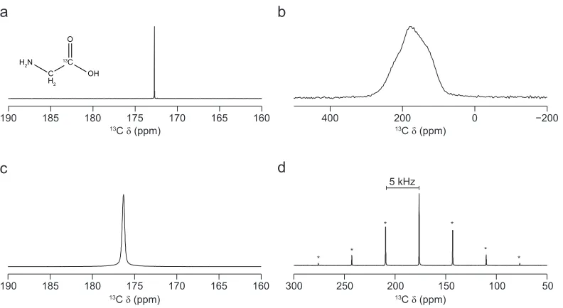
Figure 1.1 shows the differences between solution- and solid-state 13_{C NMR spectra of}13

C-enriched glycine, where the carboxylic acid carbon is C-enriched with 13

C,

giving the chemical formula NH2CH2 13

COOH. In the solution-state NMR spectrum, shown in Figure 1.1 (a), a single sharp spectral resonance,

a

170 175 180 185

190 165 160

170 175 180 185

190 165 160

c

H2N

C H2 13_C OH O b 100 150 200 250 300 50 d 5 kHz * * * * * *

13_{C (ppm)}

13_{C (ppm)} 13_{C (ppm)}

400 200 0

[image:21.595.87.483.73.290.2]

13_{C (ppm)}

Figure 1.1: 13_{C NMR spectrum of}13_{C-enriched glycine. In (a),}13_{C (11.7 T, D}

2O) solution-state NMR

spectrum. In (b-d) 13_{C (14.1 T) solid-state NMR spectra of}13_{C-enriched glycine, where the MAS rate}

(22)

corresponding to the labelled carboxylic acid functional group, is

observed at an isotropic chemical shift of 173.3 ppm, whereas for the solid sample this resonance is now broadened by the orientation-dependent

interactions, as shown in Figure 1.1 (b). As a consequence, it is very

difficult to extract any chemical information from this solid-state NMR spectrum other than the approximate peak position, of 180 ppm.

One of the major driving forces in solid-state NMR research is the need to design and implement experimental and instrumental approaches

to obtain high-resolution, solution-like NMR spectra. One of the first steps

towards obtaining high-resolution NMR spectra was the independent work of Andrew12_{and Lowe}13_{in the late 1950s. Both Andrew and Lowe}

were able to show that by physically rotating a solid sample at a fixed

angle of 54.736° with respect to a static external magnetic field, many anisotropic interactions could be averaged to zero, hence, producing

narrower spectral lineshapes in the solid-state NMR spectrum. This angle

was termed the ‘magic angle’. Since then, magic-angle spinning (MAS) experiments are now performed on a routine basis and have

revolutionised the way solid-state NMR spectra are acquired. Figure 1.1

(c) shows that by rotating a solid sample of 13

C-enriched glycine at the magic angle, the broad spectral lineshape, shown in Figure 1.1 (b), is now

considerably narrowed (from 16.7 kHz to 52 Hz). As a result of the

reduced spectral linewidth, the isotropic chemical shift of 176.3 ppm can be easily be extracted. Note the difference in isotropic chemical shift

between Figures 1.1 (a) and 1.1 (c) is due to the difference in crystal

packing of the glycine molecules in the liquid and solid state. However, the linewidth in the spectrum shown Figure 1.1 (c) is much broader than

for the same species in solution (Figure 1.1 (a)), where a peak width of 1.2

(23)

Additional resonances, termed ‘spinning sidebands’, may appear in MAS NMR spectra as a result of the incomplete averaging of the CSA.

The spinning sidebands are separated from the expected isotropic peak by

integer multiples of the MAS frequency. Figure 1.1 (d) shows the same 13

C MAS NMR spectrum as in Figure 1.1 (c), but, with a much larger spectral

width. In this spectrum, spinning sidebands are observed on either side of

the isotropic peak, each separated by 5 kHz; the MAS frequency used in this experiment. The intensity of the spinning sidebands maps out the

static powder pattern lineshape and can be extremely useful in

determining the extent of the CSA,11

which may provide additional structural information about the material, as described in more detail in

Chapter Four.

One of the most common causes of broadening of the spectral

resonances in solid-state NMR is the direct dipolar-dipole coupling

interaction. This is a through-space interaction where the magnetic field generated on one nucleus due to the nuclear magnetic moment, perturbs

that of another.14_{The interaction may be homonuclear (}_i_._e._{, between two of}

the same nuclear species, e.g., 1

H-1

H) or heteronuclear (i.e., between different nuclear species, e.g., 1_H-13_{C). Both can be removed by utilising}

MAS experiments, providing that the magnitude of the dipolar coupling

interaction is smaller than the spinning frequency.11

If the magnitude is large (compared to the spinning frequency of the rotor) broadening of

spectral resonances can be observed. For example, for strong homonuclear

and heteronuclear dipolar couplings, such as 1

H-1

H and 1

H-13

C, respectively, it is not always possible to achieve fast enough fast enough

(24)

One possible method to obtain high-resolution solid-state NMR

spectra is to ‘decouple’ the dipolar interactions by radiofrequency

irradiation to one of the coupled spins during acquisition of the signal of the other, or by applying the sequence over the entire experiment (e.g., if

two-dimensional experiments are utilised). Heteronuclear decoupling

pulse sequences, such as continuous wave (CW), have been used in solution-state NMR experiments15_{since 1955 and have since been}

developed further for solids by using more sophisticated pulse schemes,

such as two-pulse phase-modulation (TPPM) decoupling,16

or Small Phase Incremental Alternation decoupling (SPINAL-64) decoupling.17_{Figure 1.2}

(a) shows the static 13_{C NMR spectra of}13_{C-enriched glycine, where}1_H

decoupling has not been used, and Figure 1.2 (b) shows the same spectrum but with CW 1_{H decoupling applied during acquisition. As}

noted above, a broad Gaussian-like resonance is observed and was

attributed to the 13

C resonance corresponding to the carboxylic acid carbon. Figure 1.2 (b) shows that if CW 1_{H decoupling is applied during}

acquisition, the decoupling removes the Gaussian broadening from 1_H-13_C

dipolar coupling interactions but as it was not able to remove the CSA a powder pattern can now be observed. The lineshape obtained in Figure 1.2

a

400 200 0

13_{C (ppm)}

b

400 200 0

13_{C (ppm)}

Figure 1.2: Static 13_{C (14.1 T) solid-state NMR spectra of}13_{C-enriched glycine. In (a), the spectrum}

was the result of averaging 1392 transients, using a recycle interval of 3 s and acquired without 1_H

decoupling. In (b), the spectrum was the result of averaging 1024 transients, using a recycle interval of 3 s and acquired with continuous wave 1_{H decoupling, using a radiofrequency field strength}

(25)

(b) can be used in analytical fitting programs to reveal information about

the local chemical environment for that particular nuclear site. AS homonuclear dipolar coupling interactions (e.g., 1_H-1_{H) are much more}

difficult to remove by MAS experiments, and therefore, more complex,

multiple-pulse decoupling sequences are usually employed during signal acquisition to remove this interaction.18

MAS techniques can also be used to reduce the ‘quadrupolar coupling’ interactions which affects those nuclei with a nuclear spin

quantum number I > 1/2.11_{However, such quadrupolar nuclei have an}

interaction with the electric field gradient (EFG). This leads to more complex orientation-dependent interaction, described in more detail in

Chapter Two. Owing to the more complex orientation-dependence, the

quadrupolar broadening cannot be fully removed by spinning at one angle alone. Therefore, in order to obtain high-resolution NMR spectra,

more complex experiments are required, e.g., two-dimensional

multiple-quantum (MQ) MAS experiments, where the anisotropically broadened spectrum is correlated with the corresponding isotropic spectrum.19-22

Improvement in probe hardware have allowed double-rotation (DOR)23

and dynamic angle spinning (DAS)24

experiments to be performed. The former is conceptually easier to understand, where two rotors, one inside

the other, are rotated at two different angles (54.74° and 30.56°) to average

the two different anisotropic components of the quadrupolar broadening interaction. In the latter, a sample is rotated about one angle and then

rotated to a different angle for a set period of time in a two-dimensional

NMR experiment. The angles and times are chosen such that the quadrupolar broadening is refocused. The quadrupolar coupling

interaction can provide information about the coordination number of the

(26)

The ability to measure both the isotropic and anisotropic shielding

parameters could potentially reduce the challenges of assigning and interpreting solid-state NMR spectra. Initially, solid-state NMR spectra

were interpreted by comparing observed results with known reference

systems (compiled in databases consisting of many nuclei over a wide range of chemical shifts) in order to attribute each resonance to a

corresponding chemical environment.26_{Recently there has been some}

progression in assigning NMR spectra, where empirical relationships, such as bond angles and lengths, are also considered.27_{However, with the}

continued development and advancement of high-resolution solid-state

NMR experiments, the observed parameters revealed that these simple relationships could not provide the required level of accuracy for the

various systems under investigation. To date, the isotropic chemical

shift,27

dipolar28

and scalar couplings29

have been exploited in deriving the structure of a crystal. The latter two methods largely rely on the

interactions being present and are strong enough to measure

experimentally.

Measuring the isotopic shift is relatively straightforward for nuclei

with nuclear spin quantum number I = 1/2, whereas, measuring the CSA can be significantly more challenging. Measurements of the CSA can be

made using single-crystals32_{or wideline static NMR spectra of powdered}

solids.33

The former is hindered by the requirement of a sufficiently large single crystal and the need for a specialist probehead on which the single

crystal is mounted. Conversely, wideline NMR experiments suffer from

poor sensitivity and, potentially, additional broadening interactions, as seen in Figure 1.2 (a). Heteronuclear dipolar decoupling can help in

resolving the powder pattern lineshape, shown in Figure 1.2 (b). Where

(27)

then the possibility that the powder pattern lineshapes will be overlapped,

resulting in a spectrum that is far too complex for analysis.

It is often easier to measure the sideband intensities from MAS

experiments,32,33

and a number of fitting procedures have been proposed over the years in order to extract the CSA parameters in this way. One

such fitting procedure, developed by Herzfeld and Berger in the 1980s,34

utilises the magnitude of the anisotropy (span (Ω)) and the shape of the tensor (skew (κ)). This allowed plots of sideband intensities with respect to

κ and Ω/ωr, where ωr is the MAS rate, to be made and then compared with

experimental data. Hodgkinson and Emsley reported that for accurate analysis of the CSA, only five spinning sidebands, of good intensity, are

needed for the determination of Ω, but as κ approaches ±1, more spinning sidebands are needed for accurate determination.35

Measuring the CSA from MAS experiments can also be challenging due to the need to choose

a MAS rate that is neither too fast, resulting in an insufficient number of

spinning sidebands, nor too slow, which can result in broadening of the resonances in the NMR spectrum owing to the incomplete averaging of

the dipolar coupling. An additional complication is that, if there is more

than one isotropic resonance the MAS NMR spectrum, there is then the potential for the spinning sidebands to overlap, complicating or

preventing analysis. Furthermore, if the nuclear site is in a highly

symmetrical environment, the CSA will be very small and the need to spin very slowly becomes technically challenging due to the instability of the

rotor whilst spinning at such low MAS rates.

Recently, there has been much interest in measuring the CSA

using two-dimensional MAS NMR experiments.33_{There are a number of}

(28)

the spinning sideband manifolds from the different isotropic resonances.

The first two methods were developed by Dixon in 1982. The first

experiment was called ‘total suppression of spinning sidebands’ (TOSS),36

and can remove the spinning sideband manifold, resulting in

high-resolution, liquid state-like NMR spectra with only the isotropic

resonances present. The second experiment is called ‘phase-adjusted spinning sidebands’ (PASS),36,37_{where the spinning sideband manifold can}

be separated from the isotropic resonances. Both TOSS and PASS pulse

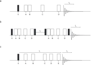
sequences are similar, shown in Figure 1.3 (a), and consist of four π pulses. However, it is the specific timings of the pulses with respect to the rotor

period that make TOSS and PASS. One of the drawbacks of PASS is that,

in order to achieve the complete separation of the sideband manifold, all peaks must have identical spin-lattice relaxation constants otherwise

distortion of the sideband intensities can be observed. Furthermore, each

PASS NMR spectrum will have to be reconstructed into a

two-a

b

c

0 A B C D

t₂

t₂ t1

0 A B C D A B C D

0 A B C E

t₁ t₂

[image:28.595.114.473.74.333.2]

D

Figure 1.3: Schematic pulse sequences of (a) the phase adjusted spinning sideband (PASS) and total suppression of spinning sidebands (TOSS) experiment,36,37_{(b) the modified PASS experiment}

developed by Lacroxi,38_{and (c) two-dimensional PASS experiment developed by Antzutkin.}39_The

(29)

dimensional NMR spectrum so that the spinning sideband manifold can

be extracted.

In 1992, de Lacroix and co-workers made a modification to the

PASS pulse sequence to include two consecutive TOSS pulse blocks, separated by an incremented t1 section, which is either 1/16 or 1/32 of the

rotor frequency, as shown in Figure 1.3 (b).38_{The first part of the pulse}

sequence evolves the magnetisation, which is then stored along the z axis during t1. The magnetisation is then returned to the transverse plane

where it is further evolved before the signal is detected during t2. The

storage of magnetisation along the z axis can result in a loss of signal by

2 . Furthermore, owing to the sequence containing many pulses,

imperfections can cause a further loss of signal and perturbations to the

spinning sideband manifold.

In 1995, Antzutkin et al. developed a pulse sequence that enabled

the spinning sideband manifolds to be separated without experiencing the problems in Dixon’s original PASS experiment and the signal loss in de

Lacroix’s pulse sequence.39_{Antzutkin’s 2D-PASS pulse sequence, shown}

in Figure 1.3 (c), is the same as Dixon’s PASS experiment, but with an additional π pulse. Another modification the authors made to the original PASS pulse sequence was to fix the duration of the PASS block. Although

the developed pulse sequence is ideal for separation of sideband manifolds, it does have one shortcoming. If the magnitude of the CSA is

very small owing to the symmetrical nature of the nuclear site, to ensure

that there are enough spinning sidebands in each manifold, then very slow MAS rates may be needed. The complications involved in using very

slow MAS rates to ensure that there are sufficient spinning sidebands has

(30)

experiments. In these experiments, the standard MAS spectrum in the

direct dimension is correlated with the corresponding slow MAS

spectrum, which has been scaled in the indirect dimension.33_Crockford_et

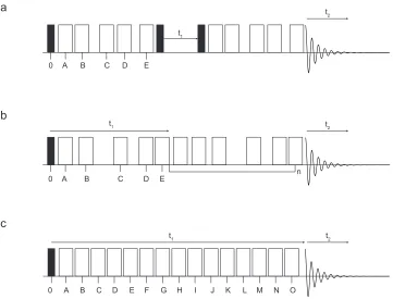
al. developed the first two-dimensional CSA-amplified PASS experiment

in 2001.40

The pulse sequence, shown in Figure 1.4 (a), is based on that of

de Lacroix et al., shown in Figure 1.3 (c), whereafter transverse

magnetisation is created, the magnetisation is manipulated by the five π

pulses, which are applied at specific timings over a number of rotor

periods (typically between one and five) before a storage period is

a

c

t₁ t₂

A B C D E F G H I

0 J K L M N O

t1

t2

A B C D E 0

t₁ t2

A B C D E n

0 b

Figure 1.4: Three approaches to the two-dimensional CSA-amplified PASS methodology. In all three examples, transverse magnetisation is created through the application of a 90° pulse (filled rectangles) and the positioning of the π pulses (open rectangles), A, B, C…etc. defines the scaling factor in which the MAS rate is scaled in the second dimension. In (a), the pulse sequence developed by Crockford et al.,40_{where the first of the five}_π_{pulses are implemented before storing}

the evolved magnetisation along the z axis during t1. The magnetisation is then allowed to evolve

through another set of five π pulses before the resulting signal is recorded as a function of t2. In (b),

the pulse sequence developed by Orr et al.,41,42_{used throughout this work, where the five}_π_pulses

allow the magnetisation to evolve over a fixed t1 time period before the resulting signal is recorded

as a function of t2. Concatenation of the first block of five π pulses, separated by a sixth π pulse,

allows for higher scaling factors to be achieved. In (c), the pulse sequence developed by Shao et al.,43

[image:30.595.113.474.71.346.2]

(31)

implemented during t1. This storage period is incremented at 1/16 or 1/32

of the rotor period. After the end of the t1 period, the same set of five π

pulses is applied to manipulate the magnetisation further before the

resulting signal is acquired in t2. One of the main disadvantages of this

pulse sequence is the 2 signal loss during the t1 storage period, as in the

pulse sequence of de Lacroix.38

In 2005, Orr et al.41

developed a different two-dimensional CSA-amplified PASS experiment that utilises the same pulse sequence of

Antzutkin et al. but with the amplification techniques developed by

Crockford.41

The pulse sequence of Orr et al. is shown in Figure 1.4 (b). Again, transverse magnetisation is created and allowed to evolve over a

fixed time period, typically four rotor periods, through the applications of

the five π pulses before the resulting signal is recorded. Concatenation of blocks of five π pulses allows higher scaling factors to be achieved, providing a sixth π pulse is applied before the next block of pulses in order to refocus the desired modulation. One of the main advantages of using this pulse sequence is that there is no signal loss during the storage period.

However, if higher scaling factors are to be achieved, concatenation of the

five π pulse block could lead to a very long pulse sequence. Orr et al. discovered that, since there is no storage period and the use of quadrature

detection is not required for the indirect dimension, twice the signal

intensity could be gained compared with methods utilising these techniques.41_{The authors later noted that total scaling factors of up to 27}

could be implemented, resulting in a loss of signal intensity of ~1/2,

which is not a disadvantage with respect to other CSA-amplified methods.42_{Finally, in 2006, Shao} _et _al_{. improved the original pulse}

sequence of Crockford et al., which is shown in Figure 1.4 (c). This pulse

(32)

the need for very long pulse sequences, and made possible with the pulse

sequence developed previously by Orr et al.43

In the solid state, atoms are typically found in fixed positions. For

a crystalline material the structure can be described by a periodic arrangement of atoms or ions in three-dimensional space. This can be

constructed from a unit cell, which can be translated according to a lattice

in three-dimensions to produce an infinite array. First proposed by William Lawrence Bragg and William Henry Bragg in 1913,44_{the study of}

solids has, for the last century, primarily been based on Bragg diffraction

experiments. These rely on the long-range order and periodicity that is typically characteristic of crystalline solids. Whilst Bragg diffraction is an

extremely powerful tool for determining the structures of crystalline

materials, many interesting properties of solids arise from a non-periodic variation in the periodic features (e.g., atomic coordinates or

substitutions/vacancies), which diffraction-based experiments often find

difficult to analyse. When a new solid is made, it is usually subjected to single-crystal X-ray diffraction, which still seen as the ‘gold standard’ for

structure determination by crystallographers. However, if suitably large

single crystals cannot be grown, then laboratory or synchrotron X-ray diffraction experiments are undoubtedly the next preferred method. These

experiments can reveal information such as the lattice type and symmetry,

and NMR is a highly complementary technique alongside such experiments. The crystal structures derived from all diffraction-based

experiments are averaged over time and distance and, generally, unable to

identify positional or compositional disorder that could be present in solid materials. Conversely, solid-state NMR is extremely sensitive to the local

structure and can provide detailed element-specific information about any

disorder or motion.11

(33)

There has been a long tradition in the solid-state chemistry

community for using computation, such as density functional theory (DFT), to help assign, interpret and understand NMR spectra of molecular

systems.45,46_{Typically, a crystal structure of the solid compound of interest}

would be obtained from either diffraction-based techniques or from a crystal structure library (e.g., from the Inorganic Crystal Structure

Database – ICSD).47_{For an extended periodic solid, a molecular cluster of}

this crystal structure would be made where any bonds that are broken or are left ‘dangling’ are terminated, typically by hydrogen atoms, in order

for the cluster to remain neutral. These terminations could potentially give

rise to structural perturbations, which in turn could result in inaccuracies in the calculated NMR parameters. The accuracy of the calculated NMR

parameters upon the cluster largely depends on its size with larger

clusters being more accurate. However, these take much longer to calculate and result in very high computational costs and so a compromise

between accuracy and computational cost needs to be made.

The 50th_{anniversary of the Hohenberg-Kohn theorem (regarded as}

the first inception of modern DFT) was marked in a series of review

articles between 2012 and 2014.48-50

DFT has become the most popular electronic structure calculation in computational chemistry. Figure 1.5

shows the number of journal papers published between January 1990 until

August 2014, where the keywords ‘density functional theory’ or ‘DFT’ appear as the topic of the paper.51_{DFT codes that utilise periodic}

boundary conditions have enabled the computation of accurate and

efficient calculations of NMR parameters by exploiting the inherent periodic nature of many crystalline solids and, therefore, avoiding the

need to approximate the solid compound of interest as a cluster. In

(34)

wave (or GIPAW)52

approach, such as CASTEP,54

have seen widespread

application for a large range of crystalline systems.45,55,56

Calculations have helped not only to understand high-resolution

spectra of nuclei with spin quantum number I = 1/2, but also for

quadrupolar (I > 1/2) nuclei. Calculation of NMR parameters have been

used to help guide experimental data acquisition, particularly for very

challenging nuclei, such as those with low natural abundance, low

sensitivity, or very large anisotropic interactions.56

Furthermore,

calculation of NMR parameters can be used to test structural models from

materials that are less well characterised using diffraction-based

techniques. The calculated results can then be compared with

experimental observations to verify the structural model. As an example,

both first-principle DFT calculations and solid-state NMR spectroscopy

were employed to determine the detailed structure of the as-prepared

form of STA-2, a microporous aluminophosphate (AlPO) material, in

which the template is charge balanced by disordered hydroxyl groups

coordinated to framework aluminium species.57

X-ray diffraction was

utilised initially to determine the crystal structure of as-made STA-2 but

the position of the charge-balancing hydroxyls had not been fully located.

(35)

By analysing 27_{Al MAS NMR spectra, it was then found that the hydroxyls}

were bridging (e.g., Al-OH-Al) and not terminal (e.g., Al-OH) in the AlPO framework. In addition, a series of structural models where the positions

of the charge-balancing hydroxyl was varied were generated in order to

probe the calculated NMR parameters and compare them with experiment.57

One challenge in the use of DFT calculations to compute NMR parameters is the requirement for a well-characterised initial structural

model. If the structure has any inaccuracies, it may then be necessary to

optimise the geometry prior to the calculation of the NMR parameters. In addition, if modifications are made to the initial structural model (e.g., the

replacement of one atom for another) then the lattice parameters and

atomic positions (determined from pervious experiments) will need to be optimised, as they will no longer be valid. DFT calculations have been

shown to play a very clear and important role in assigning, interpreting

and understanding solid-state NMR spectra and with the continual advancement in computational hardware, even more complex systems can

be investigated. Furthermore, increasing developments in computational

codes are continually providing the solid-state NMR community with more accurate calculations and new possibilities to calculate a range of

(36)

1.2 Thesis overview

This thesis describes the application of NMR and DFT to the

characterisation and understanding of a variety of inorganic materials.

Chapter Two details the theoretical background to NMR spectroscopy,

with a particular focus on solids, and describes the experiments used in

this work. Chapter Three introduces the theoretical background of

computation, focusing on using first-principles DFT codes, such as

CASTEP and Gaussian,53_{to help interpret, assign and understand}

solid-state NMR spectra.

The first section of Chapter Four describes the evaluation of the

use of two semi-empirical dispersion correction schemes on the

optimisation of the geometry of as-prepared and calcined AlPOs using the

CASTEP DFT code. Several optimisation strategies are employed,

including the optimisation of some or all atomic coordinates and

optimisation of the unit cell with and without the inclusion of the

semi-empirical dispersion correction schemes. The different optimised

structures are then compared with the initial structural model (and with

each other) by investigating the changes in the unit cell lengths, angles

and total cell volume. The calculated NMR parameters are then compared

with experimental measurements to determine the most suitable protocol

for the structural/geometry optimisation of as-prepared and calcined

AlPOs.

The second part of Chapter Four investigates the feasibility of

measuring the 31_{P CSAs of as-prepared and calcined AlPOs. Owing to the}

relatively high symmetry of the P sites in AlPOs, the use of CSA-amplified

(37)

measurement of CSAs. The results from the calculated NMR parameters

utilised in the first half of Chapter Four are then used to investigate the ability of CASTEP to calculate the CSA of a series of AlPOs accurately.

Attempts are then made to correlate the CSA with local geometrical

features, such as bond distances and angles.

Chapter Five details the characterisation of a range of as-prepared

and treated single- and dual-linker zeolitic imidazolate frameworks (ZIFs) by 1_H,13_{C and}15_{N NMR spectroscopy. DFT NMR calculations (using the}

Gaussian code) are performed on a series of isolated linker molecules in

order to assist with the assignment of the 13

C and 15

N NMR spectra. The results from measuring the 13_{C and, for the first time,}15_{N CSA parameters}

using the CSA-amplified PASS experiment are presented and correlations

between measured CSA parameters and structural features, such as topology, are considered. Chapter Five also presents some preliminary

67_{Zn solid-state NMR experiments on a small number of organic and}

inorganic Zn-containing compounds and two as-prepared ZIFs. In addition, DFT calculations (using CASTEP) are performed on a series of

Zn-containing compounds. Correlations between calculated and

experimental 67

Zn NMR parameters offer an insight to the local geometry (e.g., Zn-N bond distances and N-Zn-N bond angles) of the Zn metal

centre. As a result, cluster calculations on the first coordination sphere of

Zn using the atomic coordinates of a series of ZIFs are then performed and offer some explanation as to why it is challenging to acquire the 67_{Zn NMR}

spectra of ZIFs.

The first part of Chapter Six investigates the phase composition,

distribution and disorder of the pyrochlore ceramic Y2(Hf,Sn)2O7 using the

isotropic and anisotropic 89

Y and 119

(38)

of DFT calculations (using CASTEP) on a series of model pyrochlore

structures containing various levels of substitution of Hf and Sn enables the NMR spectra to be understood and fully assigned. The second part of

Chapter Six focuses on the cation disorder in a similar pyrochlore ceramic

material, Y2(Zr,Sn)2O7, by enriching each composition through 17O2 gas

exchange methods. The investigation of the uniformity of the 17_O

enrichment of Y2Sn2O7 and the necessary steps (both in terms of ideal

acquisition parameters and enrichment conditions) to consider in order to ensure that quantitative 17_{O NMR spectra are acquired, is presented first.}

This is then followed by 17_{O MAS NMR experiments on the whole series,}

and again using first-principles DFT calculations (using CASTEP) to interpret the NMR spectra.

Finally, Chapter Seven summaries the main conclusions of the work contained in this thesis and offers suggestions as to the future

direction of investigations into the three types of materials studied.

1.3 References

1. F. Bloch, W. W. Hansen and M. Packard, Phys. Rev., 1946, 70, 474-485.

2. E. M. Purcell, H. C. Torrey and R. V. Pound, Phys. Rev., 1946, 69, 37-38.

3.M. Pellecchia, D. S. Sem and K. Wüthrich, Nat. Rev. Drug Discov., 2002,

1, 211-219.

4. J. L. Stark and R. Powers, in NMR of Proteins and Small Biomolecules,

(39)

5. S. Wang and V. Ladizhansky, Prog. Nucl. Magn. Reson. Spectrosc., 2014,

82, 1-26.

6.E. D. Becker, Anal. Chem., 1993, 65, 295A-302A.

7. D. T. Alien, L. Petrakis, D. W. Grandy and B. C. Gates, Fuel, 1984, 63,

803-809

8. D. S. Wofford, D. M. Forkey and J. G. Russell, J. Org. Chem., 1982, 47,

5132-5137.

9. B. Wehrle, H.-H. Limbach, M. Köcher, O. Ermer and E. Vogel, Angew.

Chem. Int. Ed., 1987, 26, 934-936.

10. V. F. Traven, V. V. Negrebetsky, L. I. Vorobjeva and E. A. Carberry,

Can. J. Chem., 1997, 75, 377-383.

11. D. C. Apperley, R. K. Harris and P. Hodgkinson, in Solid-State NMR:

Basic Principles & Practice, Momentum Press, New York, 2012.

12. E. R. Andrew, A. Bradbury and R. G. Eades, Nature, 1958, 182, 1659-1659.

13. I. J. Lowe, Phys. Rev. Lett., 1959, 2, 285-287.

14. P. J. Hore, in Nuclear Magnetic Resonance, Oxford University Press, 1995.

15. A. L. Bloom and J. N. Shoolery, Phys. Rev., 1955, 97, 1261-1265.

16. A. E. Bennett, C. M. Rienstra, M. Auger, K. V. Lakshmi and R. G. Griffin, J. Chem. Phys., 1995, 103, 6951-6958.

17. B. M. Fung, A. K. Khitrin and K. Ermolaev, J. Magn. Reson., 2000, 142,

97-101.

(40)

19. L. Frydman and J. S. Harwood, J. Am. Chem. Soc., 1995, 117, 5367-5368.

20. J.-P. Amoureux, C. Fernandez and S. Steuernagel, J. Magn. Reson., 1996,

123, 116-118.

21. D. Massiot, B. Touzo, D. Trumeau, J. P. Coutures, J. Virlet, P. Florian

and P. J. Grandinetti, Solid State Nucl. Magn. Reson., 1996, 6, 73-83.

22. S. P. Brown, S. J. Heyes and S. Wimperis, J. Magn. Reson., 1996, 119,

280-284.

23. A. Samoson, E. Lippmaa and A. Pines, Mol. Phys., 1988, 65, 1013-1018.

24. K. T. Mueller, B. Q. Sun, G. C. Chingas, J. W. Zwanziger, T. Terao and

A. Pines, J. Magn. Reson., 1990, 86, 470-487.

25. S. E. Ashbrook and S. Sneddon, J. Am. Chem. Soc., 2014, 136, 15440-15456.

26. K. J. D. MacKenzie and M. E. Smith, in Multinuclear Solid-State NMR of

Inorganic Materials, Pergamon Press, Oxford, 2002.!

27. A. M. Orendt and J. C. Facelli, in NMR Crystallography, Ed. R. K. Harris,

R. E. Wasylishen and M. J. Duer, Wiley, Chichester, 2009, DOI:

10.1002/9780470034590.emrstm1044.!

28. M. R. Chierotti and R. Gobetto, CrystEngComm, 2013, 15, 8599-8612.

29. D. Sakellariou and L. Emsley, in Encyclopedia of Nuclear Magnetic

Resonance, Ed. R. K. Harris and R. E. Wasylishen, Wiley, Chichester, 2007

DOI: 10.1002/9780470034590.emrstm0566

30. M. Gee, R. E. Wasylishen, K. Eichele and J. F. Britten, J. Phys. Chem. A,

(41)

31. M. Bechmann and A. Bebald, in NMR Crystallography, Ed. R. K. Harris,

R. E. Wasylishen and M. J. Duer, Wiley, Chichester, 2009, DOI: 10.1002/9780470034590.emrstm1044.

32. J. J. Titman, in NMR Crystallography, Ed. R. K. Harris, R. E. Wasylishen

and M. J. Duer, Wiley, Chichester, 2009, DOI:

10.1002/9780470034590.emrstm1044.!

33. L. Shao and J. J. Titman, Prog. Nucl. Magn. Reson. Spectrosc., 2007, 51,

103-137.

34. J. Herzfeld and A. E. Berger, J. Chem. Phys., 1980, 73, 6021-6030.

35. P. Hodgkinson and L. Emsley, J. Chem. Phys., 1997, 107, 4808-4816.

36. W. T. Dixon, J. Chem. Phys., 1982, 77, 1800-1809.

37. W. T. Dixon, J. Magn. Reson., 1981, 44, 220-223.

38. S. F. D. Lacroix, J. J. Titman, A. Hagemeyer and H. W. Spiess, J. Magn.

Reson., 1992, 97, 435-443.

39. O. N. Antzutkin, S. C. Shekar and M. H. Levitt, J. Magn. Reson., 1995,

115, 7-19.

40. C. Crockford, H. Geen and J. J. Titman, Chem. Phys. Lett., 2001, 344, 367-373.

41. R. M. Orr, M. J. Duer and S. E. Ashbrook, J. Magn. Reson., 2005, 174,

301-309.

42. R. M. Orr and M. J. Duer, Solid State Nucl. Magn. Reson., 2006, 30, 1-8.

43. L. Shao, C. Crockford and J. J. Titman, J. Magn. Reson., 2006, 178,

155-161.

(42)

45. C. Bonhomme, C. Gervais, F. Babonneau, C. Coelho, F. Pourpoint, T.

Azaïs, S. E. Ashbrook, J. M. Griffin, J. R. Yates, F. Mauri and C. J. Pickard,

Chem. Rev., 2012, 112, 5733-5779.

46. P. J. Hasnip, K. Refson, M. I. J. Probert, J. R. Yates, S. J. Clark and C. J.

Pickard, Phil. Trans. R. Soc. A, 2014, 372, 20130270.

47. The National Chemical Database Service – ICSD, The Royal of Society

of Chemistry, http://icsd.cds.rsc.org/, accessed August 2015.

48. W. Kohn and C. D. Sherrill, J. Chem. Phys., 2014, 140, 18A201.

49. K. Burke, J. Chem. Phys., 2012, 136, 150901.

50. A. D. Becke, J. Chem. Phys., 2014, 140, 18A301.

51. Web of Science (WOK), Thomas Reuters, http://wok.mimas.ac.uk, accessed May 2015.

52. C. J. Pickard and F. Mauri, Phys. Rev. B, 2001, 63, 245101.

53. S. J. Clark, M. D. Segall, C. J. Pickard, P. J. Hasnip, M. I. Probert, K. Refson and M. C. Payne, Z. Kristallogr., 2005, 220, 567–570.

54. T. Charpentier, Solid State Nucl. Magn. Reson., 2011, 40, 1-20.

55. C. J. Pickard, in Encyclopedia of Nuclear Magnetic Resonance, Ed. R. K. Harris and R. E. Wasylishen, Wiley, Chichester, 2009, DOI:

10.1002/9780470034590.emrstm1044.!

56. L. A. O’Dell and C. I. Ratcliffe, J. Phys. Chem. A, 2011, 115, 747-752.

57. V. R. Seymour, E. C. V. Eschenroeder, M. Castro, P. A. Wright and S. E.

(43)

(44)

Chapter Two

Solid-State Nuclear Magnetic

Resonance

2.1 Introduction

In this chapter the basic principles of NMR are described in Section 2.2

with Section 2.3 describing the density operator formalism. Section 2.4

describes the internal interactions present in solid-state NMR. The

description of the many ways in which high-resolution solid-state NMR

spectra are acquired are given in Section 2.5. Finally, Section 2.6 details the

general solid-state NMR methodology used to acquire the NMR spectra

contained within this work. In addition to the specific references made

throughout this chapter, References 1-7 were used as general NMR texts.

2.2 Basic principles

2.2.1 Nuclear magnetism

All magnetic nuclei possess an intrinsic angular momentum called spin,

denoted by I, and with the bold typeface representing a vector that has

both direction and magnitude.1_{The magnitude of the angular momentum}

for a given nucleus is

| I | = ħ [ I (I + 1)]1/2

(45)

where I is the spin quantum number, which can be zero, any integer or

half-integer value, and ħ is the reduced Plank constant. For NMR

spectroscopy, the spin of the nucleus must be greater than zero. When I =

0 the nucleus possesses no magnetic moment and, hence, exhibits no

angular momentum. Projection of I onto a specified axis, arbitrarily the z

axis, is given by Iz = mI ħ, where Iz is the z component of I, mI is the

magnetic quantum number and has (2 I + 1) values between +I and −I in

integer steps. A nucleus with a non-zero spin quantum number possesses a magnetic moment, µ, which is directly proportional to I and is given by

µ = γ I_, (2.2)

where γ is the gyromagnetic ratio of the nucleus. The magnetic moment

can be projected on the z axis giving µz. In the absence of a magnetic field,

the (2 I + 1) orientations are degenerate. When place in an external

magnetic field of magnitude, B0, with direction B0, this degeneracy is

removed and each of the (2 I + 1) levels has a different energy called the

Zeeman interaction. The B0 field is defined to lie along the z axis in the

laboratory frame with the energy of each of the states becoming, E

mI

mI 0

a b

E

m_I

mI

m_I mI

mI

m_I

0

0 0 0 0 ST

ST

ST CT

Zeeman interaction

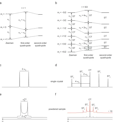
Figure 2.1: The lifting of the degeneracy of (a) I = 1/2 and (b) I = 5/2 nuclear energy levels by the Zeeman interaction with the application of an external magnetic field. The frequency difference between the energy levels is defined as the Larmor frequency, ν0, and is quoted in Hertz (Hz). In

(46)

E_m

I = µz B0 , (2.3)

E_m

I = − γ mI ħ B0 . (2.4)

The lifting of the degeneracy of the energy levels for a spin I = 1/2 and a

spin I = 5/2 by the Zeeman interaction is shown in Figures 2.1 (a) and (b),

respectively, where the energy levels are separated by (ΔE = γ ħ B0). The

selection rule for observable transitions in NMR spectroscopy is ΔmI = ± 1,

which allows transitions to occur between adjacent energy levels. The

resonance condition to move between adjacent energy levels is given by

ω0 = ΔE / ħ = − γ B0 , (2.5)

where ω0 is the Larmor frequency in rad s−1 or in Hz

ν0 =

− γ B0

2 π . (2.6)

2.2.2 The vector model

First proposed by Bloch in 1946,8_{the vector model provides a simple}

geometric interpretation to understand the basics of NMR experiments.

Despite the limitations in this approach, it is undoubtedly a useful starting

place to describe how magnetisation is manipulated in a simple NMR

experiment and enables a macroscopic ensemble of quantum mechanical

spins to be treated classically. One of the limitations of this vector model is

(47)

NMR experiments that are used within this work, and which will be

described later on in this chapter. In addition, the vector model is also not

able to adequately describe the processes that take place for quadrupolar nuclei, i.e, I > 1/2.

When a sample of interest is placed inside a magnetic field, the nuclear spins will start to populate the energy levels according to the

Boltzmann distribution.1_{This is given by}

n_upper nlower

= e−ΔEkT_, _(2.7)

where nupper and nlower describe the number of populations in the lower and

upper energy levels, k is the Boltzmann constant and T is the temperature.

Once the nuclear spins reach thermal equilibrium, there is a tendency for them to align with the field direction, leading to a net bulk magnetisation,

M0, which is aligned along the field direction and precesses about B0 at the

Larmor frequency. This phenomenon is illustrated in Figure 2.2 (a), where in the absence of a magnetic field, the nuclear spins have no preferred

orientation. However, upon the application of a strong magnetic field, the

nuclear spins will tend to align with the field direction, as shown in Figure 2.2 (b).

B₀

a b

M0

Figure 2.2: (a) In the absence of a magnetic field, all nuclei have no preferred orientation. (b) When a strong magnetic field is applied, B0, all nuclear spins will tend to align long the field direction.

(48)

In order to perturb the system and manipulate M0, a pulse of

linearly monochromatic radiofrequency (rf) is applied at a frequency (ωrf),

which is at, or close, to the Larmor frequency. This rf pulse will interact with the nuclear spins in the sample and change the orientation of M0, but

is much too difficult to visualise this interaction in the laboratory frame, as

shown in Figure 2.3. In the laboratory frame of reference, the rf pulse can be considered as two counter-rotating magnetic fields; one component

that rotates at +ωrf and the other component that rotates at −ωrf. It is often

convenient to consider the effects of an rf pulse (B1) (which is static in the

rotating frame) on M0 in which the z axis is coincident with the laboratory

z axis and the x and y axes rotate in the transverse plane (xy plane) at +ωrf.

In order to simplify the counter-rotating magnetic fields, the first component of the rf pulse (+ωrf) is static in the rotating frame, where the

frame itself is rotating at +ωrf. If visualised in this way the other

component will now be rotating twice as fast (at −2 ωrf), therefore, it

cannot interact with M0, and will now experience a magnetic field

strength, which is much smaller than B0. This smaller field is called the

effective field (Beff) and shown in Figures 2.3 (b) and (c).

a

x

y z

B₀

M0

b

B1

c

p

B_eff B_eff

Laboratory frame Rotating frame

Figure 2.3: (a) A schematic representation of the vector model, where the bulk magnetisation (M0)

along the z axis of the laboratory frame of reference. In (b) and (c), the rotating frame of reference is used to describe the effect of applying a radiofrequency pulse (of field strength B1) along the x axis.

This causes M0 to nutate through angle β. In (c), after a period of time (τp) the radiofrequency pulse

(49)

In a simple NMR experiment the rf pulse, of strength B1, is applied

orthogonal to B0, e.g., along the x axis in the rotating frame. This causes the

bulk magnetisation vector to precess in the yz plane until such a point that the rf pulse is turned off. The ‘flip angle’ (β) through which M0 nutates

under the application of the rf pulse is defined as

β = ω₁ τ_p , (2.8)

where ω₁ = − γ B₁ and τp is the duration of the pulse. The phase of the rf

pulse (ϕ) defines the direction of the B1 field in the rotating frame and the

pulses are often described in the βϕ notation, e.g., 90°x. The nutation of M0

through angle β is shown in Figure 2.3 (b). After the rf pulse has ended the

magnetisation will then start to precess in the xy plane, as shown in Figure 2.3 (c). This will be at a frequency of

Ω = ω0 − ωrf , (2.9)

where Ω is termed the offset.

The precession in the xy plane is recorded by the spectrometer to

give the ‘free induction decay’ (FID) and cannot last forever owing to relaxation processes, as a consequence returning the magnetisation to a

state of equilibrium.3_{The loss in the xy plane can be characterised by an}

exponential time constant (T2) and is given as

d M_xy

( )

t

d t = −

1

Characterisation of inorganic materials using solid state NMR spectroscopy

CHARACTERISATION OF INORGANIC MATERIALS

USING SOLID-STATE NMR SPECTROSCOPY

Characterisation of Inorganic Materials using

Solid-State NMR Spectroscopy

Scott Sneddon

This thesis is submitted in partial fulfilment for the degree of PhD

at the

University of St Andrews

Declaration

Acknowledgments

Abstract

Publications

Contents

Chapter One: Characterisation of Inorganic Materials 1

by Solid-State NMR Spectroscopy

Chapter Two: Solid-State Nuclear Magnetic Resonance 25

Chapter Three:

Computational Chemistry

95

Chapter Four: Calculating the NMR Parameters in

117

Aluminophosphates

Chapter Five: Investigating the Structure of Zeolitic

225

Imidazolate Frameworks

Chapter Six: Investigating Order and Disorder in

289

Pyrochlore-based Ceramics

Chapter Seven: Conclusions and Future Work

387

Appendices (see attached CD)

Chapter One

Characterisation of Inorganic

Materials by Solid-State NMR

Spectroscopy

1.1

Introduction

1.2

Thesis overview

1.3

References

Chapter Two

Solid-State Nuclear Magnetic

Resonance

2.1

Introduction

2.2

Basic principles

2.2.1

Nuclear magnetism

2.2.2

The vector model

( )