To appear inMolecular Physics Vol. 00, No. 00, Month 200x, 1–15
RESEARCH ARTICLE
Excited states from range-separated density-functional perturbation theory
Elisa Rebolini1,2,4∗, Julien Toulouse1,2, Andrew M. Teale3, Trygve Helgaker4 and Andreas Savin1,2
1Sorbonne Universit´es, UPMC Univ Paris 06, UMR 7616, Laboratoire de Chimie
Th´eorique, F-75005 Paris, France;2CNRS, UMR 7616, Laboratoire de Chimie Th´eorique, F-75005 Paris, France;3School of Chemistry, University of Nottingham, University Park,
Nottingham NG7 2RD, United Kingdom;4Centre for Theoretical and Computational Chemistry, Department of Chemistry, University of Oslo, P.O. Box 1033 Blindern,
N-0315 Oslo, Norway
(Received 00 Month 200x; final version received 00 Month 200x)
We explore the possibility of calculating electronic excited states by using perturbation the-ory along a range-separated adiabatic connection. Starting from the energies of a partially interacting Hamiltonian, a first-order correction is defined with two variants of perturbation theory: a straightforward perturbation theory, and an extension of the G¨orling–Levy one that has the advantage of keeping the ground-state density constant at each order in the perturba-tion. Only the first, simpler, variant is tested here on the helium and beryllium atoms and on the hydrogene molecule. The first-order correction within this perturbation theory improves significantly the total ground- and excited-state energies of the different systems. However, the excitation energies mostly deteriorate with respect to the zeroth-order ones, which may be ex-plained by the fact that the ionization energy is no longer correct for all interaction strengths. The second (G¨orling–Levy) variant of the perturbation theory should improve these results but has not been tested yet along the range-separated adiabatic connection.
Keywords: Excitation energies; Range separation; Perturbation theory; Adiabatic connection
1. Introduction
In density-functional theory (DFT) of quantum electronic systems, the most widely used approach for calculating excitation energies is nowadays linear-response time-dependent density-functional theory (TDDFT) (see, e.g., Refs. [1, 2]). However, in spite of many successes, when applied with the usual adiabatic semilocal ap-proximations, linear-response TDDFT has serious limitations for describing sys-tems with static (or strong) correlation [3], double or multiple excitations [4], and Rydberg and charge-transfer excitations [5, 6]. Besides, the Hohenberg–Kohn the-orem [7] states that the time-independent ground-state density contains all the information about the system implying that time dependence is in principle not required to describe excited states.
Several time-independent DFT approaches for calculating excitation energies ex-ist and are still being developed. A first strategy consex-ists in simultaneously optimiz-ing an ensemble of states. Such an ensemble DFT was pioneered by Theophilou [8] and by Gross, Oliveira and Kohn [9] and is still a subject of research [10–13], but it is hampered by the absence of appropriate approximate ensemble functionals. A
second strategy consists in self-consistently optimizing a single excited state. This approach was started by Gunnarsson and Lundqvist [14], who extended ground-state DFT to the lowest-energy ground-state in each symmetry class, and developed into the pragmatic (multiplet-sum) ∆SCF method [15, 16] (still in use today [17]) and related methods [18–20]. Great efforts have been made by Nagy, G¨orling, Levy, Ayers and others to formulate a rigorous self-consistent DFT of an arbitrary indi-vidual excited state [21–33] but a major difficulty is the need to develop approx-imate functionals for a specific excited state (see Ref. [34] for a proposal of such excited-state functionals). A third strategy, first proposed by Grimme, consists in using configuration-interaction (CI) schemes in which modified Hamiltonian matrix elements include information from DFT [35–38].
Finally, a fourth possible approach, proposed by G¨orling [39], is to calculate the excitation energies from G¨orling–Levy (GL) perturbation theory [40, 41] along the adiabatic connection using the non-interacting Kohn–Sham (KS) Hamiltonian as the zeroth-order Hamiltonian. In this approach, the zeroth-order approximation to the exact excitation energies is provided by KS orbital energy differences (which, for accurate KS potentials, is known to be already a fairly good approximation [42– 44]). It can be improved upon by perturbation theory at a given order in the cou-pling constant of the adiabatic connection. Filippi, Umrigar, and Gonze [45] showed that the GL first-order corrections provide a factor of two improvement on the KS zeroth-order excitation energies for the He, Li+, and Be atoms when using accurate
KS potentials. For (nearly) degenerate states, Zhang and Burke [46] proposed to use degenerate second-order GL perturbation theory, showing that it works well for a simple one-dimensional model. This approach is conceptually simple as it uses the standard adiabatic connection along which the ground-state density is kept constant (in contrast to approaches introducing generalized adiabatic connections keeping an excited-state density constant [21, 22, 24, 29]). In spite of promising early results, this approach has not been pursued further, perhaps because it can be considered an approximation to TDDFT [47].
In this work, we explore further this density-functional perturbation-theory ap-proach for calculating excitation energies, introducing one key modification in com-parison to the earlier work of Refs. [39, 45]: As a zeroth-order Hamiltonian, instead of using the non-interacting KS Hamiltonian, we use apartially interacting
Hamil-tonian incorporating the long-range part only of the Coulomb electron–electron
interaction, corresponding to an intermediate point along a range-separated adia-batic connection [48–53]. The partially interacting zeroth-order Hamiltonian is of course closer to the exact Hamiltonian than is the non-interacting KS Hamiltonian, thereby putting less demand on the perturbation theory. In fact, the zeroth-order Hamiltonian can already incorporate some static correlation.
The downside of this approach is that a many-body method such as CI theory is required to generate the eigenstates and eigenvalues of the zeroth-order Hamil-tonian. However, if the partial electron–electron interaction is only a relatively weak long-range interaction, we expect a faster convergence of the eigenstates and eigenvalues with respect to the one- and many–electron CI expansion than for the full Coulomb interaction [52, 54], so that a small CI or multi-configuration self-consistent field (MCSCF) description would be sufficiently accurate.
although this possibility was not explored in Refs. [39, 45]. Finally, approximate excited-state wave functions are obtained in the course of the calculations, which is useful for interpretative analysis and for the calculation of properties. We envisage using this density-functional perturbation theory to calculate excited states af-ter a range-separated ground-state calculation combining a long-range CI [57, 58] or long-range MCSCF [59, 60] treatment with a short-range density functional. This would be a simpler alternative to linear-response range-separated MCSCF theory [61, 62] for calculations of excitation energies.
In this work, we study in detail two variants of range-separated density-functional perturbation theory based either on the Rayleigh–Schr¨odinger (RS) or G¨orling– Levy (GL) perturbation theories and test the first, simpler variant on the He and Be atoms and the H2 molecule, performing accurate calculations along a
range-separated adiabatic connection without introducing density-functional approxima-tions.
The two variants of the range-separated perturbation theory are presented in Section 2. Except for the finite basis approximation, no other approximation is introduced and the computational details can be found in Section 3. Finally, the results obtained for the He and Be atoms and for the H2 molecule are discussed in
Section 4. Section 5 contains our conclusions.
2. Range-separated density-functional perturbation theory
2.1. Range-separated ground-state density-functional theory
In range-separated DFT (see, e.g., Ref. [52]), the exact ground-state energy of an N-electron system is obtained by the following minimization over normalized multi-determinantal wave functions Ψ
E0 = min Ψ
n
hΨ|Tˆ+ ˆVne+ ˆWeelr,µ|Ψi+ ¯E sr,µ
Hxc[nΨ] o
,
(1)
where we have introduced the kinetic-energy operator ˆT, the nuclear attraction operator ˆVne =
R
vne(r)ˆn(r)dr written in terms of the density operator ˆn(r), a
long-range (lr) electron–electron interaction
ˆ
Weelr,µ=1 2
Z Z
wlree,µ(r12)ˆn2(r1,r2)dr1dr2, (2)
written in terms of the error-function interactionweelr,µ(r) = erf(µr)/rand the
pair-density operator ˆn2(r1,r2) and finally the corresponding complement short-range
(sr) Hartree–exchange–correlation density functional ¯EHxcsr,µ[nΨ] evaluated at the
density of Ψ. The density and pair density are obtained as expectation values of the density and pair density operators respectively
nΨ(r) =hΨ|nˆ(r)|Ψi, (3) n2,Ψ(r1,r2) =hΨ|ˆn2(r1,r2)|Ψi. (4)
The parameter µ in the error function controls the separation range, with 1/µ acting as a smooth cut-off radius.
(self-consistent) eigenvalue equation
ˆ
Hlr,µ|Ψµ0i=E0µ|Ψ
µ
0i, (5)
where Ψµ0 and E0µ are taken as the ground-state wave function and associated
en-ergy of the partially interacting Hamiltonian (with an explicit long-range electron– electron interaction)
ˆ
Hlr,µ= ˆT+ ˆV
ne+ ˆWeelr,µ+ ˆV¯ sr,µ
Hxc, (6)
which contains the short-range Hartree–exchange–correlation potential operator,
ˆ ¯ VHsrxc,µ=
Z ¯
vsrHxc,µ[n0](r)ˆn(r)dr, (7)
where ¯vHsrxc,µ[n](r) = δE¯Hxcsr,µ[n]/δn(r), evaluated at the ground-state density of the physical systemn0(r) =hΨµ0|nˆ(r)|Ψµ0i for allµ.
For µ = 0, the Hamiltonian ˆHlr,µ of Eq. (6) reduces to the standard
non-interacting KS Hamiltonian, ˆHlr,µ=0 = ˆHKS, whereas, for µ → ∞, it reduces
to the physical Hamiltonian ˆHlr,µ→∞= ˆH. Therefore, when varying the parameter
µ between these two limits, the Hamiltonian ˆHlr,µ defines a range-separated
adi-abatic connection, linking the non-interacting KS system to the physical system with the ground-state density kept constant (assuming that the exact short-range Hartree–exchange–correlation potential ¯vsrHxc,µ(r) is used).
2.2. Excited states from perturbation theory
Excitation energies in range-separated DFT can be obtained by linear-response theory starting from the (adiabatic) time-dependent generalization of Eq. (1) [63], where the excited states and their associated energies are obtained from time-independent many-body perturbation theory. In standard KS theory, the single-determinant eigenstates and associated energies of the non-interacting KS Hamil-tonian,
ˆ
HKS|ΦKSk i=EkKS|ΦKSk i, (8) where ˆHKS = ˆT + ˆV
ne+ ˆVHxc, give a first approximation to the eigenstates and
associated energies of the physical Hamiltonian. To calculate excitation energies, two variants of perturbation theory using the KS Hamiltonian as zeroth-order Hamiltonian have been proposed [39, 45]. We here extend these two variants of perturbation theory to range-separated DFT. As a first approximation, it is natural to use the excited-state wave functions and energies of the long-range interacting Hamiltonian
ˆ Hlr,µ|Ψµ
ki=E µ k|Ψ
µ
ki, (9)
where ˆHlr,µ is the Hamiltonian of Eq. (6) with the short-range Hartree–exchange–
correlation potential ˆV¯Hxcsr,µ evaluated at theground-state densityn0. These
excited-state wave functions and energies can then be improved upon by defining pertur-bation theories in which the Hamiltonian ˆHlr,µ is used as the zeroth-order
2.2.1. RS-based variant of perturbation theory
The simplest way of defining such a perturbation theory is to introduce the following Hamiltonian dependent on the coupling constantλ
ˆ
Hµ,λ= ˆHlr,µ+λWˆsr,µ, (10) where the short-range perturbation operator is
ˆ
Wsr,µ= ˆWeesr,µ−Vˆ¯Hxcsr,µ, (11) with the short-range electron–electron interaction
ˆ
Weesr,µ = (1/2) Z Z
wsree,µ(r12)ˆn2(r1,r2)dr1dr2 (12)
defined with the complementary error-function interaction wsree,µ(r) = erfc(µr)/r.
When varying λ, Eq. (10) sets up an adiabatic connection linking the long-range interacting Hamiltonian at ˆHµ,λ=0= ˆHlr,µ, to the physical Hamiltonian ˆHµ,λ=1=
ˆ
H, for all µ. Importantly, the ground-state density is not kept constant along this adiabatic connection.
The exact eigenstates and associated eigenvalues of the physical Hamiltonian can be obtained by standard RS perturbation theory—that is, by Taylor expanding the eigenstates and eigenvalues of the Hamiltonian ˆHµ,λ inλand settingλ= 1:
|Ψki=|Ψµki+ ∞
X
n=1
|Ψµ,k(n)i, (13a)
Ek=Ekµ+ ∞
X
n=1
Ekµ,(n), (13b)
where Ψµk ≡ Ψµ,k(0) and Ekµ ≡ E µ,(0)
k act as zeroth-order eigenstates and energies.
Using orthonormalized zeroth-order eigenstateshΨµk|Ψµli=δkl and assuming
non-degenerate zeroth-order eigenstates, the first-order energy correction for the state kbecomes
Ekµ,(1)=hΨµk|Wˆsr,µ|Ψµki. (14) As usual, the zeroth+first-order energy is simply the expectation value of the phys-ical Hamiltonian over the zeroth-order eigenstate:
Ekµ,(0+1) =Ekµ+E µ,(1)
k =hΨ
µ k|Hˆ|Ψ
µ
ki. (15)
This expression is a multi-determinantal extension of the exact-exchange KS energy expression for the statek, proposed and studied for the ground state in Refs. [64– 66]. The second-order energy correction is given by
Ekµ,(2) =−X
l6=k
|hΨµl|Wˆsr,µ|Ψµ ki|2
Elµ− E µ k
where the first-order wave-function correction is given by (using intermediate nor-malization so thathΨµk|Ψkµ,(n)i= 0 for all n≥1)
|Ψµ,k(1)i=−X
l6=k
hΨµl|Wˆsr,µ|Ψµ ki
Elµ− E µ k
|Ψµli. (17)
Forµ= 0, this perturbation theory reduces to the first variant of the KS pertur-bation theory studied by Filippiet al., see Eq. (5) of Ref. [45].
To understand the numerical results in Section 4, we now consider how the zeroth+first-order energies with respectµnear the KS system (µ= 0) and near the physical system (µ→ ∞). The total energies up to the first order of perturbation theory are given by the expectation value of the full Hamiltonian over the zeroth-order wave functions in Eq (14). Using the Taylor expansion of the wave function Ψµk = ΦKS
k +µ3Ψ
(3)
k +O(µ5) around the KS wave function [53], the
zeroth+first-order energies are thus given by
Ekµ,(0+1)=hΦKSk |Hˆ|ΦKSk i+ 2µ3hΦKSk |Hˆ|Ψk(3)i+O(µ5), (18)
where Ψ(3)k is the contribution entering at the third power of µin the zeroth-order wave function.
From the asymptotic expansion of the wave function Ψµk = Ψk +µ−2Ψ( −2)
k +
O(µ−3), which is valid almost everywhere whenµ→ ∞(the electron-electron
coa-lescence needs to be treated carefully) [53], the first correction to the zeroth+first-order energies are seen to enter at the fourth power inµ
Ekµ,(0+1)=Ek+
1 µ4E
(0+1,−4)
k +O
1 µ6
, (19)
whereEk(0+1,−4) is the contribution entering at the fourth power of 1/µ.
2.2.2. GL-based variant of perturbation theory
A second possibility is to define a perturbation theory based on a slightly more complicated adiabatic connection, in which the ground-state density is kept
con-stant between the long-range interacting Hamiltonian and the physical
Hamilto-nian, see Appendix A. The Hamiltonian of Eq. (10) is then replaced by
ˆ
Hµ,λ= ˆHlr,µ+λWˆsr,µ−Vˆcsr,md,µ,λ, (20)
where ˆWsr,µ is now defined as
ˆ
Wsr,µ = ˆWeesr,µ−VˆHxsr,µ,md, (21) in terms of a short-range “multi-determinantal (md) Hartree–exchange” potential operator
ˆ
VHxsr,µ,md=
Z δEsr,µ Hx,md[n0]
and a short-range “multi-determinantal correlation” potential operator
ˆ
Vcsr,md,µ,λ=
Z δEsr,µ,λ c,md [n0]
δn(r) nˆ(r) dr, (23) that dependsnon-linearlyonλso that the ground-state densityn0 is kept constant
for all µ and λ. The density functionals EHxsr,µ,md[n] and Ecsr,md,µ,λ[n] are defined in Appendix A.
One can show that, for non-degenerate ground-state wave functions Ψµ0, the expansion of ˆVcsr,md,µ,λ inλforλ→0 starts at second order:
ˆ
Vcsr,md,µ,λ=λ2Vˆsr,µ,(2)
c,md +· · ·. (24)
Hence, the Hamiltonian of Eq. (20) properly reduces to the long-range Hamiltonian atλ= 0, ˆHµ,λ=0 = ˆHlr,µ, whereas, at λ= 1, it correctly reduces to the physical
Hamiltonian, ˆHµ,λ=1 = ˆH. This is so because the short-range Hartree–exchange–
correlation potential in the Hamiltonian ˆHlr,µ can be decomposed as
ˆ ¯
VHxcsr,µ = ˆVHxsr,µ,md+ ˆV¯csr,md,µ, (25)
where ˆV¯csr,md,µ = ˆVcsr,md,µ,λ=1 is canceled by the perturbation terms for λ = 1. Equa-tion (25) corresponds to an alternative decomposiEqua-tion of the short-range Hartree– exchange–correlation energy into “Hartree–exchange” and “correlation” contribu-tions based on the multi-determinantal wave function Ψµ0 instead of the single-determinant KS wave function ΦKS
0 [64–66], which is more natural in
range-separated DFT. This decomposition is especially relevant here since it separates the perturbation into a “Hartree–exchange” contribution that is linear inλand a “correlation” contribution containing all the higher-order terms inλ.
As before, the first-order energy correction is given by Eq. (14) but with the perturbation operator of Eq. (21), yielding the following energy up to first order:
Ekµ,(0+1) =Ekµ+Ekµ,(1)=hΨµk|Hˆ + ˆV¯csr,md,µ|Ψµki. (26) The second-order energy correction of Eq. (16) becomes
Ekµ,(2) = −X
l6=k
|hΨµl|Wˆsr,µ|Ψµ ki|
2
Elµ− E µ k
− hΨµk|Vˆcsr,md,µ,(2)|Ψµki, (27)
whereas the expression of the first-order wave function correction is still given by Eq. (17) but with the perturbation operator of Eq. (21).
For µ = 0, this density-fixed perturbation theory reduces to the second variant of the KS perturbation theory proposed by G¨orling [39] and studied by Filippi
et al. [Eq. (6) of Ref. [45]], which is simply the application of GL perturbation
theory [40, 41] to excited states. In Ref. [45], it was found that the first-order energy corrections in density-fixed KS perturbation theory provided on average a factor of two improvement on the KS zeroth-order excitation energies for the He, Li+, and Be atoms when using accurate KS potentials. By contrast, the first-order
The good results obtained with the second variant of KS perturbation theory may be understood from that fact that, in GL perturbation theory, the ionization potential remains exact to all orders in λ. In fact, this nice feature of GL theory holds also with range separation, so that the GL-based variant of range-separated perturbation theory should in principle be preferred. However, it requires the sep-aration of the short-range Hartree–exchange–correlation potential into the “multi-determinantal Hartree–exchange” and “multi-“multi-determinantal correlation” contribu-tions (according to Eq. (25)), which we have not done for accurate potentials or calculations along the double adiabatic connection with a partial interaction de-fined by ˆWeelr,µ+λWˆeesr,µ (cf. Appendix A). We therefore consider only the RS-based
variant of range-separated perturbation theory here but note that the GL-based variant can be straightforwardly applied with density-functional approximations— using, for example, the local-density approximation that has been constructed for the “multi-determinantal correlation” functional [64, 67].
3. Computational details
Calculations were performed for the He and Be atoms and the H2 molecule with
a development version of the DALTON program [68], see Refs. [69–71]. Following the same settings as in Ref. [53], a full CI (FCI) calculation was first carried out to get the exact ground-state density within the basis set considered. Next, a Lieb optimization of the short-range potentialvsr,µ(r) was performed to reproduce the
FCI density with the long-range electron–electron interactionwlree,µ(r12). Then, an
FCI calculation was done with the partially-interacting Hamiltonian constructed fromwlree,µ(r12) andvsr,µ(r) to obtain the zeroth-order energies and wave functions
according to Eq. (9). Finally, the zeroth+first order energies were calculated ac-cording to Eq. (15). The second-order correction of Eq. (16) is not calculated in this work. The basis sets used were: uncontracted t-aug-cc-pV5Z for He, uncontracted d-aug-cc-pVDZ for Be, and uncontracted d-aug-cc-pVTZ for H2.
4. Results and discussion
All the zeroth-order curves shown hereinafter correspond to the curves of Ref. [53] as the partially interacting Hamiltonian act as starting point for the perturbation theory.
4.1. Helium atom
The ground- and excited-state total energies to first order along the range-separated adiabatic connection of helium are shown in Figure 1. In the KS limit, whenµ= 0, the total energies are significantly improved with respect to the zeroth-order ones. In fact, as shown for the ground-state energy, the zeroth-order total energies are off by approximately 1.2 hartree with respect to the energies of the physical system. When the first-order correction is added, the error becomes smaller than 0.06 hartree for all states. Moreover, the singlet and triplet excited-state energies are no longer degenerate. With increasing range-separation parameter µ, a faster convergence towards the total energies of the physical system is also observed at first order for all states.
-2.95 -2.9 -2.85 -2.8 -2.75 -2.7
0 1 2 3 4 5
µin bohr−1
T ot al en er gi es in h ar tr ee
11S 0th order
11S 0th+1st order
-2.25 -2.2 -2.15 -2.1 -2.05 -2
0 1 2 3 4 5
µin bohr−1
T ot al en er gi es in h ar tr ee
23S
21S
13P
11P
Figure 1. Zeroth+first-order ground- (left) and excited-state (right) total energiesEkµ,(0+1)(in hartree) of the helium atom as a function ofµ(in bohr−1). The zeroth-order energyE0µis recalled for the ground state in plain line and the total energies of the physical systemEkare plotted as horizontal dotted lines.
0.72 0.73 0.74 0.75 0.76 0.77 0.78 0.79
0 1 2 3 4 5
µin bohr−1
E x ci tat ion en er gi es in h ar tr ee
11S
→23S 0th-order
11S→23S 0th+1st order
11S→21S 0th-order
11S→21S 0th+1st order
0.76 0.765 0.77 0.775 0.78 0.785 0.79 0.795 0.8
0 1 2 3 4 5
µin bohr−1
E x ci tat ion en er gi es in h ar tr ee
11S
→13P 0th-order
11S→13P 0th+1st order
11S→11P 0th-order
11S→11P 0th+1st order
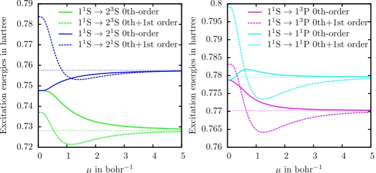
Figure 2. Zeroth-order (plain line) excitation energies ∆Ekµ =Ekµ− E0µand zeroth+first-order (dashed line) excitation energies ∆Ekµ,(0+1)=Ekµ,(0+1)−E0µ,(0+1)(in hartree) of the helium atom as a function ofµ(in bohr−1). The excitation energies of the physical system ∆E
k=Ek−E0are plotted as horizontal
dotted lines.
energies [53] vanishes for the zeroth+first order total energies, which instead depend on the the third power ofµfor smallµ(cf. Eq. (18)). At largeµ, the error relative to the physical energies enters as 1/µ4rather than as 1/µ2in the zeroth-order case,
explaining the observed faster convergence of the first-order energies.
The excitation energies of the helium atom correct to zeroth and first orders are plotted in Figure 2. As previously noted, at µ= 0, the degeneracy of the zeroth-order singlet and triplet excitation energies is lifted by the first-zeroth-order correction. However, the excitation energies correct to first order overestimate the physical excitation energies by 0.1–0.2 hartree so that the error is actually larger than at zeroth order. For the 11S→13P excitation energy, the correction is even going in
the wrong direction and the singlet–triplet splitting is too large by about a factor 1.5.
[image:9.595.94.468.47.222.2] [image:9.595.94.466.274.445.2]Asµincreases further so that more interaction is included, the excitation energies converge toward their fully interacting values from below. The zeroth-order exci-tation energies, which do not oscillate for smallµ, converge monotonically toward their physical limit and are on average more accurate than the zeroth+first order excitation energies. In short, the first-order correction does not improve excitation energies, although total energies are improved.
The inability of the first-order correction to improve excitation energies should be connected to the fact that, since the ground-state density is not kept constant at each order in the perturbation, the ionization potential is no longer constant to first order along the adiabatic connection. This behavior results in an unbalanced treatment of the ground and excited states. Moreover, high-energy Rydberg excita-tion energies should be even more sensitive to this effect, as observed for transiexcita-tions to the P state. The second GL-based variant of perturbation theory should correct this behavior by keeping the density constant at each order, as shown in the KS case [41, 45].
4.2. Beryllium atom
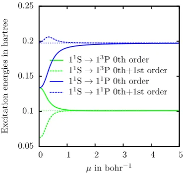
When the first-order perturbation correction is applied to the ground-state and valence-excited states of beryllium, total energies are again improved (not illus-trated here). In Figure 3, we have plotted the zeroth- and first-order valence exci-tation energies of beryllium against the range-separation parameterµ.
Since valence excitation energies should be less sensitive to a poor description of the ionization energy than Rydberg excitation energies, the first-order correction should work better for the beryllium valence excitations than for the helium Ry-dberg excitations. However, although the singlet excitation energy of beryllium is improved atµ= 0 at first order, the corresponding triplet excitation energy is not. In fact, whereas the triplet excitation energy is overestimated at zeroth order, it is underestimated by about the same amount at first order.
As the interaction is switched on, a bump is observed for smallµ for the singlet excitation energy but not the triplet excitation energy, which converges monoton-ically to its physical limit. The convergence of the excitation energies with µ is improved by the first-order excitation energies, especially in the singlet case.
0.05 0.1 0.15 0.2 0.25
0 1 2 3 4 5
µin bohr−1
E
x
ci
tat
ion
en
er
gi
es
in
h
ar
tr
ee
11S→13P 0th order
11S→13P 0th+1st order
11S
→11P 0th order
11S
→11P 0th+1st order
Figure 3. Valence excitation energies of the beryllium atom (in hartree) at zeroth order ∆Ekµ(plain line) and zeroth+first order ∆Ekµ,(0+1)(dashed line), as a function ofµ(in bohr−1). The excitation energies of
[image:10.595.186.371.516.691.2]0.36 0.38 0.4 0.42 0.44 0.46 0.48 0.5
0 1 2 3 4 5
µin bohr−1
E x ci tat ion en er gi es in h ar tr ee
11Σ+
g →13Σ+u 0th order
11Σ+
g →13Σ+u 0th+1st order
11Σ+
g →11Σ+u 0th order
11Σ+
g →11Σ+u 0th+1st order
-0.1 0 0.1 0.2 0.3
0 1 2 3 4 5
µin bohr−1
E x ci tat ion en er gi es in h ar tr ee
11Σ+
g →13Σ+u
11Σ+
g →13Σ+u
11Σ+
g →11Σ+u
11Σ+
g →11Σ+u
11Σ+
g →23Σ+g(σu+)2
11Σ+
g →23Σ+g(σu+)2
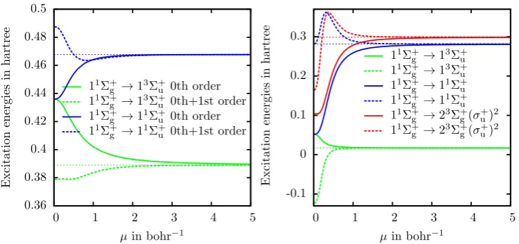
Figure 4. Zeroth-order ∆Ekµ(plain line) and zeroth+first-order ∆Ekµ,(0+1)(dashed line) excitation ener-gies of the hydrogen molecule (in hartree) as a function ofµin bohr−1 at the equilibrium distance (left) and three times the equilibrium distance (right). The excitation energies of the physical system ∆Ekare plotted as horizontal dotted lines.
4.3. Hydrogen molecule
In Figure 4, we have plotted the excitation energies of H2 as a function ofµat the
equilibrium distanceReq and at 3Req. At the equilibrium geometry, the first-order
correction works well. At µ = 0, the correction is in the right direction (singlet and triplet excitation energies being raised and lowered, respectively); for nearly allµ >0, the error is smaller than for the zeroth-order excitation energies.
Unfortunately, when the bond is stretched, this is no longer the case. At the stretched geometry, the first excitation energy 11Σ+
g → 13Σ+u becomes negative
for small values of µ and the error with respect to the physical excitation energy is higher than in the zeroth-order case. Moreover, the ordering of the two singlet excitation energies is incorrect at smallµand they exhibit strong oscillation when the interaction is switched on. In this case, therefore, the zeroth-order excitation energies are better approximations to the physical excitation energies.
5. Conclusion
We have considered two variants of perturbation theory along a range-separated adiabatic connection. The first and simpler variant, based on the usual Rayleigh– Schr¨odinger perturbation theory, was tested on the helium and beryllium atoms and on the hydrogen molecule at equilibrium and stretched geometries. Although total energies are improved to first order in the perturbation, excitation energies are not improved since the theory does not keep the density constant along the adiabatic connection at each order of perturbation. It would be interesting to examine the evolution of the ionization potential to understand better the effect of this variant of the perturbation theory on our systems of interest.
The second variant of the perturbation theory, based on G¨orling–Levy theory, should improve the results significantly by keeping the ground-state density con-stant at each order in the perturbation [41], as already observed on the KS sys-tem [45]. However, this more complicated theory has not yet been implemented for µ >0.
[image:11.595.93.467.46.222.2]system at a givenµ and its first- or higher-order derivatives with respect toµ [72, 73]. Work using this approach will be presented elsewhere.
Acknowledgements
This work was supported by the Norwegian Research Council through the CoE Cen-tre for Theoretical and Computational Chemistry (CTCC) Grant No. 179568/V30 and and through the European Research Council under the European Union Sev-enth Framework Program through the Advanced Grant ABACUS, ERC Grant Agreement No. 267683.
References
[1] M. E. Casida, J. Mol. Struct. THEOCHEM914, 3 (2009).
[2] M. E. Casida and M. Huix-Rotllant, Annu. Rev. Phys. Chem.63, 287 (2012).
[3] O. Gritsenko, S. V. Gisbergen, A. G¨orling, and E. J. Baerends, J. Chem. Phys.113, 8478 (2000).
[4] N. T. Maitra, F. Zhang, R. J. Cave, and K. Burke, J. Chem. Phys.120, 5932 (2004). [5] M. E. Casida, C. Jamorski, K. C. Casida, and D. R. Salahub, J. Chem. Phys. 108, 4439
(1998).
[6] A. Dreuw, J. L. Weisman, and M. Head-Gordon, J. Chem. Phys.119, 2943 (2003). [7] P. Hohenberg and W. Kohn, Phys. Rev136, B834 (1964).
[8] A. Theophilou, J. Phys. C Solid State Phys.5419(1979).
[9] E. K. U. Gross, L. N. Oliveira, and W. Kohn, Phys. Rev. A 37, 2809 (1988). [10] E. Pastorczak, N. I. Gidopoulos, and K. Pernal, Phys. Rev. A87, 62501 (2013). [11] O. Franck and E. Fromager, Mol. Phys.112, 1684 (2014).
[12] Z.-H. Yang, J. Trail, and A. Pribram-Jones, arXiv Prepr. arXiv1402.3209 (2014),
arXiv:1402.3209v1.
[13] A. Pribram-Jones, Z.-H. Yang, J. Trail, K. Burke, R. J. Needs, and C. A. Ullrich, J. Chem. Phys.140, 18A541 (2014).
[14] O. Gunnarsson and B. I. Lundqvist, Phys. Rev. B13, 4274 (1976). [15] T. Ziegler, A. Rauk, and E. Baerends, Theor. Chim. Acta271, 261 (1977). [16] U. von Barth, Phys. Rev. A20(1979).
[17] T. Kowalczyk, S. R. Yorst, and T. Van Voorhis, J. Chem. Phys.134, 54128 (2011). [18] N. Ferr´e and X. Assfeld, J. Chem. Phys.117, 4119 (2002).
[19] M. Krykunov and T. Ziegler, J. Chem. Theory Comput.9, 2761 (2013).
[20] F. A. Evangelista, P. Shushkov, and J. C. Tully, J. Phys. Chem. A117, 7378 (2013). [21] A. Nagy, Int. J. Quantum Chem.70, 681 (1998).
[22] A. G¨orling, Phys. Rev. A59, 3359 (1999).
[23] M. Levy and A. Nagy, Phys. Rev. Lett.83, 4361 (1999). [24] A. G¨orling, Phys. Rev. Lett.85, 4229 (2000).
[25] A. Nagy and M. Levy, Phys. Rev. A63, 52502 (2001). [26] A. Nagy, Int. J. Quantum Chem.99, 256 (2004). [27] M. Harbola, Phys. Rev. A69, 042512 (2004).
[28] V. Vitale, F. Della Salla, and A. G¨orling, J. Chem. Phys.122, 244102 (2005). [29] A. G¨orling, J. Chem. Phys.123, 62203 (2005).
[30] P. Samal and M. K. Harbola, J. Phys. B39, 4065 (2006).
[31] V. N. Glushkov and M. Levy, J. Chem. Phys.126, 174106 (2007). [32] P. W. Ayers and M. Levy, Phys. Rev. A80, 12508 (2009).
[33] P. W. Ayers, M. Levy, and A. Nagy, Phys. Rev. A85, 42518 (2012).
[34] M. K. Harbola, M. Hemanadhan, M. Shamim, and P. Samal, J. Phys. Conf. Ser.388, 012011 (2012).
[35] S. Grimme, Chem. Phys. Lett.259, 128 (1996).
[36] S. Grimme and M. Waletzke, J. Chem. Phys.111, 5645 (1999).
[37] E. V. Beck, E. A. Stahlberg, L. W. Burggraf, and J.-P. Blaudeau, Chem. Phys. 349, 158 (2008).
[40] A. G¨orling and M. Levy, Phys. Rev. B47, 13105 (1993). [41] A. G¨orling and M. Levy, Int. J. Quantum Chem.08, 93 (1995).
[42] A. Savin, C. J. Umrigar, and X. Gonze, Chem. Phys. Lett.288, 391 (1998).
[43] E. J. Baerends, O. V. Gritsenko, and R. van Meer, Phys. Chem. Chem. Phys. 15, 16408 (2013).
[44] R. V. Meer, O. V. Gritsenko, and E. J. Baerends, J. Chem. Theory Comput.10, 4432 (2014). [45] C. Filippi, C. J. Umrigar, and X. Gonze, J. Chem. Phys.107, 9994 (1997).
[46] F. Zhang and K. Burke, Phys. Rev. A69, 052510 (2004). [47] X. Gonze and M. Scheffler, Phys. Rev. Lett.82, 4416 (1999).
[48] A. Savin, inRecent Dev. Appl. Mod. Density Funct. Theory, edited by J.M. Seminario (El-sevier, Amsterdam, 1996), p. 327.
[49] W. Yang, J. Chem. Phys.109, 10107 (1998).
[50] R. Pollet, F. Colonna, T. Leininger, H. Stoll, H.-J. H.-J. Werner, and A. Savin, Int. J. Quantum Chem.91, 84 (2003).
[51] A. Savin, F. Colonna, and R. Pollet, Int. J. Quantum. Chem.93, 166 (2003). [52] J. Toulouse, F. Colonna, and A. Savin, Phys. Rev. A70, 062505 (2004).
[53] E. Rebolini, J. Toulouse, A. M. Teale, T. Helgaker, and A. Savin, J. Chem. Phys.141, 044123 (2014).
[54] O. Franck, B. Mussard, E. Luppi, and J. Toulouse, basis convergence of range-separated density-functional theory (unpublished).
[55] Y. Tawada, T. Tsuneda, S. Yanagisawa, T. Yanai, and K. Hirao, J. Chem. Phys.120, 8425 (2004).
[56] E. Rebolini, A. Savin, and J. Toulouse, Mol. Phys.111, 1219 (2013).
[57] T. Leininger, H. Stoll, H.-J. Werner, and A. Savin, Chem. Phys. Lett.275, 151 (1997). [58] R. Pollet, A. Savin, T. Leininger, and H. Stoll, J. Chem. Phys.116, 1250 (2002). [59] E. Fromager, J. Toulouse, and H. J. A. Jensen, J. Chem. Phys.126, 074111 (2007). [60] E. Fromager, F. R´eal, P. W˚ahlin, U. Wahlgren, and H. J. A. Jensen, J. Chem. Phys.131,
54107 (2009).
[61] E. Fromager, S. Knecht, and H. J. A. Jensen, J. Chem. Phys.138, 084101 (2013).
[62] E. D. Hedeg˚ard, F. Heiden, S. Knecht, E. Fromager, and H. J. A. Jensen, J. Chem. Phys. 139, 184308 (2013).
[63] E. Fromager, S. Knecht, and H. J. A. Jensen, J. Chem. Phys.138, 84101 (2013). [64] J. Toulouse, P. Gori-Giorgi, and A. Savin, Theor. Chem. Acc.114, 305 (2005). [65] P. Gori-Giorgi and A. Savin, Int. J. Quantum Chem.109, 1950 (2009).
[66] A. Stoyanova, A. M. Teale, J. Toulouse, T. Helgaker, and E. Fromager, J. Chem. Phys.139, 134113 (2013).
[67] S. Paziani, S. Moroni, P. Gori-Giorgi, and G. Bachelet, Phys. Rev. B73, 155111 (2006). [68] C. Angeli, K. L. Bak, V. Bakken, O. Christiansen, R. Cimiraglia, S. Coriani, P. Dahle, E. K.
Dalskov, T. Enevoldsen, B. Fernandez, et al., DALTON, a molecular electronic structure program, Release DALTON2011, URLhttp://daltonprogram.org/.
[69] A. M. Teale, S. Coriani, and T. Helgaker, J. Chem. Phys.130, 104111 (2009). [70] A. M. Teale, S. Coriani, and T. Helgaker, J. Chem. Phys.132, 164115 (2010). [71] A. M. Teale, S. Coriani, and T. Helgaker, J. Chem. Phys.133, 164112 (2010). [72] A. Savin, J. Chem. Phys.134, 214108 (2011).
[73] A. Savin, J. Chem. Phys.140, 18A509 (2014).
[74] J. Toulouse, P. Gori-Giorgi, and A. Savin, Int. J. Quantum Chem.106, 2026 (2006). [75] Y. Cornaton and E. Fromager, Int. J. Quantum Chem.114, 1199 (2014).
[76] M. Levy, Proc. Natl. Acad. Sci. U.S.A.76, 6062 (1979). [77] M. Levy, Phys. Rev. A26, 1200 (1982).
[78] E. H. Lieb, Int. J. Quantum Chem.XXIV, 243 (1983).
Appendix A. Double adiabatic connection with a constant density
We here present a double adiabatic connection, depending on two parameters, that keeps the ground-state density constant. It is the basis for the perturbation theory presented in Section 2.2.2. A different density-fixed double adiabatic connection was considered in Refs. [74, 75].
interaction ˆWee is given by [76–78] F[n] = min
Ψ→nhΨ|
ˆ
T + ˆWee|Ψi=hΨ[n]|Tˆ+ ˆWee|Ψ[n]i, (A1)
We here generalize it to the interaction ˆWeelr,µ+λWˆeesr,µ, where ˆWeelr,µ and ˆWeesr,µ are
long-range and short-range electron–electron interactions, respectively, that depend on both a range-separation parameterµand on a linear parameter λ:
Fµ,λ[n] = min
Ψ→nhΨ|
ˆ
T+ ˆWlr,µ
ee +λWˆeesr,µ|Ψi
=hΨµ,λ[n]|Tˆ+ ˆWeelr,µ+λWˆeesr,µ|Ψµ,λ[n]i.
(A2)
The total universal density functional F[n] is then decomposed into Fµ,λ[n] and
a (µ, λ)-dependent short-range Hartree–exchange–correlation density functional ¯
EHxcsr,µ,λ[n],
F[n] =Fµ,λ[n] + ¯EHxcsr,µ,λ[n], (A3) giving the following expression for the exact ground-state energy of the electronic system
E0 = min Ψ
n
hΨ|Tˆ+ ˆVne+ ˆWeelr,µ+λWˆeesr,µ|Ψi+ ¯E sr,µ,λ
Hxc [nΨ] o
, (A4)
where the minimization is over normalized multi-determinantal wave functions. The Euler–Lagrange equation corresponding to this minimization is
ˆ
Hµ,λ|Ψµ,λ
0 i=E
µ,λ
0 |Ψ
µ,λ
0 i, (A5)
where Ψµ,λ0 and E0µ,λ are the ground-state wave function and energy, respectively,
of the Hamiltonian
ˆ
Hµ,λ= ˆT+ ˆV
ne+ ˆWeelr,µ+λWˆeesr,µ+ ˆV¯ sr,µ,λ
Hxc , (A6)
where
ˆ ¯
VHxcsr,µ,λ =
Z δE¯sr,µ,λ Hxc [n0]
δn(r) ˆn(r) dr (A7) is the short-range Hartree–exchange–correlation potential operator, evaluated at the ground-state density of the physical system at µ and λ, n0(r) =
hΨµ,λ0 |nˆ(r)|Ψµ,λ0 i. The Hamiltonian ˆHµ,λthus sets up a double adiabatic connection
with a constant ground-state density.
The range-separated ground-state DFT formalism of Section 2.1 is recovered in the limit λ = 0. To set up a perturbation theory in λ about 0, we rewrite
ˆ
Hµ,λ of Eq. (A6) as the sum of the noninteracting Hamiltonian ˆHlr,µ = ˆHµ,λ=0
and a perturbation operator. For this purpose, the Hartree–correlation–exchange functional is written as
¯
which defines the new functionalEHxcsr,µ,λ[n]. The Hamiltonian can now be rewritten as
ˆ
Hµ,λ= ˆHlr,µ+λWˆeesr,µ−VˆHxcsr,µ,λ, (A9) where
ˆ
VHxcsr,µ,λ=
Z δEsr,µ,λ Hxc [n0]
δn(r) nˆ(r) dr (A10) is the short-range Hartree–exchange–correlation potential operator associated with EHxcsr,µ,λ[n].
The dependence on λof EHxcsr,µ,λ[n] can be made more explicit. It is easy to show that
EHxcsr,µ,λ[n] =hΨµ,λ[n]|Tˆ+ ˆWeelr,µ+λWˆeesr,µ|Ψµ,λ[n]i − hΨµ,λ=0[n]|Tˆ+ ˆWlr,µ
ee |Ψµ,λ=0[n]i, (A11)
which leads to the following decomposition
EHxcsr,µ,λ[n] =λEHxsr,µ,md[n] +Ecsr,md,µ,λ[n], (A12) where
EHxsr,µ,md[n] =hΨµ,λ=0[n]|Wˆeesr,µ|Ψµ,λ=0[n]i (A13) is a multi-determinantal (md) generalization of the usual short-range Hartree– exchange functional [64–66]. Using the variational property of the wave func-tion Ψµ,λ[n], and for non-degenerate wave functions Ψµ,λ=0[n], the expansion of Ecsr,md,µ,λ[n] inλabout 0 starts at second order:
Ecsr,md,µ,λ[n] =λ2Ecsr,md,µ,(2)[n] +· · · , (A14) as in standard GL perturbation theory [40, 41]. The Hamiltonian of Eq. (A9) can now be rewritten as
ˆ
Hµ,λ= ˆHlr,µ+λWˆsr,µ−Vˆcsr,md,µ,λ, (A15) where the perturbation operator ˆWsr,µ= ˆWsr,µ
ee −VˆHxsr,µ,md and
ˆ
VHxsr,µ,md=
Z δEsr,µ Hx,md[n0]
δn(r) ˆn(r) dr (A16) has been introduced to collect all the linear terms inλ, the remaining perturbation operator
ˆ
Vcsr,md,µ,λ =
Z δEsr,µ,λ c,md [n0]