Three dimensional quantification of soil hydraulic properties using X ray computed tomography and image based modeling

(1)

Three dimensional quantification of soil hydraulic properties using X-ray Computed

1 Tomography and image based modelling

2

3 Author list: Saoirse R. Tracy

1$

_{, Keith R. Daly}

2$

_{, Craig J. Sturrock}

1

_{, Neil M. J. Crout}

1

_{, Sacha}

4 J. Mooney

1

_{, Tiina Roose}

2§

5

6 Author affiliations:

7

1

_{School of Biosciences, University of Nottingham, Sutton Bonington Campus, Leicestershire,}

8 LE12 5RD.

9

2

_{Bioengineering Sciences Research Group, Faculty of Engineering and Environment,}

10 University of Southampton, University Road, SO17 1BJ.

11

$

_{These authors are joint lead authors}

12

§

_{Corresponding author: Bioengineering Sciences Research Group, Faculty of Engineering and}

13 Environment, University of Southampton, University Road, SO17 1BJ Southampton, United

14 Kingdom, email: t.roose@soton.ac.uk

15

16 Key Points:

17 

X-ray Computed Tomography is used to image water distribution in soil.

18 

3D Computed Tomography images are combined with image based modelling.

19 

Unsaturated hydraulic conductivity and the water release characteristic are obtained.

20

(2)

1. Abstract

22 We demonstrate the application of a high-resolution X-ray Computed Tomography (CT)

23 method to quantify water distribution in soil pores under successive reductive drying. We focus

24 on the wet end of the water release characteristic (WRC) (0 to -75 kPa) to investigate changes

25 in soil water distribution in contrasting soil textures (sand and clay) and structures (sieved and

26 field structured), to determine the impact of soil structure on hydraulic behaviour. The 3D

27 structure of each soil was obtained from the CT images (at a 10

µm resolution). Stokes

28 equations for flow were solved computationally for each measured structure to estimate

29 hydraulic conductivity. The simulated values obtained compared extremely well with the

30 measured saturated hydraulic conductivity values. By considering different sample sizes we

31 were able to identify that the smallest possible representative sample size which is required to

32 determine a globally valid hydraulic conductivity.

33

34

35

36 Keywords:

Matric potential; soil pores; water release characteristic; X-ray Computed

37 Tomography; image based homogenisation.

38

39 Abbreviations:

40 (3D) - 3-dimensional

41 (CT) - Computed Tomography

42 (ROI) - Region of interest

43

(3)

(WFP) – Water filled pores

45 (AFP) – Air filled pores

46 (REV) -Representative elementary volume

47

48 Short title for page headings: Three

-

dimensional quantification of soil hydraulic properties

49

50

2. Introduction

51 Understanding the dynamic nature of water movement through, and storage within, soil is of

52 fundamental importance for most of its functions. A more detailed knowledge of how soil

53 structure influences soil water distribution and subsequently availability to plants is needed to

54 inform soil management practices and thus contribute to efforts in increasing crop yields for

55 an expanding global population. However, to truly understand how water moves through soil

56 and is retained in soil pores whilst undergoing drying, non-destructive measurements of the

57 soil aggregate geometries and pore structure are needed. The use of X-ray Computed

58 Tomography (CT) to examine the 3D soil pore structure is rapidly gaining pace [

Helliwell

et

59 al.,

2014;

Mooney et al.,

2012]. The ability to segment water from a greyscale CT image

60 remains challenging due to limitations in the phase separation achievable with regular detectors

61 in benchtop CT scanners.

Segmentation of fluids in

alternative

porous media

such as glass

62 beads

has been

previously described

in the literature

[

Haugen et al.

, 2014;

Iassonov et al.

,

63 2009]. However, due to the

more

complex

,

heterogeneous structure of soil and

the associated

64 challenges faced during image acquisition

this brings,

these segmentation techniques cannot

65 always be readily

applied to

the

segmentation of soil

phases

in

X-ray CT

images

[

Houston et

66 al.

, 2013]. Yet, Crestana

et al.

[1985] highlighted the potential of CT for investigating water

67 movement through soil by quantifying the vertical and lateral water flows in 3D. By using dual

68

Deleted:

69

Deleted: well documented

70

Deleted: be easily

71

(4)

energy tomography Rogasik

et al.

[1999] showed it is possible to quantify soil water, pore

73 space and bulk density. Mooney [2002], compared dry and moist samples and developed an

74 imaging method to separate water from the bulk soil in undisturbed soil cores albeit at a

coarse

75 resolution

(0.5 mm)

using a medical CT scanner. Water flow characteristics were

well matched

76 to

macropore structure, with

circa

90% of macropore space active in water transport in a sandy

77 clay texture, compared to

circa

50% in the sandy loam soil. Wildenschild

et al.

[2005]

78 investigated multiphase flow processes and quantified drainage paths show

ing

that water is

79 preferentially lost from larger pores and the drainage of the remaining disconnected pores is

80 prevented. Since then Tippkotter

et al.

[2009] detected soil water in macropores and measured

81 water film thickness at a 20

µ

m resolution. They quantified the water without the use of contrast

82 enhancing agents or comparison of wet and dry scans. Partial volume effects make separating

83 boundaries between phases of interest a challenging task, due to the material of concern often

84 failing to fully fill a voxel [

Ketcham and Carlson

, 2001]. This can lead to individual voxels

85 being misclassified. However, as a microfocus system with a fine resolution was used in the

86 study, the impact of voxel misclassification is minimised [

Clausnitzer and Hopmans

, 2000].

87 The most recent advances in CT imaging technology now allow 3D non-destructive imaging

88 of soils at even higher resolutions,

e.g.

<3

µ

m spot size [

Zappala et al.

, 2013], allowing water

89 to be observed in smaller pores

than previously considered

.

90

91 The macroscopic scale flow in saturated and unsaturated porous media are often described

92 using a Darcy’s law and Richards’ equation [

Hornung

, 1997]. These equations are

93 parameterised by the unsaturated hydraulic conductivity and WRC. From a mathematical

94 perspective Darcy’s law can be derived from the underlying Stokes equations using the method

95 of homogenization [

Keller

, 1980]. This approach has been applied to single porosity materials

96 [

Hornung

, 1997;

Keller

, 1980], double porosity materials [

Arbogast and Lehr

, 2006;

Panfilov

,

97

Deleted: c.circa 0.5 mm

98

Formatted: Font: Not Italic Deleted: similar to

99

Deleted: c.

100

Deleted: c.

101

Deleted: , they

102

Deleted: ed

103

(5)

2000], and porous media containing voids or vugs [

Arbogast and Lehr

, 2006;

Daly and Roose

,

105 2014]. This method is based on the idea that the underlying porous structure is periodic,

i.e.

, it

106 is composed of a set of regular repeating units. By calculating the average fluid velocity for a

107 single representative unit volume due to a unit pressure drop, Darcy’s law and the

108 representative hydraulic conductivity can be derived [

Pavliotis and Stuart

, 2008;

Taylor et al.

,

109 1970]. The mathematics underlying the WRC is less well established and homogenization

110 studies to date have assumed that the air water interface is known in advance [

Taylor et al.

,

111 1970].

112

113 Image based modelling can be loosely divided into two categories: pore network modelling

114 and direct simulation [

Blunt

, 2001;

Blunt et al.

, 2013]. The first of these, pore network

115 modelling, refers to the extraction of a representative network from the pore scale geometry

116 [

Fatt

, 1956] and has been widely used to predict averaged properties of packed spheres [

Bryant

117 and Blunt,

1992;

Bryant et al.,

1993b] and imaged porous media [

Blunt, 2001;

Blunt et al.,

118 2013;

Bryant et al.,

1993a]. This technique is able to reproduce relative permeability curves

119 and water release characteristics. However, the pore network extraction results in a simplified

120 geometry which may neglect important pore scale phenomena. The alternative technique of

121 direct modelling involves solving equations directly on the imaged geometries. This technique

122 captures the detail of the pore scale geometry down to the resolution limit. The key

123 disadvantage is that modelling multiphase flow is demanding from a computational point of

124 view. Typically models of this type are based on Lattice Boltzman simulations of two fluids as

125 these are highly parallel and relatively easy to implement [

Gao et al.

, 2012;

Ramstad et al.

,

126 2010]. Other image based modelling studies in porous media include 3D image based

127 simulations of nutrient transport [

Keyes et al.

, 2013] and saturation based flow modelling of

128

(6)

130 In this paper we demonstrate the application of a high resolution CT method to quantify water

131 distribution in soil pores under successive reductive drying. Using the structural geometries

132 from the CT images we apply the method of homogenization combined with direct image based

133 modelling to calculate the hydraulic conductivity across a range of matric potentials. This can

134 be seen as analogous to the measurement of a wetting phase relative permeability curve.

135 Specifically the question we aimed to answer is: what is the smallest possible Representative

136 Elementary Volume (REV) required to determine a hydraulic conductivity approximation

137 which is globally valid? In addition the soil moisture content is calculated directly from the CT

138 images at a range of different matric potentials and, hence, the WRC is derived. This approach

139 is chosen, rather than Lattice Boltzmann simulation, as it allows the WRC and hydraulic

140 conductivity to be calculated quickly without the need for time consuming two fluid

141 simulations. From the images we are able to obtain information on soil drainage in both

142 undisturbed field cores and sieved soils. This was used to accurately determine the impact of

143 soil structure on hydraulic behaviour.

144

145

3. Materials and Methods

146

147

3.1. Sample preparation

148 Soil was obtained from The University of Nottingham farm at Bunny, Nottinghamshire, UK

149 (52.52° N, 1.07° W). The soils used in this study were a Eutric Cambisol (Newport series,

150 loamy sand/sandy loam) and an Argillic Pelosol (Worcester series, clay loam). Particle size

151 analysis for the two soils was: 83% sand, 13% clay, 4% silt for the Newport series and 36%

152 sand, 33% clay, 31% silt for the Worcester series. Typical organic matter contents were 2.3%

153

Deleted: ¶

(7)

for the Newport series and 5.5% for the Worcester series [

Mooney and Morris, 2008

]. From

155 herein the two soil types are referred to as sand and clay soil. Loose soil was collected from

156 each site in sample bags and field cores (10 mm height, 10 mm diameter) were collected from

157 the immediate soil surfaces after any residues had been cleared. Four replicates were collected

158 for each soil type. Saturated hydraulic conductivity measurements of the field cores were

159 obtained via the standard laboratory method using a constant head device [

Rowell

, 1994].

160 Experimentally obtained hydraulic conductivity measurements were made for comparison with

161 the calculated values.

162

163

3.2. Measurement of the soil water release characteristic

164 In order to investigate the effect of drying on soil water distribution and soil structural changes

165 in 3D, a custom-built tension table was designed to hold the soil sample at a given matric

166 potential, whilst undergoing CT scanning. A small vacuum chamber was constructed

167 (Supplementary Figure 1), that contained a porous ceramic plate (Soil Moisture Corp, Santa

168 Barbara, CA, U.S.A) on top of which a field soil core was placed, with kaolin clay at the base

169 to ensure a good contact. The sample size was kept small to ensure high resolution scanning

170 based on the sample size:resolution trade off that limits CT studies [

Wildenschild et al.

, 2002].

171 The porous ceramic was first submerged in de-aired deionized water and a vacuum applied to

172 ensure no air bubbles remain trapped within the ceramic. The plastic chamber had an O-ring

173 seal at the base and a flange, which was screwed together to ensure an air-tight fit. All

174 components of the chamber were made from plastic to avoid possible image artefacts, which

175 could result from using high X-ray attenuating construction materials such as metal. A 0387

176 Millipore vacuum pump (Merck Millipore, MA, USA) was attached to the chamber and the

177 soil columns were initially saturated from below with deionized water before being

placed

178

179

Deleted:

(8)

under a vacuum of -5 kPa (50.8 mmHg), -10 kPa (76.2 mmHg), -20 kPa (152.4 mmHg), -40

181 kPa (304.8 mmHg), -60 kPa (457.2 mmHg) and -75 kPa (533.4 mmHg).

It was not possible to

182 achieve

pressures in excess of -75 kPa in the system described. The vacuum pump was

enabled

183 for 120 min then the valve sealed to retain the vacuum inside the chamber. At each matric

184 potential the soil core inside the chamber was scanned (further details in next section). After

185 each scan the soil core was removed from the chamber and weighed to calculate gravimetric

186 water content.

187

188 Using a combination of sand tables, pressure plates and pressure membrane apparatus, the

189 WRC were obtained for both soil types. Using conventional methods the van Genuchten model

190 [

van Genuchten

, 1980] was fitted to the data. The sand table was prepared by filling the water

191

[image:8.595.27.575.91.735.2]

reservoir and raising it above the base height of the table to ensure full saturation of the sand

192 table with no air bubbles. Both undisturbed field cores and sieved samples (packed to a bulk

193 density of 1.2 g cm

-3

₎

_{were placed flat on the sand table. To obtain the mid-range points on the}

194 WRC, a pressure plate Model 1600 Pressure Plate Extractor (Soil Moisture Corp, Santa

195 Barbara, CA, U.S.A) was used. Samples were placed on the plate and the samples were

196 weighed frequently until equilibrating at a series of matric potentials. To obtain measurements

197 at lower matric potentials, a pressure membrane apparatus was used. For the sieved samples

198 the required mass of soil was carefully placed into the metal vessels of the pressure membrane

199 apparatus and saturated with air-free water. The field core samples were directly collected in

200 the metal cores and placed onto the apparatus. The collection tubes were weighed frequently

201 and once equilibrated the system was adjusted to higher pressures. After the final measurement,

202 soil samples were oven dried at 105

º

_{C for 24 hr then weighed.}

203

204

Deleted: Despite testing

205

Deleted: , further

206

Deleted: were not possible

207

(9)

The measured volumetric water content of the field structured soil cores (

𝜃

), accounted for the

209 likely presence of stones and their overall influence on the WRC [

Gardner

, 1965;

Reinhart

,

210 1961]. The volumetric water content of the soil is written as

𝜃

which is measured in

cm

3_(H 2O)

cm3_(Soil)

.

211 To calculate this a correction was applied to the measured volumetric water content of the

212 sample,

𝜃

𝑚

, which is measured as

cm

3_(H 2O)

cm3_(Total)

. This stone correction was calculated using

213 𝜃 = 𝜃

𝑚

(1 +

_𝑉𝑉𝑠

𝑓

)

,

(1)

where

𝑉

𝑓

is the fine soil volume measured in

cm

3

(soil)

and

𝑉

𝑠

is the volume of stones which

214 is measured in

cm

3

(stones)

and calculated by subtracting the soil volume from the total

215 sample volume.

216

217

3.3. X-ray Computed Tomography and analysis

218 Four replicates from each soil type of the field cores were scanned at the seven matric potentials

219 giving a total of 56 scans for the field structured cores. As they would not be used for individual

220 pore characterisation analysis only three replicates were scanned for the sieved soils

leading to

221 42 additional scans and a total overall number of 98 scans. The field of view for each scan

222 included the entire sample and each scanned sample created a dataset approximately 25

223 gigabytes in size, which includes all the associated image stacks for analysis,

therefore

2.4

224 terabytes of data was collected. X-ray CT scanning was performed using a Phoenix Nanotom

225 180NF (GE Sensing & Inspection Technologies GmbH, Wunstorf, Germany). The scanner

226 consisted of a 180 kV nanofocus X-ray tube fitted with a diamond transmission target and a

5-227

megapixel (2316 x 2316 pixels, 50 x 50

µ

m pixel size) flat panel detector (Hamamatsu

228 Photonics KK, Shizuoka, Japan). A maximum X-ray energy of 100 kV and 140

µ

A was used

229

Deleted: giving a total of

230

(10)

to scan each soil core. A total of 1440 projection images were acquired over a 360



rotation.

232 Each projection was the average of 3 images acquired with a detector exposure time of 1 s.

233 The resulting isotropic voxel edge length was 10.17

µ

m and total scan time was 105 minutes

234 per core. Although much faster scan times are possible it was necessary in this instance to use

235 a longer scan time to acquire the highest quality images to aid with the phase separation. Two

236 small aluminium and copper reference objects (< 1 mm

2

_{) were attached to the side of the soil}

237 core to assist with image calibration and alignment during image analysis. Reconstruction of

238 the projection images to produce 3D volumetric data sets was performed using the software

239 datos|rec (GE Sensing & Inspection Technologies GmbH, Wunstorf, Germany).

240

241 The reconstructed CT volumes were visualised and quantified using VG StudioMAX

®

_2.2

242 (Volume Graphics GmbH, Heidelberg, Germany). Air, soil and water phases of the scanned

243 volume were segmented separately using a threshold technique based on the greyscale value

244 of each voxel using a calibration tool within VG StudioMax v2.2. This works by selecting

245 specific areas of the scanned volume based on greyscale values, which are a result of (X-ray

246 attenuation) density differences within the sample. Image segmentation is the classification of

247 voxels within a CT volume that share common grayscale values and thus X-ray attenuation.

248 The calibration tool allows the user to sample the greyscale value of a selection of voxels that

249 correspond to the background (

e.g.

the phase/s not considered, this is usually the background

250 air) and then the process is repeated for voxels that correspond to the material of interest (

e.g.

251 water, air or soil). Based on the greyscale range we segmented all voxels above a 50% mean

252 value between the background and material of interest and define them as a particular phase

253 (i.e. a region of interest). In a two phase sample air is usually used as the background greyscale

254 value to calibrate against. However, as we required the segmentation of three phases, two

(11)

vessels, one containing soil pore water and the other finely sieved soil (< 100

µ

m) for either

257 the sand or clay soil were securely fitted to the inside of the chamber

for each scan

. The soil

258 pore water and finely sieved soil remained separate from the soil core, but within the imaging

259 field of view, which was important as the soil core sample can change in overall greyscale

260 range

over

the course of the experiment due to localised drying and X-ray filament aging. Using

261 this approach these separate vessels were used as reference objects during image analysis. It

262 wa

s important that reference vessels

we

re included in every scan as CT scanning is subject to

263 minor variations in greyscales between scans as the system filament ages. A schematic

264 representation of the water segmentation method is presented in Supplementary Figure 2. The

265 first stage was to create a region of interest (ROI) that included

all phases except

the air filled

266 pore space. This was done by selecting the air space around the sample as the background,

267 ensuring

all voxels

except th

os

e

of

air would be included as the material of interest and a 3D

268 ROI was then created and labelled ‘Water and soil ROI’

e.g.

air not included. The process was

269 then repeated, but

utilising

the soil inside the reference vessel as a reference value for the solid

270 material. It was used as a reference as it contained limited water and air,

hence

this 3D ROI

271 was labelled ‘Soil’. Subtraction of the ‘Soil ROI’ from the ‘Water and soil ROI’ resulted in a

272 ROI with voxels of grey scale values attributed to ‘soil water only’,

e.g.

the range of voxels

273 remain

ing

after the soil and air ROIs have been subtracted. The volume of the resulting ‘Soil

274 Water’ ROI was validated against the water reference object and traditional methods of

275 determining volumetric water content (weighing). Using this approach we assume all organic

276 matter is classified as ‘soil’. To create an ROI that included

solely

the air filled pore space, the

277 ROI that included

all material except

the air was inverted using the ‘Invert ROI’ function in

278 VG StudioMax software. The volume analyser tool in VG StudioMax was subsequently used

279 to quantify the total volume of the air and water filled pores. Reconstructed volumes for each

280 matric potential were aligned in VG StudioMax using the metal reference objects on the outside

281

Deleted: throughout

282

Deleted: i

283

Deleted: a

284

Deleted: everything, but

285

Deleted: everything else

286

Deleted: was

287

Deleted: used

288

Deleted: that

289

Deleted: just

290

Deleted: everything but

291

Deleted:

292

Deleted: manually

293

(12)

of the sample container. After segmentation of the soil core volumes

,

a cylindrical ROI shape

295 template was used to subtract the surrounding column and air space from the volume to remove

296 the cylinder of soil. This template was used to ensure the same volume was

used

for each

297 sample before analysis. No significant evidence of shrinkage was observed across the range of

298 low matric potentials considered here. We note that when three phases (air water and soil) are

299 present in an image erroneous films of the intermediate phase can often be segmented out

300 between the high and low density phases. In this case erroneous films of water could be

301 introduced through segmentation. However, as thin water films only contribute a total flow

302 proportional to the third power of the film thickness these are not a concern in this study.

303

304 Image stacks of the extracted volumes were exported and subsequently analysed for individual

305 water filled and air filled pore characteristics for the field structured soil only using ImageJ

306 v1.42 (http://rsbweb.nih.gov/ij/) [

Ferreira and Rasband

, 2011]. For 2D analysis objects less

307 than two pixels (twice the resolution) in diameter (0.02 mm) and for 3D analysis objects less

308 than two voxels in each direction (8 x 10

-6

_mm

3

_{) were regarded as}

_potential

_{noise as a}

309 precaution [

Wildenschild et al.

, 2005] and subsequently excluded from the analysis. The BoneJ

310 plugin algorithm [

Doube et al.

, 2010] (http://bonej.org/) in ImageJ software was used to

311 measure discrete individual 3D water filled and air filled pore characteristics namely volume,

312 surface area and thickness (diameter). A voxel is classed as connected to another voxel if it at

313 least touches corner to corner. ImageJ was used to measure the 2D pore shape characteristic

314 ‘circularity’, which is a measure of an object’s similarity to a circle. A value of 1

describes

a

315 perfect circle and as the value decreases

,

the object becomes increasingly elongated. The

316 circularity was determined using

317 𝐶 =

4𝜋(𝐴_(𝑃 𝑝)

𝑝)2, (2)

318

Deleted: cropped

319

Deleted: 20 µm

320

Deleted: 80 µm3

321

Deleted: and subsequently excluded from the analysis

322

Deleted: .

323

Deleted:

-324

Deleted: perfect

325

(13)

where

Ap

is the pore area and

Pp

is the pore perimeter. The water-filled pore image stack was

327 skeletonised and from this the 3D connectivity (the sum of all the thin (1 voxel) pathways that

328 still preserve the connected topology and original shape of the object) of the water-filled pore

329 volume was also calculated.

330

331 In order for the geometries of the water-filled pores to be modelled, surface mesh files (.stl)

332 were required

which

were generated in VG StudioMax v2.2. After segmentation of the soil

333 water phase, a cube shaped ROI template was imported to create identical cubes for the surface

334 mesh generation. Each sample was subsampled, from random initial coordinates, with 6 cubes

335 comprising side lengths of 3.8 mm. The same coordinates were used for different matric

336 potentials of the same sample. Each individual surface mesh file took between 0.5 – 2 hours to

337 generate depending on the complexity of the surface.

338

339

3.4. Modelling

340 The hydraulic conductivity of the soil was calculated using the method of homogenization

341 [

Pavliotis and Stuart

, 2008]. This method allows an average Darcy’s law to be defined which

342 is applicable to the soil column and is parameterised by the pore scale geometry of the soil.

343 The key assumption used was that the hydraulic properties of the soil can be accurately

344 captured by studying a small subsample of the soil [

Fowler

, 1997], this is often referred to as

345 the Representative Elementary Volume (REV). In this paper we were particularly interested in

346 determining the minimum size REV for which the calculated hydraulic conductivity converges

347 to the macroscopic hydraulic conductivity for soil samples of the order of a few millimetres.

348

Moved (insertion) [1]

Deleted: ; these

349

Deleted: ¶

350

Moved up [1]: In order for the geometries of the water-filled pores

351

to be modelled, surface mesh files (.stl) were required; these were

352

generated in VG StudioMax v2.2. After segmentation of the soil

353

water phase, a cube shaped ROI template was imported to create

354

identical cubes for the surface mesh generation. Each sample was

355

subsampled, from random initial coordinates, with 6 cubes

356

comprising side lengths of 3.8 mm. The same coordinates were used

357

for different matric potentials of the same sample. Each individual

358

surface mesh file took between 0.5 – 2 hours to generate depending

359

(14)

This method allowed us to theoretically determine the required sample size for CT analysis of

361 water flow in soil

at

this scale.

362

363 We note that the averaged hydraulic conductivity and WRC calculated

at

this scale are not

364 globally applicable. Rather they describe the average flow rate in soil of this type assuming no

365 large scale features such as cracks

or

larger voids are encountered. In theory these features

366 could be included by deriving an averaged Darcy’s law for each soil type, Stokes’ equations

367 for large void spaces and approximate Darcy’s laws for fractures equation [

Hornung

, 1997].

368 These systems could, in principle, be upscaled to derive averaged Darcy’s laws on a much

369 larger scale. However, in this paper

our focus is

in obtaining an estimate of the hydraulic

370 properties of soils based on their pore structure. Hence, we neglect these larger scale features

371 but emphasise that they could be included through an additional level of upscaling.

372

373 As we are able to segment the air and water separately from the CT images

,

the fluid dynamics

374 can be greatly simplified. Rather than

focusing on

the moving interface between each phase,

375 we consider the relatively slow, flow of water about a fixed interface. The resulting equations

376 are introduced in the appendix. We further simplify the equations by assuming that the

non-377

wetting phase, in this case air, is stationary. This assumption is valid assuming that the air

378 phase is disconnected. If this is not the case then the movement of the air effectively lubricates

379 the movement of water resulting in an increase in the hydraulic conductivity. This approach is

380 valid assuming that the pressure gradients are sufficiently low, such that the interface remains

381 fixed, and that the non-wetting phase is not connected, hence, the trapped non-wetting phase

382 has zero average velocity.

383

Deleted: on

384

Deleted: ¶

385

Deleted: on

386

Deleted: that

387

Deleted: ,

388

Deleted: or regions of different porosity

389

Deleted: we are interested

390

(15)

392 Strictly speaking the theory of homogenization requires the soil structure to be periodic. Clearly

393 for real soil samples this is not the case. This is overcome by enforcing an apparent image

394 based periodicity either by translation or reflection of the CT image (Figure 1). In this paper

395 reflection was chosen as it simplifies the resulting calculations and does not introduce

396 discontinuities in the soil structure. The error induced by enforcing periodicity is that the

397 geometry considered numerically is now fully periodic rather than quazi-periodic and does not

398 truly represent the imaged soil structure. To overcome this, different size REVs were taken

399 from the segmented .stl files, see Figure 1. Specifically, the 6 cubes which were segmented

400 from each scan were of the same volume

𝑉

𝑚

= 54.9 mm

3

, and were assumed to be sufficiently

401 large that the soil properties would have converged. The REVs sampled from the six cubes

402 were of volume

𝑉 = 𝑉

𝑚

/(2

𝑗

)

, where

𝑗

is a positive integer in the range 0 to 10 such that the

403 smallest volume we consider is

0.

053 mm

3

and the largest is

𝑉

𝑚

. As

𝑗

is decreased and, hence,

404 the size of the REV is increased, the relative size of the errors induced by the reflection

405 decreases. Similarly as the REV size increases, the hydraulic properties of the subsample will,

406 in principle, converge to the hydraulic properties of the soil.

407

408 A rigorous analysis of equations governing fluid flow through soil is given in [

Daly and Roose

,

409 2014]. Here we provide a brief description of the theory in the applied context with further

410 details given in the appendix. We consider a sample of soil which is large with respect to the

411 REV size. Specifically if the REV is a small cube with side length

𝐿

𝑦

and the large sample we

412 are interested in has characteristic length

𝐿

𝑥 then we require that the ratio of these two lengths

413 is small,

i.e.

,

𝜖 = 𝐿

𝑦

/𝐿

𝑥

≪ 1

. For typical pore sizes observed in soil

,

the viscous forces

414 dominate [

Fowler

, 1997]. Hence, we may consider the Stokes limit of the Navier-Stokes

415

Deleted: 𝑛

416

Deleted: 𝑛

417

Deleted: 8

418

Deleted: 2

419

(16)

equations where all inertial terms are neglected. Mathematically the macroscopic hydraulic

421 conductivity, which is valid for the whole soil column, is obtained in two steps. First, it

i

s

422 shown, see appendix for details, that pressure variations across the REV of size

𝜖

will induce

423 a water velocity

also

of size

𝜖

. Secondly, a set of equations are derived which allow the

424 pressure driven fluid velocity to be determined based on the soil (Figure 1). Finally, the average

425 velocity over the REV is used to determine a Darcy's law which is independent of

𝜖

. This value

426 is valid for the bulk soil and describes fluid driven by an external pressure gradient, see [

Daly

427 and Roose

, 2014]

428 𝒖 = −𝒦(𝛁𝑝

0

− 𝜌𝑔𝒆̂

𝑧

),

(3)

where

𝜌

is the fluid density (

𝜌 = 10

3

kg m

−3

in the case of water),

𝑔 = 9.8 m s

−2

is the

429 acceleration due to gravity,

𝑝

0

is the applied pressure,

𝒖

is the volume averaged water velocity

430 and

𝒦

is the relative permeability (in the general case a tensor) which has components defined

431 as

432 𝒦

𝑗𝑘

=

𝐿

2𝑦

𝜇

∫ 𝒆̂

𝑗

⋅ 𝝂

𝑘𝑤

𝑑𝑦

𝛺𝑤

.

(4)

Here

𝒆̂

𝑗

, for

𝑗 = 𝑥, 𝑦, 𝑧

is a unit vector in the

𝑗

-th direction and

𝝂

𝑘𝑤

is the local velocity.

433 Assuming that the air velocity is slower than the water velocity then

𝝂

𝑘𝑤

satisfies the cell

434 problem

435 𝜵 ⋅ 𝜎

𝑘𝑤

− 𝜵𝜋

𝑘𝑤

= 𝒆̂

𝑘

,

𝜵 ⋅ 𝝂

𝑘𝑤

= 0,

𝝂

𝑘𝑤

= 0,

𝝂

𝑘𝑤

= 0,

𝒙 ∈ Ω

𝑤

,

𝒙 ∈ Ω

𝑤

,

𝒙 ∈ Γ

𝑠

,

𝒙 ∈ Γ

𝑎𝑤

,

(5a)

(5b)

(5c)

(5d)

Deleted: ’

436

Deleted: unit cell

437

Deleted: only affect the average water

438

(17)

where

𝜎

𝑘𝑤

= (𝜵𝝂

𝑘𝑤

) + (𝜵𝝂

𝑘𝑤

)

𝑇

,

𝜋

𝑘𝑤

is the local pressure correction due to the microscale

440 geometry, the superscript

𝑤

denotes the water phase,

Ω

𝑤

,

Γ

𝑠

and

Γ

aw

denote the water domain,

441 the soil boundary and the air-water interface respectively. Physically this can be thought of as

442 calculating the fluid velocity subject to a unit pressure gradient. As the equations are linear

443 Darcy’s law follows by multiplying the result by the desired pressure gradient.

444

445 Equations (5) were solved numerically on each subsample obtained from the CT images using

446 OpenFOAM, an open source Computational Fluid Dynamics toolbox running on IRIDIS, the

447 High Performance Computing Facility at the University of Southampton. The hydraulic

448 conductivity is then calculated as the average water velocity due to gravity. Results were

449 obtained for each soil sample using the method illustrated in Figure 1. The 6 cube surface

450 meshes, generated from each soil core, were repeatedly sampled to obtain 3D REVs of

451 increasing size. The result is a set of hydraulic conductivity calculations which we expect to

452 converge to the true hydraulic conductivity of the soil, at each point along the WRC, as the

453 sub-volume size is increased.

454

455

3.5. Statistical analysis

456 The results obtained directly from the CT images were analysed by general analysis of

457 variance (ANOVA) containing soil type and matric potential and all possible interactions

458 as explanatory variables using Genstat 15.1 (VSN International, UK).

459

460

(18)

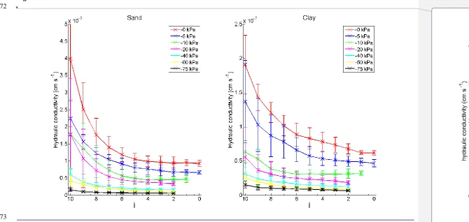
462 4.1 Hydraulic properties

463

464 The clay soil contained an average stone volume of 0.2 cm

3

_{whereas the average stone volume}

465 for the sand soil was 5.5 cm

3

_{(total soil volume was 55 cm}

3

_{). Therefore although field structured}

466 soil was able to retain water for longer, as shown by the curves from the conventional method

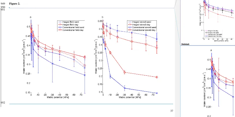
467 (Figure 2)

, the influence of stones

was

not a consideration and the greater water holding

468 capacity is attributed to the more complex pore network in the field structured soil.

469

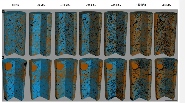
470 There are clear differences between sieved soil and field structured soil (Figures 2 and 3). For

471 the field structured soil the imaging technique shows a good agreement with the conventional

472 methods with an average error of

<

5% across the range of matric potentials considered. The

473 sieved soil responded more strongly to pressure change in comparison to the field structured

474 soil. However, the imaged sieved soil data did not show this trend, hence, there was quite a

475 large error of 9% at 0 kPa and as high as 65% at -75 kPa. This suggests that, for the field

476 structured samples, the segmentation procedure was successful at identifying the majority of

477 the water filled pores (WFPs).

478

479 It is somewhat surprising that the more homogeneous sieved soil is less well represented

480 through the imaging technique than the field structured soil. However,

we

attribute

this

to the

481 pore size distribution in the two soils. The field structured soil

has

a wider range of pore sizes

482 than the sieved soil which contain

s

macropores defined by the largest grain size. As the matric

483 potential

becomes

increasingly negative, the water drains from smaller and smaller pores. In

484

Deleted: samples

485

Deleted: samples

486

Deleted: is

487

Deleted: less than

488

Deleted: this can be

489

Deleted: d

490

Deleted: is likely

491

Deleted: have

492

Deleted: will

493

(19)

the case of the field structured soil this results in a gradual decrease in volumetric water content

495 with matric potential which the imaging technique can follow assuming the pore size is larger

496 than the image resolution. In the case of the sieved soil there is a reduced range of pore sizes

497 and the water quickly drains from the larger pores and remains trapped in a large number of

498 smaller pores. The result is that the volumetric water content drops quickly as the matric

499 potential is reduced and the imaging technique, which cannot resolve the smallest pores, fails

500 to capture this. We also note that the differences observed in the WRC between the two soil

501 types is smaller when measured using the imaging technique than using conventional methods.

502 This is again attributed to the finite resolution of the measurements and is analogous to the

503 increasing error observed as the saturation is decreased.

504

505

506 The hydraulic conductivity, which corresponds to the water release curves shown in Figure 2,

507 has been calculated by solving equations (5) for increasing subsample size. As the subsample

508 size was increased, the hydraulic conductivity converged to a fixed value which we interpret

509 as the macroscopic hydraulic conductivity (Figure 4). The sample size at which this occurred

510 was smaller for lower matric potentials. This is attributed to the increased air-filled porosity

511 which decreases the contact area between the water and the soil. Hence, the effect of the

512 heterogeneous soil boundary is decreased and the overall homogeneity of the sample is

513 increased. We note that, as convergence is seen to occur at smaller sample sizes for lower

514 saturation, fewer simulations were run at these saturation values. This occurs at approximately

515 ¼ of the sample volume for all matric potentials for both soils. We note that although the REV

516 volume is approximately the same for all soil types considered, the properties obtained from

517 this analysis are different for different soil types. This method therefore enabled the required

518

Deleted: the macroscopic

519

(20)

sample size for CT analysis of water flow in these samples to be determined, which was a cube

521 volume of 11 mm

3

_{. This sample was large enough for convergence of the calculated hydraulic}

522 conductivity, meaning that the sample size contained an adequate volume of soil to capture the

523 averaged hydraulic properties on this scale.

Therefore considering

the averaging method used

524 in this paper, the hydraulic conductivity is globally valid. This means that the representative

525 volume of 11 mm

3

_{is an appropriate representative volume element for the global hydraulic}

526 conductivity of the soil samples

used in this study

. However, there may be significant features,

527 such as cracks or heterogeneities in the soil, which are not captured in the 11 mm

3

_volume.

528 Hence, care must be taken in applying these results on the field scale and an additional level of

529 upscaling may be required to capture the properties of these features.

530

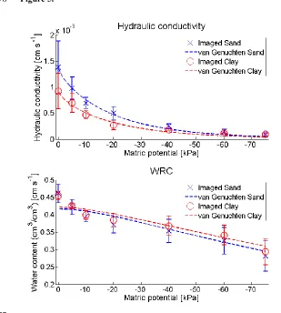
531 The method described in Section 3.4 and the appendix allowed us to also obtain the hydraulic

532 conductivity in unsaturated soils as well as in

x

,

y

and

z

directions. It was expected the flow

533 would be dominant in the

z

direction due to gravity, however (possibly due to the size of the

534 samples) we did not observe this. The calculated hydraulic conductivities are shown as a

535 function of matric potential in Figure 5. The calculated hydraulic conductivities and the

536 corresponding WRC have been fitted to the van Genuchten model for the WRC and the

537 unsaturated hydraulic conductivity [

van Genuchten

, 1980] using a non-linear least squares

538 method. We note that we have only done this fitting for the imaged data as we do not have

539 hydraulic conductivity measurements for the full range of matrix potentials using conventional

540 measurements. The volumetric water content

𝜃

is given by

541 𝜃 = (𝜃

𝑠

− 𝜃

𝑟

) (

_{1 + (𝛼ℎ)}

1

_𝑛

)

𝑚

+ 𝜃

𝑟

,

(6)

Deleted: soil

542

Deleted: We note that, due

543

Deleted: to

544

Deleted: se

545

Deleted: s

546

Deleted: some

547

Deleted: .

548

(21)

where

𝜃

𝑠 and

𝜃

𝑟 are the saturated and residual volumetric water content respectivel

y

,

ℎ

is the

550 is the

matric

head,

𝑚 = 1 − 1/𝑛

and

𝑛

and

𝛼

are the van Genuchten parameters. The

551 corresponding hydraulic conductivity is given by

𝐾 = 𝐾

𝑠𝑎𝑡

𝑘

𝑟𝑣𝑔

. Here

𝐾

𝑠𝑎𝑡

is the saturated

552 hydraulic conductivity and the relative hydraulic conductivity is given by

553 𝑘

𝑟𝑣𝑔

=

{1 − (𝛼ℎ)

𝑛−1

_{[1 + (𝛼ℎ)}

𝑛

_]

−𝑚

_}

2

[1 + (𝛼ℎ)

𝑛

_]

𝑚/2

.

(7)

We take

𝜃

𝑟 to be negligible and fit the remaining parameters to the imaged data. The average

554 saturated hydraulic conductivity and the fitted parameters:

𝐾

𝑠𝑎𝑡

,

𝜃

𝑠

,

𝛼

and

𝑛

are shown in

T

able

555 1. The fitted hydraulic conductivity and WRC, obtained using these parameters, are shown in

556

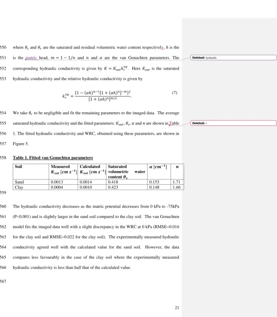
[image:21.595.28.594.67.715.2]

Figure 5.

557 Table 1. Fitted van Genuchten parameters

558 Soil

Measured

𝑲

𝒔𝒂𝒕

[𝒄𝒎 𝒔

−𝟏

]

Calculated

𝑲

𝒔𝒂𝒕

[𝒄𝒎 𝒔

−𝟏

]

Saturated

volumetric

water

content

𝜽

𝒔

𝜶 [𝒄𝒎

−𝟏

_]

_𝒏

Sand

0.0013

0.0014

0.418

0.153

1.71 Clay

0.0004

0.0010

0.423

0.148

1.66

559 The hydraulic conductivity decreases as the matric potential decreases from 0 kPa to -75kPa

560 (P<0.001) and is slightly larger in the sand soil compared to the clay soil. The van Genuchten

561 model fits the imaged data well with a slight discrepancy in the WRC at 0 kPa (RMSE=0.016

562 for the clay soil and RMSE=0.022 for the clay soil). The experimentally measured hydraulic

563 conductivity agreed well with the calculated value for the sand soil. However, the data

564 compares less favourably in the case of the clay soil where the experimentally measured

565 hydraulic conductivity is less than half that of the calculated value.

566

567

Deleted: hydraulic

568

(22)

The differences observed for the clay soil between the experimentally measured hydraulic

570 conductivity and the calculated values are attributed to a combination of image resolution and

571 segmentation

limitations

. Typically clay soils have much smaller pores than sand soils, due to

572 the differences in particle size and as such will have a large number of pores which are

573 comparable with or below the imaging resolution used in this study. Further complications

574 include partial volume effects, which can cause errors in voxel classification, if the boundary

575 is between two phases with wide ranging attenuation values, such as air and rock [

Ketcham

576 and Carlson

, 2001]. This therefore could lead to an incorrect classification of voxels resulting

577 in either an overestimate or an underestimate of the pore space and pore size distribution due

578 to the effect it has on objects of differing sizes

which

may explain why we have an

579 overestimation at the wet end, and underestimation at the dry end. As the calculated hydraulic

580 conductivity is large with respect to the measured value we expect that the pore space is being

581 over estimated in this case.

582

583 4.2 Pore characteristics

584 In order to obtain a better understanding of the pore scale processes which contribute to the

585 macroscopic hydraulic properties we consider the distribution of air and water within the soil

586 matrix on the pore scale. In order to quantify the air and water content we define Air Filled

587 Pores (AFPs) and Water Filled Pores (WFPs) as single connected regions of air or water

588 respectively. We also define the pore space as the union of all the AFPs and WFPs. Throughout

589 this paper when discussing connected regions of water and air we exclusively use this

590 terminology in keeping with the soil science literature. In addition we refer to individual pores

591 within the soil to define simply connected pathways between two distinct points within the

592 pore space. Typically, the pore space contains a single large WFP which contains over 50% of

593

Deleted: , this

594

(23)

the water within the pore space and a large number of much smaller AFPs and WFPs. The

596 connected WFPs are the main contributor to both the WRC and the hydraulic conductivity

597 calculations. However, insight may be gained into the wetting and drying behaviour of the

598 soils by considering the properties of the AFPs. It is possible to determine the interfacial area

599 between water and air phases [

Costanza-Robinson et al.

, 2008]. However, as previous studies

600 have made the calculations based on porous media other than soil, this is not comparable to the

601 work undertaken in this study. In addition the majority of

the previous work in soil

[

Falconer

602 et al.

, 2012;

García-Marco et al.

, 2014;

Tucker

, 2014], refer directly to WFPs and AFPs as

603 such it is more meaningful in the context of the literature to consider the WFP and AFP surface

604 area.

605

606 At 0 kPa we have a residual AFP volume of approximately 6% of the total pore space, see

607 supplementary Figure 3. This volume corresponds to trapped air pockets which, due to the high

608 tortuosity of the soil structure, remain in the pore space at saturation. As the matric potential

609 is made more negative

,

the total WFP volume decreases and the corresponding AFP volume

610 increases (Figure 6; P<0.001). In addition to the change in WFP and AFP volume

,

the total soil

611 volume is seen to increase by up to 10%. Whilst this may, in part, be attributed to segmentation

612 issues

and partial volume effects

,

it is also likely that changes in soil structure are responsible

613 for this apparent increase. The total AFP volume and the corresponding AFP surface area did

614 not vary significantly across the different soil types (sand and clay). However, the average

615 volume and the corresponding surface area of an individual AFP averaged across all matric

616 potentials shows significant variation across soil types (P<0.001) with average AFP volume of

617 0.00115 mm

3

_{in the clay soil compared with}

_{0.00163 mm}

3

_{in the sand soil and with average}

618 AFP surface area of

0.0109 mm

2

in the clay soil and

0.0182 mm

2

in the sand soil. This greater

619 surface area corresponds to a much greater number of AFPs at -75 kPa in the clay soil (104

620

Formatted: Font color: Text 1

Deleted: researchers working in soil science

621

(24)

pores

/mm

3

) than the sand soil (55 pores

/

mm

3

), (P<0.05). The average pore thickness

622 decreased significantly with decreasing matric potential (Figure 7; P<0.001), from an average

623 of 0.030 mm at 0 kPa to 0.026 mm at -75 kPa. There was no significant difference between soil

624 types. At 0 kPa the average pore thickness for the clay soil was 0.027 mm compared to 0.033

625 mm for sand. At -75 kPa the average pore thickness for the clay and the sand soils was just

626 0.026 mm.

627

628 To highlight the differences in the soil types we classify the AFPs as air filled macro (> 100

629 µ

m), air filled meso (30 - 100

µ

m) and air filled micropores (21 – 30

µ

m), see supplementary

630 Figure 4. This classification is based on the pore diameter,

i.e.

the maximum sphere diameter

631 which can fit inside the pore. The air filled micropore range is

limited

by the achievable

632 resolution based on our estimation of image noise (> 2 voxels).

As the matric potential is

633 decreased

,

the total number of AFPs classified into each category changes with an overall

634 increase in the number of air filled macropores seen in the case of the sand soil. In the sand

635 soil there is a linear increase in the percentage of air filled macropores with soil drainage, this

636 was expected due to the high number of macropores throughout the sand structure, which is

637 typically more homogenous compared to the clay. The clay soil had a less regular drainage

638 pattern than the sand soil. There is a linear increase in the air filled micropore percentage as

639 the clay dried. However, the percentage of air filled macropores is quite irregular and can be

640 attributed to the occurrence of crack formation which is more likely in clay soil. The average

641 pore

circularity of the AFPs, equation (2), also increased as matric potential decreased. At -75

642 kPa the AFP space was comprised of pores with an average circularity of 0.78 compared to a

643 circularity value of 0.72 at 0 kPa (P<0.001). Our results also show that at drier matric potentials