Compact objects in active galactic nuclei and X ray binaries

(1)

THE UNIVERSITY OF ST. ANDREWS

Compact Objects in Active Galactic Nuclei and X-ray

Binaries

Edward M. Cackett

Submitted for the degree of Ph.D.

(2)

DECLARATION

I, Edward Cackett, hereby certify that this thesis, which is approximately 50,000 words in length, has been written by me, that it is the record of work carried out by me and that it has not been submitted in any previous application for a higher degree.

Date Signature of candidate

I was admitted as a research student in October 2003 and as a candidate for the degree of Ph.D in October 2004; the higher study for which this is a record was carried out in the University of St Andrews between 2003 and 2006.

(3)

In submitting this thesis to the University of St Andrews I understand that I am giving permission for it to be made available for use in accordance with the regulations of the University Library for the time being in force, subject to any copyright vested in the work not being affected thereby. I also understand that the title and abstract will be published, and that a copy of the work may be made and supplied to any bona fide library or research worker, that my thesis will be electronically accessible for personal or research use, and that the library has the right to migrate my thesis into new electronic forms as required to ensure continued access to the thesis. I have obtained any third-party copyright permissions that may be required in order to allow such access and migration.

Date Signature of candidate

I hereby certify that the candidate has fulfilled the conditions of the Resolution and Reg-ulations appropriate for the degree of Ph.D in the University of St Andrews and that the candidate is qualified to submit this thesis in application for that degree.

(4)

Acknowledgements

First, and foremost, I would like to thank my inspirational supervisors Keith Horne and Rudy Wijnands. Their enthusiasm, help, advice and insight (the list could easily continue) has been paramount to me enjoying astronomy research so much.

The continual love and support of my parents and family throughout my educa-tion has always been much appreciated. Catr´ıona, thank you for your love, support and friendship, it means the world to me.

Thanks also to all my collaborators for insightful, and enjoyable discussions on many aspects of this work, especially Mike Goad, Kirk Korista, Hartmut Winkler, Craig Heinke and Dave Pooley.

I would like to thank Sidney Harris (http://://www.sciencecartoonsplus.com), for kind permission to reprint his cartoons in this thesis.

(5)

Preface

This thesis is based on all the first author papers listed below. Additionally, Chapter 3 will shortly be submitted as a paper to MNRAS.

[1] Cackett, E. M., Wijnands, R., Linares, M., Miller, J. M, Homan, J., Lewin, W. H. G. 2006, MNRAS, 372, 479

[2] Cackett, E. M, Wijnands, R. & Remillard, R. 2006, MNRAS, 369, 1965

[3] Cackett, E. M., Wijnands, R., Heinke, C. O., Edmonds, P. D., Lewin, W. H. G., Pooley, D., Grindlay, J. E., Jonker, P. G., Miller, J. M.

2006, MNRAS, 369, 407

[4] Cackett, E. M., Horne, K. 2006, MNRAS, 365, 1180

[5] Cackett, E. M., Wijnands, R., Heinke, C. O., Edmonds, P. D., Lewin, W. H. G., Pooley, D., Grindlay, J. E., Jonker, P. G., Miller, J. M.

(6)

THE UNIVERSITY OF ST. ANDREWS

Compact Objects in Active Galactic Nuclei and X-ray Binaries

Submitted for the degree of Ph.D.

4 August 2006

Edward M. Cackett

ABSTRACT

In this thesis I study the inner-most regions of Active Galactic Nuclei (AGN) us-ing the reverberation mappus-ing technique, and neutron star low-mass X-ray binaries in quiescence using X-ray observations.

Using the 13-year optical monitoring data for the AGN NGC 5548, the luminosity-dependence of the Hβ emitting radius was modelled using a delay map, finding that the radius scales with luminosity as predicted by recent theoretical models. Time-delays between the continuum at different wavelengths in AGN can be used to probe the accretion disc. Here, continuum time-delays in a sample of 14 AGN were used to measure the radial temperature profile of the accretion discs, determine the nuclear extinction, and measure distances to the objects. However, the distances measured correspond to a value for Hubble’s constant that is a factor of_∼2 lower than the accepted value. The implications of this on the thermal disc reprocessing model are discussed.

(7)

LIST OF FIGURES

1.1 An artist’s impression of an accretion disc around and AGN and in an X-ray

binary system . . . 2

1.2 The UV spectrum of Seyfert 1 galaxy NGC 5548 . . . 5

1.3 Optical continuum and Hβ lightcurves for NGC 5548 . . . 7

1.4 Relativistic iron line profile in MCG₋6₋30₋15 . . . 8

1.5 Unified model of AGN . . . 10

1.6 Iso-delay surfaces . . . 11

1.7 Constraints on ΩM and ΩΛ from SNe Ia observations . . . 20

1.8 The magnitude difference between the distance modulus of 3 different cos-mologies and an empty cosmology . . . 21

1.9 A diagram outlining the structure of a neutron star (not to scale). . . 27

1.10 Optical and X-ray images of the globular cluster 47 Tucanae . . . 29

1.11 Number of globular cluster X-ray sources vs. stellar encounter rate . . . 30

1.12 Design of the Chandra mirrors. . . 36

2.1 Optical continuum and Hβ emission line lightcurves for NGC 5548 . . . 46

2.2 Non-linear response of emission lines to continuum variations . . . 47

2.3 Delay maps for different values of the ‘breathing’ parameters . . . 50

(13)

2.5 τmed vs. mean optical continuum flux for static delay map fit to yearly data 54

2.6 Data and residuals for B2 model fit to the 1989-2001 Hβ lightcurve . . . 56

2.7 Luminosity-dependent delay maps for the 5 parameterized models as well as theMEMECHOrecovered delay map . . . 58

2.8 Continuum and Hβ lightcurves for 1991 - 1992 and 1998 - 1999 with fits to the Hβ lightcurve . . . 59

2.9 MEMECHOfit to optical continuum and Hβemission line lightcurves for NGC 5548 61 2.10 MEMECHOluminosity-dependent delay map for NGC 5548 . . . 62

2.11 10 realisations of the MEMECHOrecovered delay map . . . 62

2.12 A section of the MEMECHOfit to the continuum lightcurve . . . 65

2.13 A comparison of the characteristic shape of the Hβ line profile and the residuals of the B2 fit . . . 66

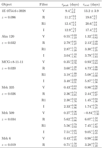
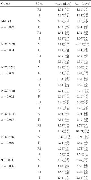
3.1 B-band lightcurves for 14 AGN . . . 74

3.2 Lightcurves for NGC 5548 in all 5 bands, with corresponding CCFs . . . 75

3.3 Lightcurves for NGC 7469 in all 5 bands, with corresponding CCFs . . . 76

3.4 Comparison ofτpk and τcent . . . 77

3.5 Irradiated accretion disc transfer functions . . . 83

3.6 Flux-flux diagrams for NGC 3516 and NGC 7469 . . . 86

3.7 Comparison ofE(B₋V)n determined by the flux-flux and Balmer decre-ment methods . . . 87

3.8 The adopted extinction law of Nandy et al. (1975) and Seaton (1979) eval-uated atE(B₋V) = 1.0. . . 88

3.9 χ2 parabola for the distance to NGC 7469 . . . 89

(14)

3.11 A comparison of the total E(B-V) values determined via the reprocessing

model and the flux-flux and Balmer decrement methods . . . 96

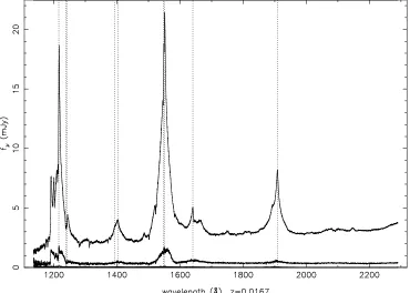
3.12 Optical spectrum of 3C 390.3 . . . 96

3.13 Normalised dereddened galaxy spectra . . . 97

3.14 Hubble diagram for 14 AGN . . . 97

3.15 Residuals compared to AGN properties . . . 101

3.16 Simulation of constraints on H0, ΩM and ΩΛ from 44 AGN . . . 104

3.17 Constraints onH0, ΩM and ΩΛ from 185 supernovae type 1a . . . 105

4.1 RXTE ASM light curve of the transient in NGC 6440 . . . 110

4.2 Chandra X-ray Images of the globular cluster NGC 6440 . . . 111

4.3 X-ray spectra of the X-ray transient neutron star in NGC 6440 during observations 1 and 2 . . . 116

4.4 Comparison of the effective temperature between observations 1 and 2 . . . 117

5.1 Digitized Sky Survey (DSS) image of Terzan 1 . . . 123

5.2 Chandra ACIS-S image of the globular cluster Terzan 1 in the 0.5-8.0 keV energy band . . . 125

5.3 X-ray color magnitude diagram for Terzan 1 . . . 130

5.4 The spectrum of the brightest source in Terzan 1, CXOGLB J173545.6-302900134 6.1 RXTE All-Sky Monitor 7-day averaged lightcurve for KS 1731₋260 and MXB 1659₋29. . . 144

6.2 Cooling curves for KS1731₋260 . . . 151

6.3 Cooling curves for MXB1659₋29. . . 156

(15)

7.2 EPIC-pn 0.2-10 keV background subtracted lightcurve for XMMU J181227.8₋181234166

7.3 EPIC-pn spectrum for XMMU J181227.8₋181234 with best-fitting absorbed multi-colour disk blackbody model . . . 168

7.4 7-day averagedRXTEASM lightcurve for XMMU J181227.8₋181234 . . . 170

7.5 RXTEASM colour-colour diagram . . . 171

(16)

LIST OF TABLES

2.1 Parameters for fits of the Static model to the yearly Hβ lightcurves of NGC

5548 . . . 52

2.2 Parameters for fits to 1989-2001 Hβ lightcurve of NGC 5548 . . . 57

2.3 Time delay at the median, lower and upper quartile of theMEMECHO luminosity-dependent delay map for each continuum flux. . . 60

3.1 Fluxes (in mJy) for the comparison stars . . . 71

3.2 Time-delays relative to the B-band determined by cross-correlation. . . 72

3.3 Maximum and minimum fluxes (mJy) from the AGN lightcurves . . . 77

3.4 Nuclear extinction, E(B ₋V)n, determined by the flux-flux and Balmer decrement methods . . . 87

3.5 Best-fitting parameters from reprocessing model . . . 94

4.1 Spectral results for observation 1 . . . 114

4.2 Spectral results for observation 2 . . . 114

4.3 Spectral results when simultaneously fitting to observations 1 and 2 . . . . 116

5.1 Details of 14 sources detected within 1.04 of the center of Terzan 1 and the sources detected on the rest of the S3 chip . . . 126

(17)

6.1 Details of the Chandra (CXO) and XMM-Newton (XMM) observations of KS 1731₋260. . . 147

6.2 Neutron star atmosphere model fits to the X-ray spectrum of KS 1731₋260 for 5Chandra (CXO) and 3 XMM-Newton(XMM) observations. . . 150

6.3 Details of the Chandra (CXO) and XMM-Newton (XMM) observations of MXB 1659₋29. . . 153

6.4 Neutron star atmosphere model fits to the X-ray spectrum of MXB 1659₋29 for 5Chandra (CXO) and 1 XMM-Newton(XMM) observations . . . 155

(18)

CHAPTER 1

Introduction

(19)

Figure 1.1: An artist’s impression of the an accretion disc around a supermassive black hole in an Active Galactic Nucleus (left), and a stellar-mass black hole in an low-mass X-ray binary (right). While the mass scales are wildly different, the same physical process is thought to be powering both. Credit: NASA/CXC/M.Weiss

Due to the different size scales, the temperatures of accretion discs in binary systems peak in the X-rays, whereas accretion discs in AGN peak in the EUV/UV and have significant emission in the optical (though AGN discs also emit in the X-ray and X-ray binary discs emit in the UV and optical too). The timescales in the two classes of objects are also different, with X-ray binaries varying on much shorter timescales (as fast as milliseconds in some cases as opposed to days in AGN). Studying accretion in both X-ray binaries in our Galaxy and AGN may lead to the scaling of properties with mass between the two. Of course, if we can understand what is going on in one type of system, it could improve our understanding of the other and help to build one coherent picture of accretion in strong fields on all scales.

AGN are some of the most luminous objects in the Universe and can be seen to significant redshifts where the Universe was only a fraction of the age it is now. If AGN can be used as a standard candle, they provide a very attractive way to probe cosmology to high redshifts, much further than can be seen with current supernovae methods.

(20)

ultra-dense matter that makes up these stars.

In this thesis I study the inner-most regions of AGN, and demonstrate the potential of using AGN accretion discs as standard candles to probe cosmology. I also focus on the study of neutron star low-mass X-ray binaries in quiescence and discuss the implications of these observations on the properties of the neutron stars in these systems.

1.1 Active Galactic Nuclei

Active Galactic Nuclei (AGN) refers to the central region of a galaxy, known as the galactic nucleus, that is observed to be particularly energetic, in many cases outshining the rest of the galaxy. In 1943 Carl Seyfert noted that a reasonable proportion (up to a few percent) of spiral galaxies have high central surface brightnesses that are point-like and as bright as the rest of the galaxy (Seyfert, 1943). Radio astronomers in the 1950’s performed large radio surveys of the sky and discovered many AGN. For example, a bright radio source associated with Cygnus A, a galaxy faint in the optical, was found and later revealed to be two huge radio lobes extending to a quarter of a million light years either side of the nucleus to which it is connected by jets (collimated outflows travelling close to the speed of light). Further radio surveys in the 1960’s observed other strong radio signals that were found to come from star-like objects exhibiting strong broad emission lines. Although at the time the nature of these quasi-stellar radio sources, or quasars, was very confusing, we now know them to be the extremely bright centres of galaxies.

While there is a veritable smorgasbord of different AGN subclasses (for example Seyferts, quasars, blazars), they all show most, if not all, of the following properties: nuclei with small angular size (so small that they cannot be spatially resolved), a high luminosity (_∼1042−48 erg s−1), broad-band continuum emission from the radio to hard X-rays, strong optical and UV emission lines, and variability in the continuum and emission lines.

(21)

at which the gravitational force acting on the gas is balanced by the outward force of radiation) for AGN provides a lower limit for the masses of the central supermassive black holes, and indicates they may be around M = 106−9 M¯. This makes the study of AGN particularly important as they are the only place to study black holes on this scale. As AGN are bright, they are seen over a wide range of redshifts and so also provide a way of studying the evolution of supermassive black holes.

1.1.1 Emission Lines

A particular feature of most AGN is their strong emission lines in the optical and UV. A wide number of emission lines are observed, but they can be split into broad lines and narrow lines, where broad lines are those that are seen to have ‘broad’ profiles with widths corresponding to velocities between 103 _{and 10}4 _{km s}−1 _{and narrow lines are those that}

have ‘narrow’ profiles with widths corresponding to velocities of several hundred km s−1. An example of broad emission lines is shown in the UV spectrum of NGC 5548 (Fig. 1.2).

There are many broad emission lines found in AGN spectra but some of the stronger lines include Lyα, Hα, Hβ, HeIIλ1640 and CIVλ1549. Importantly, only permitted broad emission lines are seen. The absence of forbidden broad emission lines indicates that the broad-line gas must exceed a minimum density. In contrast, forbidden narrow emission lines are seen (e.g. [OIII] λ4959,5007, [OII] λ3727, [NII] λ6583, [OI] λ6300, and [SII] λ6724), as well as some permitted narrow emission lines, indicating the gas responsible is

less dense than the broad-line gas.

The mechanism behind the formation of these emission lines is photoionization by the continuum. Evidence for this includes the correlated continuum and emission-line fluctuations (see section 1.2 for more details). Also, in some nearby AGN the narrow-line region is seen to occupy a triangular projection on the sky, known as an ‘ionization cone’ (e.g. Pogge, 1988; Tadhunter & Tsvetanov, 1989). These ionization cones can be explained by photoionization excitation where the ionizing radiation has been collimated close to the nucleus (e.g., Bland-Hawthorn, Cackett and Maloney 2006, in preparation).

(22)

[image:22.595.152.522.203.467.2]

(23)

2 (Khachikian & Weedman, 1974). Type 1 Seyferts have both narrow emission lines and broad emission lines present. However, Seyfert type 2 galaxies do not exhibit broad emission lines and only narrow emission lines are present. The continuum in Seyfert 2’s is also observed to be weaker.

1.1.2 Variability

Variability is a property observed in many AGN on timescales of days to months with little variability seen on timescales shorter than a few days. Variability has been observed in all wavebands, and in the broad emission lines as well as the continuum (see Fig.1.3). The observed rapid variability implies that the size of the continuum-emitting region is of the order of light days - if an object varies with a timescale, t, then the radius of the varying region must beR_≤ct otherwise the light time travel would smooth out the time variations.

Although periodic behaviour has not been identified in AGN variations, the vari-ability can be characterised. For example, one can look at the mean fractional variation, which is typically around 10-20% in the optical continuum on timescales of about a month. Another useful way to characterize the variability is to look at the power-density spec-trum - the product of the Fourier transform of the light curve and its complex conjugate. This indicates the power-density in the variations per unit frequency. AGN are seen to have a broken power-law like power-density spectrum,P(f)_∝f−α_{, typically with} _α_∼₂

above the break frequency and flattening off at low frequencies to α _∼1, with the break frequency seemingly scaled with mass, though other parameters such as the mass accre-tion rate likely provide the large scatter in this relaaccre-tionship (e.g., Markowitz et al., 2003; McHardy et al., 2004, 2005). Optical and UV continuum variability is understood to be due to reprocessing by the accretion disc of varying EUV/X-ray ionizing radiation, whereas the variable broad lines are due to the heating and reprocessing of the ionizing radiation in the broad line gas.

1.1.3 The current AGN paradigm

(24)

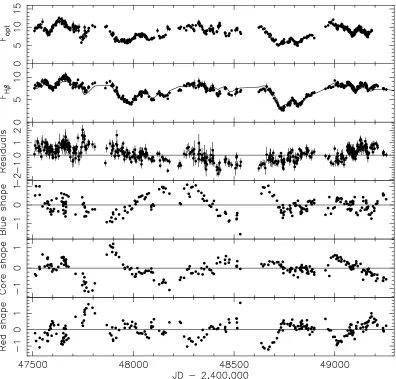
47500 47600 47700 47800 4

6 8 10 12 144 6 8 10

12 NGC 5548

Continuum

Figure 1.3: Optical continuum at 5100 ˚A (bottom panel) and the Hβ (top panel) lightcurves of NGC 5548 from the first year of monitoring by the AGN Watch collab-oration. The continuum fluxes are in units of 10−15 _{ergs s}−1 _cm−2 _˚_A−1 _{and the Hβ} _fluxes

are in units of 10−13 ergs s−1 cm−2 ˚A−1. Data is from AGN Watch NGC 5548 observing campaign (Peterson et al., 2002, and references therein).

are all intrinsically identical with the observed differences explained simply by differing luminosities and/or viewing angles. The basic components of this model are a supermassive black hole and accretion disc, high velocity gas clouds close to the nucleus giving rise to the broad lines, a region of low velocity gas clouds further away from the nucleus giving rise to the narrow lines and a dusty torus that obscures the nucleus from some viewing angles.

(25)

Figure 1.4: Relativistic iron line profile in the AGN MCG₋6₋30₋15 from a 325-ks observation with theXMM-NewtonX-ray telescope. The line has a broadened asymmetric profile with most of the line flux redshifted from its rest energy of 6.4 keV. Taken from Fabian et al. (2002).

water maser emission in NGC 4258 with 0.13 pc of a massive object (Miyoshi et al., 1995) supports the accretion disc idea. Further strong evidence for AGN accretion discs is given by the gravitationally redshifted Fe K-αemission line that has been observed in the X-ray spectra of several AGN (Tanaka et al., 1995). The broad, asymmetric profiles with most of the line flux redshifted indicates that the line arises from a region several Schwarzschild radii from a supermassive black hole. See Fig. 1.4 for an example of the relativistic iron line in the AGN MCG₋6₋30₋15 and Reynolds & Nowak (2003) for a review of this topic.

The broad emission lines have widths corresponding to high velocities and the ab-sence of forbidden broad lines indicates the gas is of high density. This suggests that the broad line region (BLR) must be close into the nucleus (we discuss reverberation mapping observations of the BLR in_§1.3). The narrow line region (NLR) is a lower density, lower velocity gas and is the smallest scale that can be spatially resolved in even the nearest AGNs. The IR emission seems to arise from warm dust grains which must form in a region that is cooler than the dust sublimation temperature.

(26)

for unification is based on the idea that there is obscuration of the nucleus by optically thick dust along some lines of sight. Whether the dust is in a molecular torus (e.g. Krolik & Begelman, 1988; Pier & Krolik, 1992a,b, 1993) or is the outer edges of a warped accretion disc (e.g. Sanders et al., 1989) or something else is unclear, however, it is still generally referred to as being a dusty torus, whatever its nature. Recent deep multiwavelength surveys have discovered a significant population of obscured AGN (where the obscuration is due to a dusty torus) by comparing X-ray and IR observations, as predicted by AGN unification, with 3 times as many obscured AGN as unobscured (Treister et al., 2004, 2006).

The simplistic general unified model is shown in Fig. 1.5. From this it is clear that by changing the viewing angle, one would observe different properties. For instance, if viewing close to edge-on the obscuring dusty torus would prevent the nucleus and BLR from being viewed directly and only the narrow lines would be present in the spectrum, hence the AGN would be classed as a Seyfert 2. Alternatively, viewing close to face-on would allow the nucleus and BLR to be seen and the AGN would be classed as a Seyfert 1. The fact that the continuum is weaker in Seyfert 2’s than in Seyfert 1’s is also explained by the obscuring of the nucleus. Only light from the nucleus scattered or reflected by dust or free electrons reaches an observer that is edge-on. Evidence for this has been seen in the polarized spectrum of the nearby Seyfert 2 galaxy NGC 1068 (Antonucci & Miller, 1985; Miller et al., 1991) and some other nearby Seyfert 2 galaxies (Miller & Goodrich, 1990). In this case, weak broad emission lines have been detected in the polarized spectrum indicating that Seyfert 1 and 2 galaxies are intrinsically identical, in at least a handful of sources.

1.2 Reverberation Mapping

(27)

Jet

Obscuring Torus

Narrow Line Region

Disc Accretion Black

Hole

Broad Line Region

Figure 1.5: Schematic diagram showing the simplistic unified model of AGN. A Seyfert 1 will be observed when viewing close to face-on, whereas when viewing edge-on the dusty torus obscures the nucleus and BLR so a Seyfert 2 is observed. Credit: CXC/M. Weiss

through the disc and gas at the speed of light. The incident ionizing radiation is then absorbed by the gas and reprocessed into emission-line photons. As the reprocessing time is insignificant compared to the light travel time, the light travel time dominates the observed time delay. Changes in the ionizing radiation (peaks or dips in the lightcurve) have the knock-on effect of causing changes in the reprocessed emission at observable time delays. This causes the emission-line light curve to be delayed and smeared compared to the continuum light curve. Reverberation (or ‘echo’) mapping (Blandford & McKee, 1982) uses these observable time delays to indirectly determine information on the kinematics and geometry of the accretion disc and BLR.

1.2.1 Time Delays

(28)

Figure 1.6: Schematic view of the BLR modelled as a thin spherical shell with isodelay paraboloids indicated. The different path length for radiation travelling directly from the compact nucleus to the observer and the radiation that travels to the BLR and then to the observer leads to an observable time delay given byτ =R/c(1 + cosθ) whereRis the radius andθis the azimuth angle measured to be 0◦ _{along the line of site on the far-side} of the nucleus and 180◦ on the near side. At any time, τ the observer sees reprocessed photons at the intersection of an isodelay paraboloid and the BLR.

by:

τ = R

c (1 + cosθ) (1.1)

(29)

1.2.2 Transfer Functions

The most simple linearized model of the emission line light curve,L(t), driven by contin-uum variations,C(t) is given by:

L(t) = ¯L+ Z ∞

0

Ψ(τ)¡

C(t₋τ)₋C¯¢

dτ (1.2)

where ¯C is the background continuum flux, ¯L is the constant background line flux that would be produced if the continuum were constant at ¯Cand Ψ(τ) is the transfer function or delay map. In these 1-dimensional terms, the time delay map, Ψ (τ), is effectively a map of the strength of the emission line region response along the iso-delay surface for time delay, τ. Most analyses of current AGN data have concentrated on solving this 1D case, however, it is possible to use more of the information available to do a 2D analysis. For example, determining a velocity-delay map getting velocity information from the line width (e.g., Horne et al., 1991; Welsh & Horne, 1991; Horne, 1994), or determining a luminosity-delay map to see how the size of the broad-line region changes with luminosity (this is the topic of investigation in Chapter 2).

1.2.3 Techniques for analysing the variability

(30)

Cross-correlation

Cross-correlation is the most commonly used technique, largely because it is easy to im-plement. Cross-correlation of the continuum and emission line light curves is a simple way to determine the mean response time for an individual emission line. It allows a linear shift in time between the two light curves when determining the correlation. The cross correlation function (CCF) is the convolution integral of the line light curve with the continuum light curve (e.g., Peterson, 1993),

CCF(τ) = Z ∞

−∞L(t)C(t−τ) dt . (1.3)

We have previously definedL(t) in Eq. 1.2 which then gives

CCF(τ) = Z ∞

−∞C(t−τ) Z ∞

−∞Ψ(τ 0_)C(t

−τ0) dτ0 dt

= Z ∞

−∞ Ψ(τ0)

Z ∞ −∞

C(t₋τ0)C(t₋τ) dtdτ0 . (1.4)

The autocorrelation function (ACF) is defined as being the cross-correlation of the con-tinuum light curve with itself, i.e.,

ACF(τ) = Z ∞

−∞C(t)C(t−τ) dt . (1.5)

It is then possible to write the CCF in terms of the convolution integral of the delay map with the continuum ACF,

CCF(τ) = Z ∞

−∞

Ψ(τ0)ACF(τ ₋τ0) dτ0 (1.6)

Thus, the time-delay, or ‘lag’, for a particular emission line is just given by the peak or centroid of the CCF. Importantly, the lag measured depends not only on the delay-map but also on the nature of the continuum lightcurve, given by the ACF. The lag will occur at the mean time delay for the system, i.e. atτ =R/c for a thin spherical shell of radius R or a thin ring of radius R. Thus, from the time-delay, the size of the BLR can be determined.

(31)

Interpolation Method

We use the interpolation method in the modified version of Gaskell & Peterson (1987) by White & Peterson (1994). In this method each emission line data point, L(ti), is paired

with a linearly interpolated continuum value at C(ti−τ) and the CCF determined for a

wide range of time delays,τ using:

CCF(τ) = 1 N

N

X

i=1

[L(ti)−L][C(t¯ i−τ)−C]¯

σcσL

, (1.7)

where there are N data points, ¯L and σL are the mean and standard deviation of the

emission line flux data points,L(ti), and ¯C andσC are the mean and standard deviation

of the continuum flux data points,C(ti). All points outside the time series (ti−τ < t1 or

ti−τ > tN) are excluded. This is then repeated but pairing the continuum data points,

C(ti), with linearly interpolated emission line values at L(ti+τ) and the average of the

two cross-correlation functions taken. The advantage of the interpolation method is that it can give results from just a few data points. However, if the interpolation of the data points is not a good representation of the true light curve the results can be misleading and thus a well-sampled lightcurve is required.

1.3 Previous Observational Results

1.3.1 Size and Radial Structure of the BLR

Previous observations have focused on determining the size of the BLR by measuring the lags of different emission lines compared to the continuum. The International AGN Watch1collaboration undertook a 13-year ground based campaign for the Seyfert 1 galaxy NGC 5548, one of the best studied AGN (see Peterson et al., 2002, and references therein) as well as obtaining UV data with IUE and HST (Korista et al., 1995). The typical time delay between the continuum and the Hβ emission line is found to be around 20 days, indicating that the distance from the central source that the Hβ line response is most significant is around 20 light days. This collaboration also monitored the variability in other AGNs in the UV and optical (see the AGN Watch webpage for references and further

1_{See http://www.astronomy.ohio-state.edu/}

∼agnwatch for more information on the International AGN

(32)

details). Kaspi et al. (2000) obtained lags for several dozen Seyfert 1s and low-luminosity quasars, as did Wandel et al. (1999). These observations made several important findings. Firstly, the continuum emission in the UV and optical were found to vary with a lag of only a couple of days (see Continuum Variability section below for a discussion). Secondly, it was found that the highest ionization emission lines have the shortest time delays and largest Doppler widths. This implies that there is ionization stratification in the BLR, as expected for ionization by the continuum emission.

The 13-year campaign of NGC 5548 also allows the study of time delay with changing luminosity. As the luminosity increases, one would expect the region that is ionized to increase in size and hence the time delay increase. It is seen that the emission line lag is longer when the continuum source is brighter (Peterson et al., 2002). In Chapter 2 we model this change in size in terms of a luminosity-delay map.

A recent monitoring campaign of a handful of Seyfert galaxies by the MAGNUM collaboration (Suganuma et al., 2004; Minezaki et al., 2004; Suganuma et al., 2006) in the optical and near-infrared wavebands has found lags between the optical V and near-IR K lightcurves ranging from around 10 to 90 days. Other monitoring by Glass (2004) has found lags between the optical and IR of tens to hundreds of days also. These lags are interpreted as thermal dust reverberation from the inner edge of the dusty torus. From these results it appears that the size of the inner edge of the dust torus is well outside the size of the BLR determined by the optical/UV emission line lags for each of the objects.

1.3.2 Black Hole Masses

The mass of supermassive black holes in the cores of many normal galaxies have been determined using stellar dynamics (e.g., Kormendy & Richstone, 1995) and Miyoshi et al. (1995) determined the mass of the central object in Seyfert galaxy NGC 4258 by observing the line-of-sight velocities for water masers in the central regions of the galaxy. Rever-beration mapping also provides a method for determining the black hole mass. Assuming that the velocities of the line-emitting gas are dominated by gravity, the size (from time delays) and velocity (from line widths) can be combined to estimate the mass. From the virial theorem,

M = f r σ

2

(33)

= f τ c σ

2

G (1.8)

where,f is a dimensionless factor of order unity that depends on the geometry and kine-matics of the BLR, σ is the emission line velocity dispersion and r = τ c is the size of the emitting region using the time delay, τ, and speed of light, c. The virial hypothesis predicts that lines formed at different radii in the same object should followτ _∝σ−2, and this anti-correlation is seen (Peterson & Wandel, 1999, 2000; Onken & Peterson, 2002; Kol-latschny, 2003), providing evidence that these reverberation based masses are reasonably accurate measurement of the black hole mass. It has also been found that mass estimates using different emission lines in the same object are consistent with each other (Peterson & Wandel, 1999, 2000), again supporting the accuracy of the mass estimates. Additionally, the relationship between the central black hole mass and the velocity dispersion in the bulge (the so-calledM₋σ relation, Ferrarese & Merritt, 2000; Gebhardt et al., 2000) that was found in quiescent galaxies is seen to hold for AGN (see Onken et al., 2003, 2004, and references therein). Using reverberation mapping, masses ranging from 106 _{to 10}9

M¯ have been determined for many AGNs (e.g., Wandel et al., 1999; Kaspi et al., 2000; Peterson, 2004; Peterson et al., 2004, 2005).

The masses determined by reverberation mapping have been used to calibrate the radius-luminosity relationship where the radius of the broad line region increases with luminosity like R _∝ L0.5 (Kaspi et al., 2000, 2005; Bentz et al., 2006). This important relationship has been used to determine the mass of a black hole from a single measurement of luminosity and line width, allowing mass estimations for large populations of AGN (Wandel et al., 1999; Vestergaard, 2002, 2004; McLure & Jarvis, 2002; Vestergaard & Peterson, 2006).

1.4 Continuum Variability

(34)

Peterson et al., 1998). This suggests that the continuum variations cannot be due to disc instabilities or variable accretion rate as time delays of the order of hundreds of days (i.e. on the viscous timescale) would be expected for these models. It has been proposed that the continuum flux variations are due to reprocessing of variable high-energy (soft X-ray/ EUV) flux (Collin-Souffrin, 1991; Krolik et al., 1991; Clavel et al., 1992). In fact, Krolik et al. (1991) note that as the variations in optical and UV fluxes are almost simultaneous this would require a radial speed for temperature fluctuations within the accretion disc of greater thanc/10, strongly suggesting reprocessing.

In the reprocessing model, ionizing photons are produced above the disc plane near the centre and irradiate the disc, heating it, and causing it to produce thermal emission in excess of that resulting from the local viscous dissipation within the disc (Rokaki & Mag-nan, 1992; Chiang & Blaes, 2003). The accretion disc reprocesses high energy continuum photons from near the central black hole into UV/optical continuum photons, with the hot inner regions of the accretion disc emitting mainly UV photons and the cool outer regions emitting mainly optical photons. Variability in the high-energy driving continuum results in wavelength-dependent time-delays which are set by the light travel times to different disc regions.

More specifically, the observed delays between different continuum wavelengths de-pend on the disc’s radial temperature distribution T(R), its accretion rate, ˙M, and the mass, M, of the central black hole. A disc surface with T _∝R−b _{will reverberate with a}

delay spectrum τ _∝λ−1/b. For the temperature distribution of a steady-state externally irradiated disc, T(R) _∝R−3/4_{, the wavelength-dependent continuum time delays should}

follow

τ = R

c ∝(MM˙)

1/3_T−4/3 _∝_(M_M_˙₎1/3_λ4/3_. _(1.9)

(35)

disc models.

The current observational evidence for reprocessing between the X-rays and the optical is confusing. Correlated short-term V-band and X-ray flux variations in NGC 5548 are found with a delay of 1 or 2 days, indicating the thermal reprocessing of X-ray emission by the central accretion flow (Suganuma et al., 2006). In NGC 4051, correlations between the X-ray and optical on timescales of months have been seen (Peterson et al., 2000), as well as short-term UV/optical correlations (Mason et al., 2002). A tentative correlation between X-rays and the UV/optical was also observed in Akn 564 (Shemmer et al., 2001). However, there are several observations that present problems for the reprocessing of X-ray emission. No correlation has been found between the X-X-ray and optical lightcurves of NGC 3516 (Edelson et al., 2000; Maoz et al., 2002), or NGC 7469 (Nandra et al., 1998). Further monitoring of NGC 7469 showed the X-ray spectral index to be correlated with the UV flux, suggesting that the EUV/soft X-rays are reprocessed into the UV/optical, and up-scattered into the X-ray band. Chiang (2002) proposes a model that explains how the uncorrelated optical/UV and X-ray light curves in NGC 3516 and NGC 7469 can be explained by variations in the size, shape, and temperature of a hot central Comptonizing plasma. Long-term X-ray and optical monitoring of NGC 5548 (Uttley et al., 2003) has shown that it is correlated, however, the amplitude of the optical variability is larger than that of the X-ray variability on timescales, the opposite of what would be expected by reprocessing of X-rays to produce the optical emission. One possibility is that the hidden EUV is strongly variable and drives the optical/UV variations, or that the optical emission region in NGC 5548 is much closer in due to a low accretion rate and high mass leading to a lower disc temperature (Uttley et al., 2003). However, reprocessing, whether it be by soft X-rays or by EUV photons, must be present to provide the near simultaneous correlated emission seen in the optical and UV.

1.4.1 Continuum reverberations and cosmology

(36)

flux. To illustrate, summing up blackbodies over disc annuli gives

fν(λ) =

Z

Bν(T(R), λ)

2πRdR cosi D2

= 11.2Jy µ _τ

days

¶2µ _D Mpc

¶−2µ _λ 104˚_A

¶−3µ_X 4

¶−8/3

cosi , (1.10)

where the second expression is for the steady state disc. Solving for distance gives

D= 3.3Mpc µ _τ

days

¶ µ _λ 104_˚_A

¶−3/2µ_f

ν/cos i

Jy

¶−1/2µ_X 4

¶−4/3

, (1.11)

where X is a constant determined by the shape of the blackbody distribution.

Thus, by measuring the wavelength dependent time-delays and disc flux a distance to the AGN can be determined. If distances to a large number of AGN can be determined, this provides a promising method of probing cosmology, particularly as AGN can be seen way past the redshift horizon of supernovae (z _∼ 2), which provide the current best method. This is discussed in more detail in Chapter 3, though we briefly discuss some alternative cosmological methods below.

1.4.2 Alternative cosmological methods

One approach to determining the expansion, and the ultimate fate, of the Universe, is to measure the distance to astronomical objects over a range of redshifts. This involves knowing the intrinsic brightness of an object, and then measuring its redshift and apparent brightness (the ‘standard candle’ method). A major problem has been that objects that have an accurate way of measuring distances to them are often not bright enough to observe over cosmologically significant scales. This led to the concept of the ‘distance ladder’, where the distances to more faraway objects are calibrated on the distance to closer objects. In such a way, the Hubble Space Telescope key project measured accurate distances to many Cepheid variables using the Cepheid period-luminosity relation. The distances to other objects were then calibrated using these distances and other independent methods such as the Tully-Fisher relation (which relates a galaxies luminosity and its rotational velocity), and Type Ia supernovae (discussed in more detail below). In this way the key project measured distances to objects from 60-400 Mpc, and determined Hubble’s constant (the current expansion rate of the Universe) to beH0 = 72±8 km s−1 Mpc−1

(37)

[image:37.595.224.449.67.308.2]

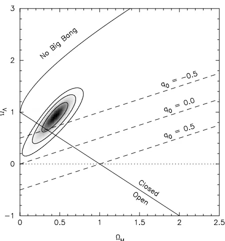
Figure 1.7: Constraints on ΩM and ΩΛ from SNe Ia observations. 1, 2 and 3-σ confidence

limits are indicated on theχ2 probability map. Data from Riess et al. (2004).

While it was known that the Universe contains a significant amount of ordinary matter that causes the expansion of the Universe to decelerate, the presence of other forms of energy, such as Einstein’s vacuum energy, the so-called ‘cosmological constant’, were unknown, until observations of distant type Ia supernovae (SNe Ia) showed that the expansion of the Universe was accelerating (Riess et al., 1998; Perlmutter et al., 1999), requiring a non-zero cosmological constant, or dark energy. By measuring the redshifts and apparent brightness of SNe Ia with known intrinsic brightness, the distances to these objects can be determined. It was found that the distances of the highest redshift SNe Ia are, on average, 10%₋15% further than expected in a low mass density universe without a cosmological constant. It is the energy density of matter, ΩM, and the energy density

of dark energy, ΩΛ, that determine the nature of the expansion of the Universe, and the

current best measurements from SNe Ia, assuming a flat Universe, is ΩM = 0.29+0−0..0503

(and ΩΛ = 0.71 correspondingly) (Riess et al., 2004). Current constraints on ΩM and ΩΛ

are shown in Fig. 1.7. However, very few SNe Ia have been observed at redshifts past z= 1, yet it is at redshifts greater than this that a ΩM = 0.3, ΩΛ = 0.7 universe varies

(38)

[image:38.595.168.506.66.269.2]

Figure 1.8: The magnitude difference between the distance modulus of 3 different cos-mologies and an empty cosmology (i.e., Ω = 0.0, dotted line) as a function of redshift,z. Solid line has ΩM = 0.3, ΩΛ = 0.7. Dashed line has ΩM = 0.0, ΩΛ= 1.0. Dashed-dotted

line has ΩM = 1.0, ΩΛ= 0.0.

Two of these direct methods include using the Sunyaev-Zeldovich effect (Sunyaev & Zeldovich, 1972; Silk & White, 1978; Sunyaev & Zeldovich, 1980) and using gravitational lens systems (Refsdal, 1964). The Sunyaev-Zeldovich (SZ) effect is the decrease in bright-ness temperature of the cosmic microwave background (CMB) due to the presence of hot gas in galaxy clusters. To determine a distance to the cluster, X-ray observations are used to determine the temperature and surface-brightness distribution of the cluster gas, where-as radio/sub-mm observations are used to determine the cooling of the CMB in the cluster direction. A combination of both observations, with some assumptions about the spatial distribution of the gas, leads to a measurement of the angular diameter distance to the cluster. This has been used to determine Hubble’s constant. Schmidt et al. (2004), for example, have foundH0 = 69±8 km s−1 Mpc−1 assuming ΩM = 0.d3 and ΩΛ= 0.7,

whereas Bonamente et al. (2005) combine observations of 38 galaxy clusters to determine 74 < H0 < 78 km s−1 Mpc−1, with the range of values due to different assumed gas

models. In the gravitational lens method, a measurement of the time delay between two gravitationally lensed images of an intrinsically variable quasar leads to a determination ofH0, provided there is a good model for the mass distribution of the lensing galaxy. The

(39)

references therein). Typical time delays are of the order of 30-100 days. A simple average ofH0values determined by this method givesH0 = 61±7 km s−1 Mpc−1(Courbin, 2003).

The use of AGN accretion discs as a way of determining H0 and putting constraints on

ΩM and ΩΛ provides another direct method that is independent on the distance ladder

(see Chapter 3 for further discussion).

1.5 X-ray Binaries

X-ray binaries (see Fig 1.1) are binary systems where the donor star accretes onto a compact object (either a neutron star or a black hole) and, when actively accreting, are the brightest persistent X-ray sources in the sky. They provide an ideal laboratory to study strong gravitational fields - the inner accretion flow onto stellar mass black holes and low-magnetic field neutron stars is only at a few Schwarzchild radii (RS = 2GM/c2) where

spacetime is strongly curved. They also allow an opportunity to constrain the equation of state of ultradense matter at the core of neutron stars, which leads to an understanding of the properties and behaviour of matter under extreme densities, through studying their fundamental properties such as the radius and mass.

(40)

star is a Be star, which possesses a circumstellar disc, and the compact object has a highly elliptical orbit, then as the compact object passes through the circumstellar disc it will accrete matter and emit X-rays. In HMXBs, the massive star dominates the emission of optical light, whereas accretion onto the compact object is the dominant source of X-rays. The O/B stars are luminous and therefore easily detected in the optical. The evolution of the high-mass companions in HMXBs determines their lifetime, which is short (105₋107 yr), and therefore they are distributed along the Galactic plane (as young stellar populations do). In contrast, the lifetime of LMXBs is much longer (107₋₁₀9 _yr)

and they tend to be concentrated towards the Galactic centre and in globular clusters. See fig. 1 of Grimm et al. (2002) for an illustration of the distribution of the LMXB and HMXB populations within the Galaxy. For a recent detailed review of accreting neutron stars and black holes the reader is referred to the book by Lewin & van der Klis (2006).

Further evidence for a difference in the age of the HMXB and LMXB populations comes from the presence of X-ray pulsations, or lack thereof. Interestingly, almost all HMXBs show X-ray pulsations indicating that compact object is a strongly magnetized neutron star with field strengths a few times 1012 _{G (e.g., Pringle & Rees, 1972; Bildsten}

et al., 1997). In these systems, material from the accretion disc is channelled onto the neutron star magnetic poles. If the magnetic and rotational axes are aligned differently, then pulsations in the X-ray lightcurve will be seen at the neutron star spin frequency as the magnetic poles rotate through the line of sight. LMXBs, on the other hand, rarely show X-ray pulsations, which is explained by the fact that the neutron stars in HMXBs are young, and therefore are strongly magnetized and rapidly rotating. In contrast, neutron stars in LMXBs are generally significantly older. Whilst they will have initially spun-down as energy is radiated at the expense of stored rotational energy, once accretion begins, they become spun up again. This leaves a weakly magnetized neutron star with B _∼ 108 G, although the process of the decrease in magnetic field is not understood (Bhattacharya & Srinivasan, 1995). However, the discovery of a millisecond X-ray pulsar in the LMXB SAX J1808.4₋3658 (Wijnands & van der Klis, 1998), showed that over time, accretion onto the neutron star in LMXBs can lead to it being spun-up to millisecond periods, leaving a weakly-magnetized, rapidly rotating neutron star, which once accretion halts becomes a millisecond radio pulsar.

(41)

by determining the mass of the compact object (neutron stars should not be heavier than around 3 M¯, see below) through optical radial-velocity data of the companion star. Even with only the mass function for the companion determined (through the orbital period and absorption-line velocity amplitude), this puts a lower limit on the mass of the compact object, and hence can determine whether or not it can be a neutron star. Black holes can be ruled out easily if a property that can be associated with a neutron star is seen, for instance, X-ray pulsations or type I X-ray bursts (thermonuclear flashes on the surface of a neutron star, Lewin, van Paradijs & Taam, 1995; Bildsten, 1998). Unfortunately, however, there are no such clean-cut distinctive characteristics that are only seen in black hole binaries.

1.5.1 Transient Low-mass X-ray Binaries

While many of the LMXBs are persistent sources and always actively accreting, there is a group of LMXBs that are transient. These transients spend the vast majority of their time in a quiescent state, during which very little or no accretion onto the compact object occurs. Occasionally, however, these systems go into outburst, which usually last weeks to months, throughout which they increase greatly (by a factor of around 104, though it can be as much as 109_{) in brightness. Such outbursts arise due to a significant increase in the}

(42)

During outburst the optical spectra of LMXBs show a few emission lines, especially Balmer lines, due to reprocessing of X-rays in the disc which dominates over the viscous heating within the disc. Usually, the companion star is not observable (unless the compan-ion star is evolved), and the optical spectrum is totally unlike an ordinary star. However, when in a quiescent state optical emission in the system is dominated by the companion star rather than by X-ray heating of the accretion disc, which is not important in this state (e.g., van Paradijs & McClintock, 1995; van Paradijs, 1998).

The work on X-ray binaries in this thesis focuses on the quiescent emission from neutron star X-ray binaries. We therefore review the emission processes involved, and compare with black hole quiescent emission. Before discussing quiescent emission from neutron star X-ray binaries, it is relevant to briefly outline the structure of a neutron star and their formation, as the various components play an important part in the quiescent emission.

1.5.2 Neutron stars

Neutron stars are very small (radius_∼10 - 20 km), dense, stars with masses between about 1.4 and 3.0 M¯, with the core composed of degenerate neutron gas, or more exotic forms of matter. They are one of the few possible endpoints of stellar evolution. Neutron stars cannot be more massive than around 3.0 M¯ (this limit is not known well due to the lack of knowledge of the equation of state for neutron-degenerate matter) as gravitational forces would overcome the degenerate neutron gas pressure, causing gravitational collapse, and the formation of a black hole (Srinivasan, 2002). Stars formed at the end of stellar evolution with a mass lower than about 1.4 M¯ are white dwarfs and are supported by degenerate electron gas pressure rather than a degenerate neutron gas. The neutron star radius depends on the mass, with more massive neutron stars having smaller radii. The high density of neutron stars leads to a high surface gravity and a substantial gravitational redshift for light emitted from the surface.

(43)

hundred metres down is the outer crust consisting of atomic nuclei and electrons. The electrons form a degenerate gas, whereas the nuclei are solid in most of the outer crust. At the base of the outer crust we get to the ‘neutron drip’ layer where it becomes energetically favourable for neutrons to drip out of the nuclei and move around freely forming a neutron gas between the nuclei. This ‘neutron drip’ layer marks the boundary between the inner and outer crust. The next 1 km or so down is theinner crustwhich consists of electrons, free neutrons and neutron-rich atomic nuclei (Haensel, 2003). As the depth (and therefore density) increases, the fraction of free neutrons also increases.

Below the inner crust is the stellar core where all the constituents are strongly degenerate and it is here where the neutron star structure is least certain. The outer core consists of mainly neutrons with several percent being protons, electrons and maybe muons. The size and content of the inner core, which could be as big as several kilometres, has a number of (exotic) possibilities. It could contain nucleon matter, basically the same as the outer core. Other possibilities include hyperonic matter, a pion condensate, a kaon condensate or even a quark fluid. The state of the matter in the core is important for neutron star cooling, as it determines the rate of neutrino emission - an important process in neutron star cooling. A good understanding of the cooling of neutron stars can therefore lead to a greater understanding of the deep interior of neutron stars (Yakovlev & Pethick, 2004).

The temperature at the surface of the neutron star is dependent on the temperature of the core and on the composition of the outer 100 m of the neutron star - the atmosphere and the outer crust (Brown, Bildsten & Chang, 2002). In accretion-heated neutron stars (the ones that are relevant to this thesis) the temperature of the core is around 108 K, and is constant for timescales of _≤104 _{yr (Brown, Bildsten & Rutledge, 1998), whereas}

(44)

Figure 1.9: A diagram outlining the structure of a neutron star (not to scale).

significantly as the density (and temperature) increases and the structure of the star changes from containing degenerate electrons in the outer crust to increasing amounts of free neutrons from the inner crust to the core (Gudmundsson et al., 1983). Whilst the core temperature is constant for timescales of _≤ 104 yr, the outer envelope can change temperature on timescales of days (Brown et al., 2002). Energy given to the outer envelope of the neutron star during accretion is generally radiated away due to the steep thermal gradient. However, when nuclear reactions are ignited in the inner crust due to compression by accreted material the core can be heated (Brown et al., 1998, see the section below on quiescent emission from neutron stars).

1.5.3 Neutron Star Formation in Low-Mass X-ray Binaries

(45)

The origin of a binary with a low mass companion and a neutron star is initially a little perplexing - one might quite reasonably expect that it would difficult to keep the companion bound to the binary in a supernovae explosion because more than half the mass of the binary will be lost in the explosion. Also, the current orbits of LMXBs are too small to have accommodated the progenitor to the neutron star. Three basic solutions to this problem are: (i) the supernova explosion was relatively quiet, resulting from accretion induced collapse of a white dwarf, (ii) the neutron star was born outside the binary and captured (this most likely applies to the formation of LMXBs in globular clusters), and (iii) the binary loses most of its initial mass and angular momentum during a ‘spiral-in’ phase. In the last case, as the neutron star progenitor (the more massive star in the binary) evolves it will expand and engulf the companion forming a common envelope. The friction from the common envelope causes the orbits to shrink, which in turn can cause the ejection of the common envelope. Thus, this common envelope phase will reduce both the mass of the progenitor and the size of the orbit. Finally, the remaining core continues to evolve and turn into a supernova. See Verbunt & van den Heuvel (1995) for a detailed review of the formation and evolution of neutron stars in X-ray binaries. We leave further discussion of the formation of LMXBs in globular clusters to the next section.

1.5.4 Low-Mass X-ray Binaries in Globular Clusters

(46)

[image:46.595.130.544.70.279.2]

Figure 1.10: Optical and X-ray images of the globular cluster 47 Tucanae. The Chandra X-ray image is false colour - with red indicating soft X-rays, and blue hard X-rays. The optical image of the globular cluster 47 Tuc was taken with the Euro-pean Southern Observatory’s Danish 1.54-m Telescope at La Silla, Chile. Credit: X-ray: NASA/CXC/CfA/J.Grindlay & C.Heinke; Optical: ESO/Danish 1.54-m/W.Keel et al.

this phase. The known distance and reddening allows accurate luminosities to be derived and removes the distance uncertainty from the properties. All the low-luminosity X-ray sources in globular clusters (at least to current detection levels) are binary systems (active binaries, CVs, LMXBs). Thus, studying globular clusters in X-rays allows us to study the binary content of globular clusters and how that might evolve in time.

(47)

Figure 1.11: Number of globular cluster X-ray sources (N) with LX ≥4×1030 ergs s−1

vs. the normalised encounter rate, Γ of the cluster. An arrow indicates a globular cluster for which theChandra observation did not reach the required sensitivity. The dashed line indicates the best-fitN _∝Γ0.74. From Pooley et al. (2003), courtesy of Dave Pooley.

a neutron star with a red giant, followed by orbital decay (Sutantyo, 1975; Ivanova et al., 2005). As the neutron star enters the giant’s atmosphere, it is slowed down. If it leaves the giant’s atmosphere with a velocity less than the escape velocity, (2GMtot/R)1/2, then

it will be captured in a close binary orbit. The passage of the neutron star through the red giant’s atmosphere will cause the common envelope to be disrupted, hence, these collisions produce tight, eccentric neutron star-white dwarf binaries (Rasio & Shapiro, 1991).

(48)

1.6 Quiescent Emission from Neutron Stars

Well over a dozen neutron star X-ray transient systems have been detected in quiescence as well as in outburst. The quiescent luminosity of these neutron star systems is typically 1032₋1034 erg s−1 (though some are fainter) compared to typical outburst luminosities in the range 1036₋1038 erg s−1. One way to investigate the source of this emission, is to study the X-ray spectra. The X-ray spectra of these quiescent neutron star systems are generally characterised by two components: a soft component (which dominates the spectra below a few keV), equivalent to a blackbody temperature of kT _∼0.1₋0.3 keV, and a hard power-law tail (which dominates the spectra above a few keV).

The mechanism most often used to explain the thermal X-ray emission from neutron star transients in quiescence is that in which the emission is due to the cooling of a hot neutron star which has been heated during outburst (van Paradijs et al., 1987; Brown et al., 1998). In the Brown, Bildsten & Rutledge (1998) model, during each outburst the neutron star core is heated by nuclear reactions occurring deep in the crust that are induced by compression of matter during accretion. After a period of around 104 years, the core is heated to a steady state, and is maintained at temperatures around 108 _{K by}

recurrent outbursts. This hot neutron star then emits thermally during quiescence. The temperature of the neutron star core and surface in quiescence is set by the time-averaged (over the neutron star thermal timescale) mass accretion rate, such that the quiescent luminosity is given by (Brown et al., 1998; Rutledge et al., 2002b)

Lq= 8.7×1033

Ã

hM˙_i 10−10_M

¯ yr−1 !

Q

1.45 MeV ergs s

−1 _, _(1.12)

where _hM˙_i is the time-averaged mass accretion rate onto the neutron star and Q is the amount of heat deposited in the crust per accreted nucleon and when assuming standard neutron star core cooling model. For an accretion flux onto the neutron star, Facc =

²M c˙ 2_/(4πD2_{), the ‘rock bottom’ quiescent flux due to deep crustal heating is then}

Fq≈ h

Facci

135

Q 1.45 MeV

0.2

² (1.13)

where _hFacci is the time-averaged accretion flux, and the accretion efficiency ² = 0.2 for

an accretion luminosity ofGM_hM˙_i/R.

(49)

f = (R/D)2σT4, where the flux,f, and the temperature T, can be measured from X-ray spectral fitting. One criticism of the thermal emission hypothesis had been that blackbody spectral fits to quiescent spectra vastly underestimated the emitting area, withR_≈1 km (Rutledge et al., 2000, and references therein). However, when realistic neutron star at-mosphere model spectra are used (for example the model by Zavlin, Pavlov & Shibanov, 1996) realistic emitting areas of around 10 km are found (e.g., Rutledge et al., 1999, 2000). The neutron star atmosphere models used are for a pure hydrogen atmosphere and for a weakly magnetized neutron star (with B < 1010 _{G, as expected for neutron stars in}

LMXBs). The atmosphere is expected to be nearly pure hydrogen as the accreting metals will gravitationally settle faster than they are supplied. The reason for the difference in measured emitting area between blackbody and neutron star atmosphere models is due to a slight difference in shape of the spectra. The opacity in the hydrogen atmosphere is dominated by free-free absorption, which is highly frequency dependent (_∝ν−3). There-fore, higher energy (frequency) photons escape from deeper (and thus hotter) regions in the atmosphere than the less energetic photons (Pavlov & Shibanov, 1978; Rajagopal & Romani, 1996; Zavlin et al., 1996). This makes the spectrum harder than a blackbody, and so any attempted blackbody fit will result in a systematically higher temperature and lower emission radii.

When published, the Brown et al. (1998) model was able to explain the luminosities of the majority of quiescent neutron-star transients, however, there are some exceptions, such as Cen X₋4 (Rutledge et al., 2001b) that are cooler than expected given their known accretion histories. This is generally explained by assuming that enhanced core cooling processes (as opposed to the standard processes assumed by Brown et al., 1998) occur. We leave further discussion of this to Chapters 4, 5 and 6 where we investigate and discuss quiescent neutron-star transient luminosities further. However, at this point, it is worth briefly mentioning the difference between ‘standard’ and ‘enhanced’ core cooling processes. The difference is due to the level of neutrino emission from the core. Neutrinos carry away energy, and provide an efficient way of cooling warm neutron stars. The dominant neutrino cooling reactions are known as Urca processes2 (see, e.g., Yakovlev & Pethick, 2004; Lat-timer & Prakash, 2004). In this process thermally excited particles alternatively undergo 2_{‘Urca’ is, quite surprisingly, not another astronomical acronym, but the name of a casino in Rio de}

Janeiro at which George Gamow commented to Mario Schoenberg “the energy disappears in the nucleus

of the supernova as quickly as the money disappeared at that roulette table.” (Gamow & Schoenberg,

(50)

beta and inverse-beta decays, with each reaction producing a neutrino or antineutrino. The most efficient Urca process is the direct Urca process involving nucleons:

n_→p+e−+ ¯νe, p→n+e++νe. (1.14)

This can only occur if both energy and momentum are conserved simultaneously. If this is not possible, then the modified Urca process can take place, in which a bystander baryon absorbs momentum:

n+ (n, p)_→p+ (n, p) +e−+ ¯νe, p+ (n, p)→n+ (n, p) +e++νe. (1.15)

In standard cooling models, the modified Urca process is the neutrino emission that takes place. However, in enhanced cooling models, where the level of neutrino emissions is higher, the direct Urca process is usually invoked. Enhanced cooling via the direct Urca process requires that the neutron star is more massive than the canonical value of 1.4 M¯, with a mass around 1.7 M¯ (Colpi et al., 2001). There are, however, other processes that increase neutrino emissions such as the breaking of nucleonic Cooper pairs (e.g., Flowers et al., 1976; Gusakov et al., 2004), or processes similar to the direct Urca process, but involving pion or kaon condensates, or quark matter (Yakovlev & Pethick, 2004).

Nevertheless, back to the discussion on the thermal emission from neutron stars. Whilst the cooling of an accretion-heated neutron star is the most widely accepted model for the thermal emission, there are alternative models that have been proposed (see Cam-pana et al., 1998a, for a detailed review of the possibilities). For instance, continued accretion onto the neutron star surface at a low level during quiescence can produce a thermal-like spectrum (Zampieri et al., 1995). Another possibility is low-level accretion down to the magnetospheric radius (Menou et al., 1999; Menou & McClintock, 2001) where accretion onto the surface is prevented due to the propeller effect - when the magneto-sphere is beyond the co-rotation radius, centrifugal force prevents material from entering the magnetosphere, and thus accretion onto magnetic poles ceases (Pringle & Rees, 1972; Lamb et al., 1973).

(51)

et al. (2004b) found that the power-law contribution is low only when the source quiescent luminosity is close to _∼ 1₋2_×1033 _{erg s}−1_{, and that both at lower values the}

power-law contribution to the 0.5-10 keV luminosity increases. Possible mechanisms for the emission of this power-law component include residual accretion onto the neutron star magnetosphere (as mentioned above) or a putative pulsar wind colliding with infalling matter from the companion star (Tavani, 1991; Campana et al., 1998a). Whilst the ‘rock-bottom’ flux may be set by the cooling neutron star, additional residual accretion may cause the power-law component. This can explain some variability seen in quiescence (this will be discussed in detail in Chp. 4).

Finally, some X-ray transients (the quasi-persistent transients) spend an unusually long time in outburst, with outbursts lasting years to decades rather than the more com-mon weeks to com-months. During outbursts, the crust of the neutron star is heated to a point beyond thermal equilibrium with the stellar interior. Once accretion falls to quiescent lev-els, the crust cools thermally, emitting X-rays, until it reaches equilibrium again with the core (e.g., Wijnands et al., 2002a; Rutledge et al., 2002b). Whilst in ‘normal’ transients the crust and core reach thermal equilibrium in days, it can take months to years for the quasi-persistent sources. These sources allow us to probe the cooling mechanisms at work in neutron stars, and set limits on the structure of the core. These sources are the focus of Chp. 6.

1.6.1 Quiescent Emission from Black Holes