Model Predictive Direct Flux Vector Control of
Multi Three-Phase Induction Motor Drives
S. Rubino
1,
Student Member, IEEE
, R. Bojoi
1,
Senior Member, IEEE
,
S.A. Odhano
2,
Member, IEEE
, P. Zanchetta
2,
Senior Member, IEEE
1Politecnico di Torino, Dipartimento Energia, Torino, 10129, Italy
2Department of Electrical and Electronic Engineering, University of Nottingham, Nottingham, NG7 2RD, United Kingdom
Abstract—A model predictive control scheme for multiphase induction machines, configured as multi three-phase structures, is proposed in this paper. The predictive algorithm uses a Direct Flux Vector Control scheme based on a multi three-phase approach, where each three-phase winding set is independently controlled. In this way, the fault tolerant behavior of the drive system is improved. The proposed solution has been tested with a multi-modular power converter feeding a six-phase asymmetrical induction machine (10kW, 6000 rpm). Complete details about the predictive control scheme and adopted flux observer are included. The experimental validation in both generation and motoring mode is reported, including open-winding post-fault operations. The experimental results demonstrate full drive controllability, including deep flux-weakening operation.
Keywords—multiphase induction machines; multiphase drives; model predictive control; fault-tolerance; direct flux vector control.
I. INTRODUCTION
In the recent years, the model predictive control (MPC) of electrical drives has gained an impressive attention. In this context, a relevant development has been reached in the predictive torque control [1-6] that presents several advantages. Its most salient feature is the improvement of the dynamic torque response, generally better than traditional feedback controls [3]. Another aspect is a less demanding calibration of the control parameters and settings [6]. On the other hand, the use of predictive algorithms requires a good estimation of the machine’s parameters and, in general, a greater computational power with respect to traditional control strategies. In this field of research, an advanced development has been reached in the Finite Control Set Model Predictive Control (FCS-MPC) for three-phase machines [2,4-6]. With FCS-MPC, the voltage references are chosen from the instantaneous discrete states of the power converter to minimize a user-defined cost function.
Important limitations on the use of FCS-MPC schemes consist in the current’s derivatives that can reach uncontrollable values, especially with low impedance machines (for example in traction motors). In fact, the behavior of the FCS-MPC is very similar to the well-known Direct Torque Control (DTC) implemented at low switching frequencies.
The multiphase drive systems are considered today as a viable solution for high power/high current applications and for applications that require redundancies to achieve fault tolerance, such as electric ship propulsion and generation, railway traction, more-electric-aircraft, high speed elevators, wind energy generation and hybrid/electrical vehicles [7-15]. The main benefits of multiphase drives include the reduction of the phase
current without increasing the phase voltage and the fault-tolerant nature. The increase of the phase number will increase the system complexity, so the application of the FCS-MPC methods on multiphase machines will require a very high computational power of the dedicated control hardware. In the multiphase systems, the number of power converter’s discrete states becomes very high [16-19], therefore the minimization of a cost function for every sample time (which in many cases is the same as the switching period or a half of it) is less viable.
A possible solution to solve these issues can be the adoption of a Continuous Control Set Model Predictive Control (CCS-MPC). The main difference with respect to the classical finite-set types is the selection of the voltage references. In fact, it is performed in the range of all possible average voltage vectors, which the power converter can apply. This control strategy is usually known as Modulated Model Predictive Control (M2PC)
using Pulse-Width or Space Vector Modulation [6] (PWM or SVM). Another predictive solution based on average voltage vectors applied at constant switching frequency is the Dead-Beat Direct Torque and Flux Control (DBTFC). As example, the solution presented in [20] for three-phase induction machines contains a dead-beat control law based on a Volt–second-based torque model to produce the desired torque and stator flux magnitude simultaneously.
The literature reports a few predictive control solutions applied to multiphase induction motor drives [18, 19] without flux-weakening operation. The solution presented in [18] is related only to the current control using FCS-MPC of an asymmetrical six-phase induction machine prototype exhibiting high inductance values. There is no evidence that an attempt has ever been made to propose a complete MPC control solution for a multiphase motor drive able to deal with flux-weakening operation and with sudden open-phase faults.
The goal of the work is therefore to propose a dead-beat model predictive control for multiphase Induction Motor (IM) drives configured as multi three-phase units. The contributions of the paper are the following:
The dead-beat predictive algorithm is implemented on the basic structure of the Direct Flux Vector Control (DFVC) scheme for simultaneous flux and torque control with no need of tuning after the implementation.
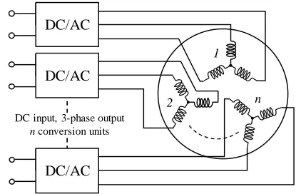
Fig. 1. Multiphase topology with multiple three-phase units.
Maximum Torque per Volt (MTPV) operation with load angle limitation at flux-weakening.
Open-winding fault ride-through capability for sudden turn-off of one three-phase set.
The performance of the proposed control has been validated with a 10kW, 6000 rpm asymmetrical six-phase induction machine that uses a double three-phase stator winding configuration. This paper extends the results that have been presented in [21] with the performance at deep flux-weakening, including the MTPV operation with load angle limitation.
The paper is organized as follows. The description of the drive topology and of the machine modeling are analyzed in Section II. The formulation of the model predictive algorithm is described in Section III. The proposed predictive control scheme is described in Section IV, while the test rig and the experimental results are provided in Section V. Finally, Section VI concludes the paper.
II. MULTIPHASETOPOLOGY ANDMACHINEMODELING
A. Multi Three-Phase Topology
The multi three-phase topology uses multiple independent three-phase units (Fig. 1). The stator consists of three-phase winding sets with isolated neutral points. An independent three-phase inverter supplies each three-three-phase set. The inverter units share the control algorithm only at high level to obtain full fault-tolerance. If a three-phase inverter unit develops a fault, it is disconnected from the DC power supply. The main advantage of this configuration is the use of the well-consolidated three-phase power electronics modules, reducing the converter size, cost and design time [11].
B. Machine Modeling
The mathematical description of the multi three-phase topology can be performed by using the Multi-Stator (MS) approach. Introduced in [22] and recently applied in [23] for a quadruple three-phase machine, MS considers the stator as a multiple of phase sets, while the rotor is seen as a three-phase structure [24].
This section presents a generic MS modeling approach for an Induction Machine (IM) with the hypothesis of sinusoidal winding distribution. The number of phases of the machine is nph=3n and k=1,2,…,n is the index number of a single three-phase set. The stator parameters of the three-three-phase sets are considered different from one another in order to deal with the most generic case. For simplicity, the iron losses are neglected.
For each three-phase statork-set, the stator voltage equations are:
sabck
sk
sabck
sabck
dt d i
R
v , , , (1)
where:
xsabc,k
xsak xsbk xsck
tis a stator vector definedfor the three-phase set (abc)kand defined in own stator coordinates;
sk
R is the stator resistance ofk-set.
Assuming a rotor cage that is equivalent to a three-phase wound rotor, the rotor voltage equations are:
rabc
r
rabc
rabc
dt d i R
v [0] (2)
where:
xrabc
xra xrb xrc
tis a rotor vector in rotor phase coordinates;r
R is the rotor resistance.
The IM magnetic model is described by (3) and (4):
sk r
rabc
n
z
z sabc sz sk k
sabc lsk k
sabc L i M i M i
1
, ,
, (3)
r r
rabcn
z
z sabc sz r rabc
lr
rabc L i M i M i
1
, (4)
where:
Msksz
is a 33 mutual inductance matrix between thestator windings ofk-set and the stator windings ofz-set;
Mskr
is a 33 mutual inductance matrix between the stator windings ofk-set and the rotor;
Mrsz
is a 33 mutual inductance matrix between the rotor and the stator windings ofz-set;
Mrr
is a 33 mutual rotor inductance matrix; lskL is the stator leakage inductance ofk-set;
lr
L is the rotor leakage inductance.
All rotor parameters from (2-4) are referred to the stator. The MS approach needs the application of the general Clarke transformation to get the machine model in stationary (,β) frame:
2 1 2
1 2
1
3 2 sin 3 2 sin sin
3 2 cos 3 2 cos cos
3 2
k k
k
k k
k
k
T (5)
wherekis the angle considered for the three-phasek-set; this angle is defined as the position of the first phase (a-phase) of the k-set with respect to the -axis. By applying (5) to (1-4), the stator model for the IM in (,β) reference frame becomes:
, ,
, sk sk sk
sk
dt d i
R
v (6)
The rotor equations are transformed into stator stationary reference frame using (5) with k = r, where ris the rotor electrical position:
, , ,
0 r r r j r r
dt d i
R (7)
where ωr=p ωmis the rotor electrical speed,pis the pole-pairs
number, ωm is the mechanical speed computed from the
mechanical rotor positionm.
DC input, 3-phase output
nconversion units
1
2 n
DC/AC
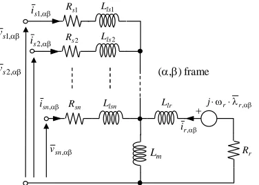
Fig. 2. Equivalent circuit of a multi three-phase IM in stationary (α,β) frame.
The IM magnetic model (current-to-flux relationship) in the stationary frame is:
, 1 , ,, m r
n z sz m sk lsk
sk L i L i L i (8)
, 1 , ,, m r
n z sz m r lr
r L i L i L i (9)
where Lm is the magnetizing inductance.
The IM electromagnetic torque is given by (10) and represents the sum ofnouter (vector) products:
n z sz sz i p T 1 , , 2 3 (10)According to (6-10), the MS approach definesn different stator flux linkage vectors and current vectors and the total electromagnetic torque is the sum of the contributions of then stator sets that interact with the three-phase rotor. Therefore, the equivalent circuit of the IM corresponding to the MS modeling approach is shown in Fig. 2.
The stator and rotor equations can be referred to a generic rotating reference frame (d,q) at the speed e. Indeed, by applying the conventional rotational transformation, the (d,q) voltage equations become:
dq sk e dq sk dq sk sk dq sk j dt d i R
v , , , , (11)
e r
rdqdq r dq r r j dt d i
R , , ,
0 (12)
The IM magnetic model in rotating (d,q) frame is formally identical with (8-9), with the difference that all vectors (fluxes and currents) are referred to the (d,q) frame instead of the (,β) stationary reference frame.
III. MODELPREDICTIVEFORMULATION
The implementation of a predictive system requires first the computation of the machine’s state equations and a good method to discretize them. This procedure is well consolidated for three-phase machines but not for multi three-three-phase configurations having a higher number of active state variables.
A. Machines’s State Equations
The proposed model predictive algorithm uses a DFVC scheme based on the MS-approach [21-26]. Consequently, the stator currents and the stator fluxes must be considered as main state variables. It is necessary to introduce the following preliminary variables: lr m m r L L L k , lsk m m sk L L L k , r lr m r R L L (13)
n k z z lsz z lr r k L x L k c 1 , lsz z lr r z L x L kc (14)
where ݔ௭ is a logic value depending on the state of the consideredz-set (0 off, 1 on). In this way, it is possible to adapt the equations of the remaining active sets after open-windings fault events.
The state equations with the MS approach for a singlek-set (k=1,2,…,n) leads to:
k dq sk k v dq sk eq dq sk k eq dq sk k
eq Z i f k v C
dt i d
L , , , , , , , (15)
dq sk e dq sk dq sk sk dq
sk R i v j
dt d , , , , (16)
n z dq sz r r dq r slip r dqr j R k i
dt d 1 , , 1
, ( ) (17)
where: Leq,k(1ck)Llsk krLlr )
( , ,
,k eqk eqk
eq R j X
Z
k
sk sk
r r k
eq R c
k k R
R , 1
k eq slip lsk k r k
eq c L L
X , ,
r r
eq j
f 1 , kv,k 1ck,slip er The term Ck contains the coupling terms between the consideredk-set with the other onesz=1,2,…,n,z≠k. This is the direct consequence of the application of MS-approach with respect to the conventional Vector Space Decomposition (VSD) [17, 22]. The coupling termCkis computed as:
n k z z dq sz z eq dq sz zk c v Z i
C 1 , , , ) ( (18)
where: Zeq,z Req,z jXeq,z
z sz r r z
eq R k R c
R , , Xeq,z rczLlsz
The equations (15-17) describe the complete
electromagnetic dynamic model of a multi-three phase machine with a generic number of three-phase setsnand represents the starting point for the implementation of any MPC solution. B. Discretization of the State Equations
The state equations (15-17) must be converted into their discrete time equivalents. This operation is not easy to perform, even for a three-phase case. In fact, it is necessary to compute the general relationships of the eigenvalues and related eigenvectors of a high order system. For this reason, in this work the Euler’s approximation is proposed.
Independent of the considered equation from the set (15-17), each of them has the same structure where from a side there is the derivative of the considered variableܺതwhile, on the other side, the forcing termsܨത:
) ( ) ,
(F t F t
X dt
d
(19)
sn
R Llsn Llr
m
L Rr
r r,
j , 1 s v , sn v , sn i
(,) frame , 2 s i , 1 s i , 2 s v 1 s R 2 s
R Lls2
Fig. 3. Multiple stator flux frames in the DFVC based MS-approach. The Euler’s approximation of (19) in order to convert the time domain from continuous to discrete is:
) ( ) ( ) 1 ( ) ( ) ( ) 1 ( F T X X F T X X S S (20)
where TS is the sample time for the discretization and τ the generic sample time instant. As an example, the application of (20) to (16) leads to:
) ( , , , , , 1 ,
skdq skdq TS Rsk iskdq vskdq j e skdq (21) The choice of Euler’s discretization is advantageous for a multiphase machine since it obtains simple first-order approximations of the real discrete equations involving multiple variables and coupling terms. The sampling timeTSdepends on the inverter switching frequency and therefore it is often predefined. Consequently, the accuracy of the Euler’s discretization will depend on the electric fundamental frequency along with a proper estimation of the machine’s parameters.
IV. MACHINECONTROLSCHEME
The application of a model predictive algorithm does not depend on the choice of the control type. In fact, MPC allows at improving the performance of already defined control scheme by replacing the traditional PI-controller with a better selection of the voltage references.
The proposed model predictive algorithm uses a DFVC scheme based on the MS-approach. The DFVC combines the advantages of a direct flux regulation (as for constant frequency direct torque control) with current regulation (as for vector control) [23, 25, 26]. The flux-weakening is straightforward without any need of additional voltage control loops [25], while the current limitation is simple to implement, as shown later.
The main advantage of the MS-approach is the possibility to build a modular machine control where each three-phase set is independently controlled. In this way, post open-winding fault or torque sharing operations become easy to perform. According to the torque demand and the operating speed, the MS-based DFVC aims at controllingnstator flux vectors innoverlapped stator flux frames (dsk,qsk,k=1,2,…,n), as shown in Fig. 3. A. Stator Flux and Torque Equations
The machine model in multiple stator flux reference frames (dsk,qsk,k=1,2,…,n) is described by the equations (15-17), where the synchronous speedecorresponds with the angular speed of the considered stator flux vector. In theory, this value must be defined set by set. However, since the machine control aims at settingnoverlapped stator flux frames, the differences between the three-phase sets can be neglected.
[image:4.595.83.239.60.181.2]Fig. 4. Predictive DFVC scheme of a generic multi three-phase IM machine.
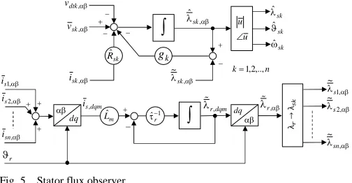
Fig. 5. Stator flux observer.
Relevant attention must be given to the stator flux (16) and torque (10) equations. In fact, the DFVC is implemented in rotating stator flux frame and this leads to important simplifications. In terms of stator flux vectors, each of them is aligned in the own dsk-axis and so all qsk-axis stator flux components are zero:
ds sk ds sk sk
sk R i v
dt d , , (22)
The total electromagnetic torque is:
n k qs sk sk i p T 1 , ) ( 2 3 (23)The model (22)-(23) leads to the following considerations:
Thedsk– axis voltage (vsk,ds) directly imposes the stator
flux magnitude λsk,k=1,2,...,n.
The torque contribution of one stator winding k-set is controlled by regulating the corresponding qsk – axis current (isk,qs), using the voltage component vsk,qs, k=1,2,...,n.
The proposed predictive DFVC scheme is shown in Fig. 4 and the description of the different blocks is reported below.
B. Stator Flux Observer
The flux observer is shown in Fig. 5. It estimatesnstator flux
vectors , ˆ
sk ,k=1,2,…,n, corresponding to thenstator
three-phase sets. The flux observer is based on the back-EMF integration at high speed and on the rotor magnetic model at low speed [27].
-axis
-axis
qsk-axis
k =1,2,...,n
dsk-axis
sk
i sk
r sk n sabc
i ,1
DT LUT , 1n s i , 1n dt v Direct Clarke Stator flux observer Speed computation m
m
Voltage Reconstruction PWM * 1 , n abc dc v , 1n s v * , 1n
s v * 1 , n sabc v Inverse Clarke Model Predictive
Estimator 1,
ˆ n s Model Predictive DFVC * T max I 1 1
ˆ s n
1 1 ,
ˆ
s n
i ˆ11
s n
n s ˆ1
3 3
3
IM 3n-ph
dc
v
n s ˆ1
, 1n s v , 1n s i , 1n dt v
k g , sk v , dtk v , ˆ sk , ~ sk u u sk ˆ sk ˆ sk ˆ , ski k1,2,..,n
sk
Rˆ
dq dq , 1 s i , 2 s i , sn i
is,dqm
m
Lˆ
1, ~
s 2, ~ s , ~ sn 1 r ˆ r , r dqm
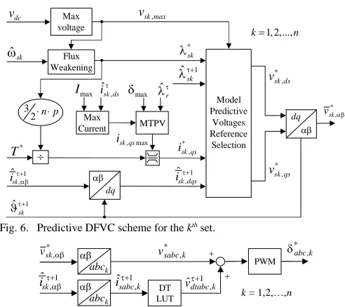
[image:4.595.307.559.237.368.2]Fig. 6. Predictive DFVC scheme for thekthset.
Fig. 7. Predictive compensation of Dead Time (DT) errors for thekthset.
At low speed, the stator flux vectors are computed from the rotor flux using (7-9). The rotor model is sensitive to the error in rotor time constantr, but this affects only the machine starting. At high speed, thek-set stator flux estimates depend only on the stator resistancesRsk. The detuning on this parameter has very low effects on the flux estimation, so the flux observer is very robust against parameters detuning. For each setk, the transition electrical frequency (rad/s) between the rotor model and the stator model [27] is equal to the observer gaingk.
To improve the performance at low speed, a dead-time (DT) compensation scheme has been implemented for each stator set using the solution described in [28].
C. Predictive Direct Flux Vector Control (DFVC) scheme
The proposed predictive DFVC scheme contains n
independent modules that are separately implemented in the overlapped stator flux frames (dsk,qsk,k=1,2,…,n), as shown in Figs. 6-8. A single DFVC module is operated as for a three-phase machine and does not interact with the other modules.
The reference flux is generated by a Flux-Weakening (FW) block that imposes the rated flux (corresponding to one statork -set) below the base speed and a flux that depends on the available DC link inverter voltage and the synchronous speed
sk
ˆ at flux-weakening. The torque-producing component in stator flux frame is computed for each statork-set as:
*
* *
,qs 1.5 sk
sk T n p
i ,k=1,2,…,n (24)
Apparently, the computation of theqs-axis reference current component using (24) may be a problem when the stator flux reference is zero. In practice, this situation never happens. At start-up, theqs-axis current regulation is engaged only after an
[image:5.595.335.524.60.169.2]initial fluxing period that is used to build the machine flux. Moreover, the reference fluxλ௦∗ from (24) is anyway limited at a non-zero low value that is lower than the minimum flux value required at flux-weakening operation with the maximum motor speed. The torque producing current references݅௦∗,௦for then stator sets are further limited according to the machine/converter maximum currentImax, as implemented in [25].
Fig. 8. Predictive voltages reference computation scheme for thekthset.
Furthermore, the torque producing current components must be limited to avoid violating the Max Torque Per Voltage (MTPV) limit of the machine, as implemented in [29, 30]. This limitation is mandatory when the torque reference is provided by an outer control loop to avoid possible instabilities. The limitations on the torque producing current components are performed sequentially (i.e. current limitation followed by the load angle limitationmax), as shown in Fig 6.
The flux computation at flux weakening is implemented as in [25]. The independent flux-current control of the stator sets keeps balanced their currents and allows the operation with one or more stator sets turned off in case of faults.
With respect to a conventional DFVC based on the MS approach [23,26], the application of a predictive algorithm requires additional blocks, as shown in Fig. 4. The first one is the Model Predictive Estimator (MPE) that performs the prediction of the variables of interest for the next sample time
instant (τ+1).
The MPE block implements the state equations (15-17) with the application of the Euler’s discretization (20). The prediction
of the variables is performed in the stationary frame (α,β) in
order to use the estimates of the stator flux observer directly. Therefore, the equations (15-17) are implemented by setting the synchronous speedeto zero.
The MPE presents a modular structure to preserve the control scheme modularity. In fact, it is structured innpredictive estimators where each of them performs the predictive estimation for the dedicatedk-set. The MPE provides the values of stator fluxes and stator currents for the next sample time
instant (τ+1). From the predicted values of the stator currents, it
is possible to estimate the Dead Time (DT) errors of the power
converter for the next sample time instant (τ+1). In this way, an
accurate feed-forward compensation of the inverter dead-time can be obtained, as shown in Fig. 7. This action leads to significant improvements in the current waveforms, especially at low speed and for no-load condition.
For eachk-set, the position of the stator flux vector ˆsk1for
the next sample time instant (τ+1) is computed to perform the
rotational transformations of the input/output variables.
The rotational transformation of the currents allows at
obtaining the (dsk,qsk) current values 1 ,
ˆ
sk dqs
i for the next sample
time instant (τ+1). However, the prediction of the angle ˆ1
sk is
also necessary to perform the rotational transformation for the
computation of the next sample time (τ+1) output reference
voltages vsk*,, as shown in Fig. 6.
Max voltage Flux Weakening * sk 1 ˆ sk , sk max v dc v ˆsk *
T sk qs, max
i * , sk ds v * , sk qs i p n 2 3 dq 1 ˆ sk 1 , ˆ sk
i ,1
ˆ sk dqs i dq * , sk v * , sk qs v Model Predictive Voltages Reference Selection , ˆ sk ds i max
I max
Max Current ˆ r MTPV 1, 2,...,
k n
k abc DT LUT 1 ,
ˆ k dtabc v * ,k sabc v PWM * ,k abc k abc * , sk v
k= 1,2,…,n
1 , ˆ sabc k i 1 , ˆ sk
i
*
sk
1
ˆ sk Inverse Flux Model max sk v , 1 u 2 u Inverse q-Current Model * ,qs sk i q-axis Voltage Decoupling
zk
1, 2,...,
z n
* , sk qs v * , sk ds v 1 , ˆ sk qs i * , k qs F * , z qs F 1, 2,...,
The predicted values of currents iˆsk dqs,1 and stator flux amplitudes ˆsk1, together with the references of stator flux
amplitude *sk and qsk-axis current isk*,qs, are used for the computation of the voltage references vsk*,, as shown in the Figs. 6-8.
D. Predictive Reference Voltages Selection
The proposed model predictive algorithm uses the machine inverse model for the control of the reference variables. Practically, the voltage references applied at the next sample
time instant (τ+1) establish the evolution of the state variables at the next step (τ+2):
) 1 ( )
1 ( ) 2
( X T F
X S (25)
From (25), to set the value of the generic state variableܺതto a target valueܺത∗it is necessary to satisfy (26):
S
T X X
F ( 1) ( 1)
*
* (26)
Referring to the equations (15-17), the application of (26) corresponds to invert the machine model in order to obtain the voltage references. The proposed method for the computation of the voltage references is shown in Fig. 8.
1) Voltage reference computation on dsk-axis
By considering (22), the computation of thedsk– axis voltage reference is performed as:
* 1
* 1
, ,
ˆ
ˆ ˆ sk sk
sk ds sk sk ds S
v R i
T
(27)
The dsk – axis voltage reference, together with the inverter voltage limit, defines the limits of theqsk– axis component, as in a conventional DFVC scheme.
2) Voltage reference computation on qsk-axis
With respect to thedsk– axis component, the computation of theqsk– axis reference voltage must be performed in two steps. In fact, theqsk– axis current equation (15) contains the voltage coupling between the sets.
Therefore, it is necessary to compute first the linear combinations of voltages reference as function of theqsk– axis current reference:
n
k z z
qs k qs sz z qs
sk k
v v c v F
k
, 1
* , *
, *
,
, ˆ
ˆ (28)
where:
,
* * 1 1 1 1
, , , , , , ,
1 1 1 1 1
, , , , ,
1,
ˆ
ˆ ˆ
ˆ ˆ ˆ
( ) ..
ˆ ˆ ˆ ˆ ˆ
ˆ
.. ( )
eq k
k qs sk qs sk qs eq k sk qs eq k sk ds S
n
r sk eq z sz qs eq z sz ds k comp
z z k
L
F i i R i X i
T
R i X i K
(29)
The eq. (29) contains a new term calledKk,comp that represents the output of an integral regulator and it is computed as:
1 *
, , , ( , ˆ , )
k comp k comp S i k sk qs sk qs
[image:6.595.306.540.54.298.2]K K T k i i (30)
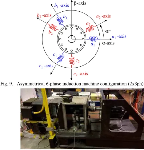
[image:6.595.39.287.552.658.2]Fig. 9. Asymmetrical 6-phase induction machine configuration (2x3ph).
Fig. 10. Machine under test (right) and the driving machine (left).
Apparently, the (30) represents the integral regulation of the qsk– axis current in a traditional DFVC scheme. Nevertheless, the purpose of this compensation is completely different. In fact, the predictive computation of the variables loses its accuracy at high frequency/speed, caused by the approximation of the Euler’s discretization. Furthermore, the predictive algorithm is based on the machine’s parameters and consequently is influenced by the estimation errors.
These problems cause torque permanent error, especially for the inaccuracy in theqsk– axis. Through the application of the integral regulation (30), the torque error converges to zero with the dynamics related to the value of the integral gainki,kand the voltage margin of the integral compensator (a good compromise is 5%-10% of the total phase voltage margin). The design of this regulator is not critical. It does not influence the dynamic behavior of the drive but only the steady-state operation.
From (28) it is necessary to extrapolate theqsk– axis voltage referencev*sk,qs. Therefore, it is necessary to apply the following decoupling operations:
1* * *
, , ,
1 1
ˆ 1 ˆ
n n
sk qs k qs z z qs z
z z
v F c F c
(31)The application of (31) is not critical and it is valid in case of open-winding fault events since cˆz are defined as (14).
V. EXPERIMENTALRESULTS
The performance of the proposed control has been validated with an asymmetrical six-phase induction machine. The main features of the machine are provided in Appendix. The stator has 6 phases with two slot/pole/phase, forming a double-three-phase winding with a relative shift of 30 electrical degrees among the two three-phase sets (akbkck), k=1,2, as shown in Fig. 9. The machine has been mounted on a test rig for development purposes. The shaft of the machine prototype is connected with a driving machine (Fig. 10) which acts as prime mover.
a1
a2
b1
c1
b2
c2
a2-axis
c1-axis
c2-axis
b2-axis
b1-axis
-axis
-axis
30
Fig. 11. Fast torque transient from 150% rated torque in motoring to 150% rated torque in generation at -6000 rpm, Set 1. From top to bottom: reference, observed and predicted torque (Nm); reference, observed and predicted stator flux (Vs); measured and predictedds-axis current (A); reference, measured and
[image:7.595.46.281.55.245.2]predictedqs-axis current (A).
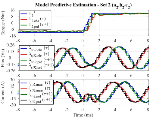
Fig. 12. Fast torque transient from 150% rated torque in motoring to 150% rated torque in generation at -6000 rpm, Set 2. From top to bottom: reference, observed and predicted torque (Nm); reference, observed and predicted stator flux (Vs); measured and predictedds-axis current (A); reference, measured and
predictedqs-axis current (A).
The motor position has been measured with an encoder. The power converter consists of two independent three-phase inverter IGBT power modules fed by a single DC power source of 550V. The digital controller is the dSpace DS1103 development board. The sampling frequency and the inverters switching frequency have been set at 6 kHz. The experimental results are related to the drive operation with torque control and speed control.
A. Torque Control
[image:7.595.310.559.292.487.2]The machine has been tested with a negative speed of -6000 rpm (2 pole pairs, about 200 Hz of electrical frequency) imposed by the prime mover (speed controlled), while the machine is torque controlled. The experimental results are related to the drive operation in healthy and open winding fault conditions.
Fig. 13. Fast torque transient from 150% rated torque in motoring to 150% rated torque in generation at -6000 rpm, Set 1. From top to bottom: reference, observed and predicted torque (Nm); (,) observed and predicted stator fluxes (Vs); (,) measured and predicted currents (A).
Fig. 14. Fast torque transient from 150% rated torque in motoring to 150% rated torque in generation at -6000 rpm, Set 2. From top to bottom: reference, observed and predicted torque (Nm); (,) observed and predicted stator fluxes (Vs); (,) measured and predicted currents (A).
1) Torque control under healthy conditions
The drive has been tested for both motoring and generating operation. A fast reference torque transient (40Nm/ms) from -24 Nm to +24 Nm (150% of the rated value) has been imposed for a speed of -6000 rpm and the results are shown in Figs.11-14. Each stator set will produce half of the total machine torque.
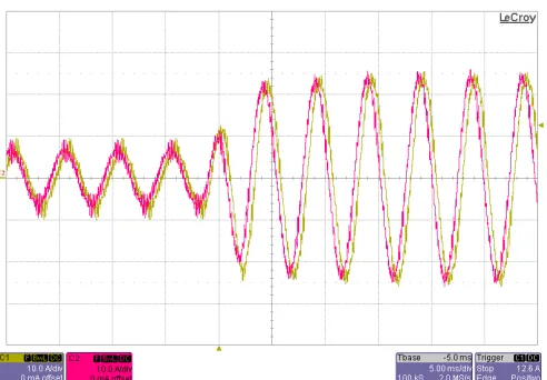
[image:7.595.42.282.302.496.2]Fig. 15. Fast torque transient from no-load up to 150% rated torque (24Nm) at -6000 rpm. Ch1:isa1(10A/div), Ch2:isa2(10A/div), Time scale: 5ms/div.
Fig. 16. Inverter 2 shut off during generation mode at -6000rpm and 10Nm. Ch1:isa1(10A/div), Ch2:isa2(10A/div), Time scale: 5ms/div.
It can be clearly noted in Figs.11 and 12 the one-step ahead prediction of currents and stator fluxes, as well as the deadbeat torque response, despite the high slew-rate of the torque reference that corresponds to an inversion of the mechanical power from -15kW to 15kW (150% rated value) in just 1.2ms.
The results shown in Figs 13,14 related to the (,) current and flux components demonstrate that the MPC scheme is stable and it works properly with a sampling frequency of 6 kHz.
The two three-phase current sets are balanced at both no-load and load-conditions, as can be seen in Fig. 15 that shows the machine currentsisa1andisa2for a step reference torque transient
from zero up to 24 Nm (150% of the rated value). The flux observer gainsgkfor all three-phase units have been set at 125 rad/s, corresponding to a frequency of 20 Hz.
[image:8.595.41.286.248.421.2]2) Fault ride-through capabiliy for open three-phase set The control “fault ride-through” capability when one inverter unit is suddenly disabled is shown in Figs. 16-18 (inverter 2 off) for generation operation at -6000 rpm and 10 Nm. The healthy unit exhibits sinusoidal current that increases within the allowed limits with the attempt at keeping the same torque and machine flux. The torque response and the qs-axis current response of the healthy set exhibit slight overshoots due to turn-off dynamics of the faulty set.
Fig. 17. Inverter 2 shut off during generation mode at -6000rpm and 10Nm, Set 1. From top to bottom: reference, observed and predicted torque (Nm); reference, observed and predicted stator flux (Vs); measured and predicted
ds-axis current (A); reference, measured and predictedqs-axis current (A).
Fig. 18. Inverter 2 shut off during generation mode at -6000rpm and 10Nm, Set 2. From top to bottom: reference, observed and predicted torque (Nm); reference, observed and predicted stator flux (Vs); measured and predictedds
-axis current (A); reference, measured and predictedqs-axis current (A).
In fact, the current transient of the faulty set is slow and acts as disturbance on the predictive algorithm. Nevertheless, this test is the proof of the modularity of the MS-based control schemes, with the maximum degree of freedom in the control of the single three-phase sets.
B. Closed Loop Speed Control
[image:8.595.313.553.299.491.2]Fig. 19. Speed control with inertial load from 0 to 6000 rpm, Set 1. From top to bottom: reference, observed and predicted stator flux (Vs); measured and predictedds-axis current (A); reference, measured and predictedqs-axis current
(A), maximum and observed load angle (deg).
Fig. 20. Speed control with inertial load from 0 to 6000 rpm, Set 2. From top to bottom: reference, observed and predicted stator flux (Vs); measured and predictedds-axis current (A); reference, measured and predictedqs-axis current
(A), maximum and observed load angle (deg).
Without any voltage limitation, the torque is limited only by the power converter current limit (24A). The flux-weakening becomes active for a speed that is near to 3000 rpm. The torque reduction is approximately proportional with the increment of the speed. The stator flux and stator currents of the single sets are perfectly controlled, as shown in Figs. 19,20.
[image:9.595.42.282.56.252.2]The MTPV limitation becomes active when the maximum load angle is reached, at a speed of about 4500 rpm. For safety, the maximum load angle has been set at 40 electrical degrees to avoid pull-out. As can be seen in Figs. 19, 20, at MTPV operation the load angle is properly limited at the reference value while the torque reduction is inversely proportional with the square of speed, as shown in Figs. 21, 22.
Fig. 21. Speed control with inertial load from 0 to 6000 rpm. From top to bottom: reference and estimated speed (krpm); reference, observed total and single sets torque (Nm); estimated total and single sets mechanical power (kW).
Fig. 22. Maximum torque per speed profile with 275V of DC source and 24A of power converter maximum current. Observed torque during the speed control test from 0 to 6000rpm.
The results presented at flux weakening with speed loop control clearly demonstrates that the proposed scheme is able to work properly under MTPV conditions with load angle limitation. The maximum motor fundamental frequency during the tests was 200 Hz with a ratio between the sampling frequency (6 kHz) and the fundamental frequency equal to 30.
VI. CONCLUSION
The paper proposes a dead-beat MPC for multiphase
induction machine configured as multiple three-phase
structures. The predictive algorithm is implemented on the basic structure of the Direct Flux Vector Control (DFVC) scheme for simultaneous flux and torque control without tuning. The dead-beat approach obtains very good dynamic control performance while keeping sinusoidal the machine currents.
[image:9.595.311.556.309.385.2] [image:9.595.44.282.314.508.2]APPENDIX
The Table I reports the machine main parameters. TABLE I.CHARACTERISTICS OF THE MACHINE UNDER TEST
Main Data
Rated phase voltage 230 Vrms
Rated power 10 kW
Overload capability 150% 5 min
Rated parameters@25C
Pole pairs p 2
Stator resistance Rs 289 mΩ Stator leakage inductance Lls 1.88 mH Magnetizing inductance Lm 15.7 mH Rotor resistance Rr 181 mΩ Rotor leakage inductance Llr 0.94 mH Rated stator fluxλs 0.23 Vs
REFERENCES
[1] P. Correa, M. Pacas, J. Rodrìguez, “Predictive Torque Control for Inverter-Fed Induction Machines”,IEEE Trans. Ind. Electron., vol. 54, no. 2, 2007, pp. 1073-1079.
[2] M.Preindl, S. Bolognani, “Model Predictive Direct Torque Control with Finite Control Set of PMSM Drive Systems, Part 1&2”,IEEE Trans. Ind. Informatics, vol. 9, no. 4 & no. 2, 2013, pp. 1912-1921 & pp. 648-657. [3] B. Boazzo, G. Pellegrino, “Model-Based Direct Flux Vector Control of
Permanent-Magnet Synchronous Motor Drives”,IEEE Trans. Ind. Appl.., 2015, vol. 51, no. 4, pp. 3126-3136.
[4] Y. Zhang, H. Yang, “Model Predictive Torque Control of Induction Motor Drives With Optimal Duty Cycle Control”,IEEE Trans. Power Elect., vol. 29, no. 12, 2014, pp. 6593-6603.
[5] C. A. Rojas, J. Rodríguez, F. Villarroel, J. R. Espinoza, C. A. Silva, M. Trincado, “Predictive Torque and Flux Control Without Weighting Factors”,IEEE Trans. Ind. Elect., 2013, vol. 60, no. 2, pp. 681-590. [6] S. A. Odhano, A. Formentini, P. Zanchetta, R. Bojoi, A. Tenconi, “Direct
Flux and Current Vector Control for Induction Motor Drives Using Model Predictive Control Theory”,IET Elec. Power Appl., vol. 11, no. 8, 2017, pp. 1483-1491.
[7] E. Levi, “Multiphase Electric Machines for Variable-Speed
Applications”,IEEE Trans. Ind. Electron., vol. 55, no. 5, pp. 1893-1909, 2008.
[8] E. Levi, “Advances in Converter Control and Innovative Exploitation of Additional Degrees of Freedom for Multiphase Machines”,IEEE Trans. Ind. Electron., Vol. 63, Issue 1, 2016, pp. 433-448.
[9] E. Jung, H. Yoo, S. Sul, H. Choi and Y. Choi, “A nine-phase permanent-magnet motor drive system for an ultrahigh-speed elevator,”IEEE Trans. Ind. Appl., vol. 48, no. 3, pp. 987-995, 2012.
[10] Z.Xiang-Jun, Y. Yongbing, Z. Hongtao, L. Ying, F. Luguang, and Y. Xu, “Modelling and control of multi-phase permanent magnet synchronous generator and efficient hybrid 3L-converters for large-drive wind turbines”, IET Electr. Power Appl., 2012, Vol.6, Issue 6, pp. 322-331. [11] W. Cao, B. Mecrow, G. Atkinson, J. Bennett, and D. Atkinson, “Overview
of Electric Motor Technologies Used for More Electric Aircraft (MEA)”,
IEEE Trans. Ind. Electron., 2011, vol. 59, no. 9, pp. 3523-3531. [12] M.G. Simões, P. Vieira, “A High-Torque Low-Speed Multiphase
Brushless Machine – A Perspective Application for Electric Vehicles”,
IEEE Trans. Ind. Electron.,Vol.49, No.5, pp. 1154–1164, 2002.
[13] Y. Burkhardt, A. Spagnolo, P. Lucas, M. Zavesky, P. Brockerhoff, “Design and analysis of a highly integrated 9-phase drivetrain for EV applications”, IEEE-ICEM, pp. 450–456, 2014.
[14] N. Schofield, X. Niu, O. Beik, “Multiphase Machines for Electric Vehicle Traction”, IEEE-ITEC, 2014.
[15] R. Bojoi; A. Cavagnino; M. Cossale; and A. Tenconi, “Multiphase Starter Generator for a 48-V Mini-Hybrid Powertrain: Design and Testing”,
IEEE Trans. Ind. Applicat., 2016, Vol. 52, Issue 2, pp. 1750 – 1758. [16] J. W. Kelly, E. G. Strangas, and J. M. Miller, “Multi-phase inverter
analysis”, Conf. Rec. IEEE-IEMDC, 2001, pp. 147–155.
[17] Y. Zhao and T.A. Lipo, “Space vector PWM control of dual three-phase induction machine using vector space decomposition”,IEEE Trans. Ind. Appl.., 1995, vol. 31, no. 5, pp. 1100-1108.
[18] F. Barrero, J. Prieto, E. Levi, R. Gregor, S. Toral, M.J. Duran, and M.
Jones, “An Enhanced Predictive Current Control Method for
Asymmetrical Six-Phase Motor Drives”, IEEE Trans. Ind.
Electron.,2011, vol. 58, no. 8, pp. 3242-3252.
[19] J.A. Riveros, F. Barrero, E. Levi, M.J. Duran, S. Toral, and M. Jones, “Variable-Speed Five-Phase Induction Motor Drive Based on Predictive Torque Control”,IEEE Trans. Ind. Electron., Vol. 60, No.8, 2013, pp. 2957-2968.
[20] Y. Wang, S. Tobayashi, and R.D. Lorenz, “A Low-Switching-Frequency Flux Observer and Torque Model of Deadbeat–Direct Torque and Flux Control on Induction Machine Drives”,IEEE Trans. Ind. Applicat., vol. 51, no. 3, 2015, pp. 2255-2267.
[21] S. Rubino, R. Bojoi, S.A. Odhano, and P. Zanchetta, “Model predictive direct flux vector control of multi-three phase induction motor drives”, Conf. Rec. IEEE Energy Conversion and Exposition (ECCE), 2017, pp.3633-3640.
[22] R.H. Nelson and P.C. Krause, “Induction machine analysis for arbitrary displacement beween multiple winding sets",IEEE Trans. Power Appl. and Systems, vol. PAS-93, 1974, pp. 841-848.
[23] S. Rubino, R. Bojoi, A Cavagnino, and S. Vaschetto, “Asymmetrical Twelve-Phase Induction Starter/Generator for More Electric Engine in Aircraft”, Conf. Rec. IEEE-ECCE, 2016, pp. 1-8.
[24] R. Bojoi, S. Rubino, A. Tenconi, S. Vaschetto, “Multiphase electrical machines and drives: A viable solution for energy generation and transportation electrification“, EPE 2016, pp. 632 – 639.
[25] G. Pellegrino, R. Bojoi, and P. Guglielmi, “Unified Direct-Flux Vector Control for AC Motor Drives”,IEEE Trans. Ind. Appl., 2011, vol. 47, no. 5, pp. 2093-2102.
[26] R. Bojoi, A. Cavagnino, A. Tenconi and S. Vaschetto, “Control of Shaft-Line-Embedded Multiphase Starter/Generator for Aero-Engine”,IEEE Trans. Ind. Electron., vol. 63, no.1, 2016, pp.641-652.
[27] P.L. Jansen and R.D. Lorenz, “A Physically Insightful Approach to the Design and Accuracy Assessment of Flux Observers for Field Oriented Induction Machine Drives”,IEEE Trans. Ind. Appl., vol. 30, no.1, pp. 101-110, 1994.
[28] R. Bojoi, E. Armando, G. Pellegrino, and S.G. Rosu, “Self-commissioning of inverter nonlinear effects in AC drives”, Conf. Rec. IEEE ENERGYCON, 2012, pp. 213-218.
[29] R. Bojoi, A. Tenconi and S. Vaschetto, "Direct Stator Flux and Torque Control for asymmetrical six-phase induction motor drives",2010IEEE ICIT, 2010, pp. 1507-1512.