1
An efficient algorithm for exact computation of system and survival signatures
using binary decision diagrams
Sean Reed
Resilience Engineering Research Group, University of Nottingham, University Park, Nottingham NG7 2RD, UK
Abstract
System and survival signatures are important and popular tools for studying and analysing the reliability of systems. However, it is difficult to compute these signatures for systems with complex reliability structure functions and large numbers of components. This paper presents a new algorithm that is able to compute exact signatures for systems that are far more complex than is feasible using existing approaches. This is based on the use of reduced order binary decision diagrams (ROBDDs), multidimensional arrays and the dynamic programming paradigm. Results comparing the computational efficiency of deriving signatures for some example systems (including complex benchmark systems from the literature) using the new algorithm and a comparison enumerative algorithm are presented and demonstrate a significant reduction in computation time and improvement in scalability with increasing system complexity.
Keywords
system signature, survival signature, binary decision diagram, system reliability
Notation
𝑚 Number of components in the system
𝐾 Number of component types in the system, where components of the same type have exchangeable random failure times
𝑀𝑘 Number of components of type k
𝑥𝑖 Boolean variable representing the state of component 𝑖 where 𝑥𝑖 = 1 if the component functions and 𝑥𝑖 = 0 if the component is failed
𝑥 Vector of length m representing the system component states where the value at index 𝑖 ∈ {1, … , 𝑚} corresponds to 𝑥𝑖
𝜙 Boolean function representing the system reliability structure where 𝜙(𝑥) = 1 if the system functions with component state vector 𝑥 and 𝜙(𝑥) = 0 if the system is failed
𝑓𝑥𝑖=𝑣 Boolean function f evaluated with Boolean variable 𝑥𝑖 = 𝑣 𝑇𝑠 Random failure time of the system
𝑇𝑙:𝑚 lth order statistic for the random component failure times
𝑞𝑙 Probability that the system failure time coincides with the lth component failure (i.e. 𝑃(𝑇𝑠 = 𝑇𝑙:𝑚 )) 𝑞 Vector of length 𝑚 known as the system signature where the value at index 𝑙 ∈ {1, … , 𝑚} corresponds
2
𝑆𝑙1,…,𝑙𝐾 Set of state vectors for the m components that contain precisely 𝑙𝑘 functioning components of type k
|𝑆𝑙1,…,𝑙𝐾| Cardinality of 𝑆𝑙1,…,𝑙𝐾
𝑆 Multidimensional array with 𝐾 dimensions where the value at index (𝑙1, … , 𝑙𝐾) in dimensions (1, … , 𝐾) respectively corresponds to 𝑆𝑙1,…,𝑙𝐾
|𝑆| Multidimensional array with 𝐾 dimensions where the value at index (𝑙1, … , 𝑙𝐾) in dimensions (1, … , 𝐾) respectively corresponds to |𝑆𝑙1,…,𝑙𝐾|
Φ̅𝑙1,…,𝑙𝐾 Number of state vectors for the m components that both contain precisely 𝑙𝑘 functioning components of type k and result in the system functioning
Φ̅ Multidimensional array with 𝐾 dimensions where the value at index (𝑙1, … , 𝑙𝐾) in dimensions (1, … , 𝐾) respectively corresponds to Φ̅𝑙1,…,𝑙𝐾
Φ𝑙1,…,𝑙𝐾 Probability that the system functions given that exactly (𝑙1, … , 𝑙𝐾) components of types (1, … , 𝐾)
respectively function
Φ Multidimensional array with 𝐾 dimensions known as the survival signature where the value at index (𝑙1, … , 𝑙𝐾) in dimensions (1, … , 𝐾) respectively corresponds to Φ𝑙1,…,𝑙𝐾
𝐶𝑡𝑘 Number of components of type k in the system that function at time 𝑡 > 0 𝐹𝑘 Cumulative distribution function for the time to failure of components of type 𝑘 𝐴‡ The complement of multidimensional array A
𝐴 ⊕ 𝐵 Elementwise addition of multidimensional arrays A and B
𝐴 ⊖ 𝐵 Elementwise subtraction of multidimensional array A from multidimensional array B 𝐴 ⊘ 𝐵 Elementwise division of multidimensional array A from multidimensional array B
𝐴 ⊞ 𝑘 Resize-k operation on multidimensional array A 𝐴 ⊛ 𝑘 Shift-k operation on multidimensional array A
1
Introduction
The system signature, introduced by Samaniego [1], is a useful tool for studying the reliability of coherent systems [2]. Consider a coherent system of m components with independent identically distributed failure times. Let 𝑇𝑠 > 0 be the random failure time of the system and let 𝑇𝑗:𝑚 be the lth order statistic for the random component failure times with 𝑇1:𝑚 ≤ 𝑇2:𝑚 ≤ ⋯ ≤ 𝑇𝑚:𝑚. The system signature is defined as the vector 𝑞 where the value at index 𝑙 ∈ {1,2, … , 𝑚}, denoted 𝑞𝑙, gives the probability that the system failure time
coincides with the lth component failure
𝑞𝑙 = 𝑃(𝑇𝑠 = 𝑇𝑙:𝑚) (1)
3
similar to the system signature, fulfils the role of a quantitative model of the system reliability structure that is entirely separated from the random failure times of the components. The survival signature has the advantage that is can be easily generalised to systems with multiple types of components unlike the system signature for which this is practically impossible [6]. This generalisation represents a significant practical advantage since many systems contain multiple component types, including networks which contain at least two types of component (‘nodes’ and ‘links’). Let 𝑥 = (𝑥1, 𝑥2, … , 𝑥𝑚) ∈ {0,1} 𝑚 represent a Boolean state
vector for a system of m components with exchangeable failure times, where 𝑥𝑖 = 1 if component 𝑖 functions and 𝑥𝑖 = 0 if it is failed. Also let 𝜙: {0,1}𝑚 → {0,1} represent the system reliability structure function, defined for all 2𝑚 possible 𝑥, where 𝜙(𝑥) = 1 if the system functions with component states 𝑥 and 𝜙(𝑥) = 0 if it is failed. Finally, let 𝑆𝑙 denote the set of component state vectors with exactly l of the m components functioning (i.e. ∑𝑚𝑖=1𝑥𝑖 = 𝑙). The survival signature is then defined as the vector Φ where the value at index 𝑙 ∈ {0,1,2, … , 𝑚}, denoted Φ𝑙, gives the probability that the system functions given that precisely l components function
Φ𝑙= (𝑚𝑙 )−1∑ 𝜙(𝑥) 𝑥∈𝑆𝑙
(2)
Now consider the case where the m components in the system are partitioned into 𝐾 different types, where the 𝑀𝑘 components of type 𝑘 ∈ {1, … , 𝐾} have exchangeable random failure times. Let 𝑆𝑙1,…,𝑙𝐾 denote the set of component state vectors that contain precisely 𝑙𝑘 ∈ {0,1, … , 𝑀𝑘} functioning components of type k (i.e. those for which ∑𝑀𝑖=1𝑘 𝑥𝑖𝑘 =𝑙𝑘 for 𝑘 = 0,1, … , 𝐾 − 1 where 𝑥𝑖𝑘 is the ith component of type k). Also let |𝑆𝑙1,…,𝑙𝐾| = ∏ (𝑀𝑙𝑘
𝑘) 𝐾
𝑘=1 denote the cardinality of 𝑆𝑙1,…,𝑙𝐾 and Φ̅𝑙1,…,𝑙𝐾 = ∑𝑥𝜖𝑆𝑙0,…,𝑙𝐾−1𝜙(𝑥) denote the number
of state vectors from 𝑆𝑙1,…,𝑙𝐾 for which the system functions. The generalised survival signature, Φ, is then
defined as the multidimensional array with K dimensions where the value at index (𝑙1 ∈ {0, . . , 𝑀1}, … , 𝑙𝐾 ∈ {0, . . , 𝑀𝐾}) in dimensions (1, … , 𝐾) respectively, denoted Φ𝑙1,…,𝑙𝐾, gives the probability that the system
functions given that precisely (𝑙1, … , 𝑙𝐾) components of types (1, … , 𝐾) respectively function Φ𝑙1,…,𝑙𝐾 =
Φ̅𝑙1,…,𝑙𝐾
|𝑆𝑙1,…,𝑙𝐾|
(3)
Let 𝐶𝑡𝑘𝜖{0, … , 𝑀𝑘} denote the number of components of type k in the system that function at time 𝑡 > 0. The probability that the system functions at time 𝑡 can be calculated using the survival signature and the joint probability distribution for the number of functioning components of each type at time t
𝑃(𝑇𝑆 > 𝑡) = ∑ … 𝑀1
𝑙1=0
∑ [Φ𝑙1,…,𝑙𝐾𝑃 (⋂{𝐶𝑡𝑘 = 𝑙 𝑘} 𝐾
𝑘=1
)] 𝑀𝐾
𝑙𝐾=0
(4)
If failure times of components of type k are conditionally independent and identically distributed with CDF 𝐹𝑘(𝑡) and failure times of components of different types are independent, then
𝑃(𝑇𝑆 > 𝑡) = ∑𝑀𝑙11=0…∑ [Φ𝑙1,…,𝑙𝐾∏ ((
𝑀𝑘
𝑙𝑘) [𝐹𝑘(𝑡)]
𝑀𝑘−𝑙𝑘[1 − 𝐹𝑘(𝑡)]𝑙𝑘)
𝐾
𝑘=1 ]
𝑀𝐾
𝑙𝐾=0
(5)
For systems containing a single component type, the system signature and survival signature have the simple relation
4
Several theoretical applications of the survival signature to problems in the field of reliability engineering have already been published including nonparametric predictive inference for system reliability [7]; Bayesian inference for reliability of systems and networks [8]; modelling uncertain aspects of system dependability [9]; predictive inference for system reliability after common-cause component failures [10]; imprecise system reliability and component importance [11]; Bayesian nonparametric system reliability using sets of priors [12] and comparing systems with heterogeneous components [13].
Despite the advances is the theory and development of numerous application for signatures, practical applications have until now been limited to the analysis of relatively small problems. The main reason for this is that the computation of signatures using existing methods is difficult unless the number of components is small or the system reliability structure function is quite trivial [2,6]. The aim of this paper is to present a new and computationally efficient algorithm based on binary decision diagrams for computing exact system and survival signatures and report its computational efficiency for a number of example systems, including large and complex systems that have been derived from practice and were published as benchmarks in the literature. The remainder of this paper is organised as follows: Section 2 describes the existing methods that are available for the computation of system and survival signatures. Section 3 introduces the new algorithm. Section 4 presents some results on the efficiency of the new algorithm in computing system and survival signatures for a set of example systems, including some large and complex benchmark systems from the literature. Section 5 summarises the paper, gives some concluding remarks and also discusses limitations and areas for future work.
2
Existing Methods for System and Survival Signature Computation
A small number of methods for computing system signatures have been published in the literature and are based on minimal ordered cut sets, diagonal sections of the reliability structure function and generating functions. Kochar et al [14] note that the system signature can be defined for 𝑗 ∈ {1,2, … , 𝑚} as
𝑞𝑗 =
𝑛𝑢𝑚𝑏𝑒𝑟 𝑜𝑓 𝑐𝑜𝑚𝑝𝑜𝑛𝑒𝑛𝑡 𝑜𝑟𝑑𝑒𝑟𝑖𝑛𝑔𝑠 𝑓𝑜𝑟 𝑤ℎ𝑖𝑐ℎ 𝑡ℎ𝑒 𝑗𝑡ℎ 𝑓𝑎𝑖𝑙𝑢𝑟𝑒 𝑐𝑎𝑢𝑠𝑒𝑠 𝑠𝑦𝑠𝑡𝑒𝑚 𝑓𝑎𝑖𝑙𝑢𝑟𝑒
𝑚! (7)
The system signature can therefore be computed by generating the 𝑚! permutations of component orderings and counting the number of permutations for which the jth component failure results in system failure for 𝑗 ∈ {1,2, … , 𝑚}. The system failure evaluation might be carried out, for example, by deriving the minimal cut sets for the system and comparing them with subsets of increasing size from each component ordering permutation until a match is found. A subset of components from a system is a cut set if the failure of those components implies failure of the system and is a minimal cut set if it has no proper subset that is also a cut set. Since the computational expense of this approach grows approximately with the product of 𝑚! and the number of minimal cut sets, it is only feasible for simple systems. Boland [15] showed that the system signature for a system could also be defined for 𝑗 ∈ {1,2, … , 𝑚} as
𝑞𝑗 =
𝑛𝑢𝑚𝑏𝑒𝑟 𝑜𝑓 𝑚𝑖𝑛𝑖𝑚𝑎𝑙 𝑜𝑟𝑑𝑒𝑟𝑒𝑑 𝑐𝑢𝑡 𝑠𝑒𝑡𝑠 𝑜𝑓 𝑠𝑖𝑧𝑒 j 𝑚! ÷ (𝑚 − 𝑗)!
(8)
5
can be computed for a system from the diagonal section of the reliability structure function via derivatives. This method relies on complicated algebraic manipulations and is best suited to hand calculation with systems with small numbers of components. Triantafyllou and Koutras [17] presented an approach for computing the system signatures for linear and circular k-out-of-n: F systems using generating functions. Linear and circular k-out-of-n: F systems consist of linear and circularly arranged components, respectively, where the system fails if and only if at least k consecutive components fail. Whilst this method is computation efficient it is applicable only to the small subset of systems that can be modelled as a linear or circular k-out-of-n: F system such as certain telecommunication and pipeline networks. For systems that can be decomposed into disjoint subsystems, Marichal and Mathonet [16] and Da et al [18] derived formulas for computing the system signature of a system from the system signatures computed for its subsystems and the reliability structure function for the system in terms of its subsystems. This reduces the computational burden compared to computing the system signature for the complete system directly.
An enumerative approach can be used for the computation of the survival signature, where each possible state vector is evaluated in turn, such as the following approach used by the ReliabilityTheory package [19] for the R programming language [20]:
Derive the minimal cut sets for the system.
Generate each of the 2𝑚 possible component state vectors.
Compare each component state vector to the minimal cut sets to determine whether it results in the system functioning or not.
Count the number of component state vectors with (𝑙1, … , 𝑙𝐾) components of types (1, … , 𝐾)
functioning that result in system functioning to obtain Φ̅𝑙1,…,𝑙𝐾−1 for all ∏𝐾𝑘=1𝑀𝑘+ 1 different (𝑙1, … , 𝑙𝐾).
Obtain Φ𝑙1,…,𝑙𝐾 by dividing Φ̅𝑙1,…,𝑙𝐾 by |𝑆𝑙1,…,𝑙𝐾| for all ∏𝑘=1𝐾 𝑀𝑘+ 1 different (𝑙1, … , 𝑙𝐾).
However, the computational expense of this approach grows approximately with the product of 2𝑚 and the number of minimal cut sets, it becomes infeasible for complex systems (e.g. for 𝑚 = 30 there are over 1 billion possible component state vectors to consider).
In summary, the existing methods for computing system and survival signatures are only computationally feasible when applied to relatively simple systems with small numbers of components. If the system can be reduced to a set of disjoint subsystems, then the combinational formulas from Marichal and Mathonet [16] and Da et al [18] can be useful in reducing computational burden but do not address the challenge of deriving the signatures for the subsystems. The method from Triantafyllou and Koutras [17] is efficient but its applicability is limited to the small number of systems that can be modelled as linear or circular k-out-of-n: F systems. Therefore new methods are required to enable the practical computation of system and survival signature for many large and complex real world systems.
3
Description of New Method for System and Survival Signature Computation based on
Binary Decision Diagrams
A new algorithm for efficiently computing system and survival signatures is presented in this section. The algorithm utilises reduced ordered binary decision diagrams (hereafter referred to as BDD) and multidimensional array data structures in the signature computation process.
3.1 Reduced Ordered Binary Decision Diagram (BDD) Data Structure
6
𝑓 = ((𝑥𝑖 = 1) ∧ 𝑓𝑥𝑖=1) ∨ ((𝑥𝑖 = 0) ∧ 𝑓𝑥𝑖=0) (9)
where 𝑓𝑥𝑖=𝑣 is 𝑓 evaluated with 𝑥𝑖 = 𝑣.
Each BDD contains two terminal nodes that represent the Boolean constant values 1 and 0. Each non-terminal node represents a subfunction g, is labelled with a Boolean variable v and has two outgoing edges. By applying a total ordering on the m Boolean variables for function f by mapping them to the integers 0, … , 𝑚 − 1, and applying the Shannon decomposition recursively to f, it can be represented as a binary tree with m+1 levels. Each intermediate node, referred to as an if-then-else (ite) node, at level 𝑙 ∈ {0, … , 𝑚 − 1}(where the root node is at level 0 and the nodes at level 𝑚 − 1 are adjacent to the terminal nodes) represents a Boolean function g on variables 𝑥𝑙,𝑥𝑙+1, … , 𝑥𝑚−1. It is labelled with variable 𝑥𝑙 and has two out edges called 1-edge
and 0-edge linking to nodes labelled with variables higher in the ordering. 1-edge corresponds to 𝑥𝑙 = 1 and links to the node representing 𝑔𝑥𝑙=1, whist 0-edge corresponds to 𝑥𝑙 = 0 and links to the node representing
𝑔𝑥𝑙 =0. In addition, the following two reduction rules are applied:
1. Isomorphic subgraphs are merged.
2. Any node whose two children are isomorphic is eliminated.
Complement edges [23] are an extension to standard BDDs that reduce size and computation time. A complement edge is an ordinary edge that is marked to indicate that the connected child node (at a higher level) is to be interpreted as the complement of its Boolean function. The use of complement edges is limited to the 0-edges to ensure canonicity. In general, the BDD representation of a Boolean function of m variables has far fewer nodes than 2𝑚 nodes.
Efficient algorithms have been developed for the computation of the BDD representation of the reliability structure function of a system from fault trees [24], event trees [25], networks [26] and dynamic flowgraphs [27]. The chosen variable ordering often has a significant impact on the size of the resultant BDD. Finding the optimum variable ordering is known to be a NP-hard problem [28], however many efficient heuristic methods have been developed (e.g. for fault trees [29] or networks [30]).
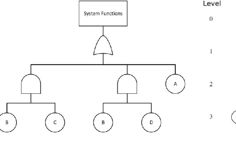
An example of a success tree (i.e. logical complement of a fault tree, where basic events and the top event represent component and system functioning respectively) is shown in Figure 1a. Figure 1b shows a complemented edge BDD representation of the success tree, where components are ordered 𝐴 < 𝐵 < 𝐶 < 𝐷,
7
Figure 1a - A success tree from an example system. Figure 1b – A complemented edge BDD representation of the success tree shown
in Figure 1a.
3.2 Computational representation of Φ and Φ̅
The number of possible values for Φ𝑙1,…,𝑙𝐾 or Φ̅𝑙1,…,𝑙𝐾 from Eqn. 3 for any (𝑙1, … , 𝑙𝐾), across all possible systems with K component types and 𝑀𝑘 components of type k, is given by ∏ (𝑚𝑎𝑥 ((⌈𝑀𝑀𝑘
𝑘÷ 2⌉) , ( 𝑀𝑘
⌊𝑀𝑘÷ 2⌋))) 𝐾
𝑘=1 . Thus the range of possible values can be very large for systems
with many components and component types and require high bit length numerical data structures to represent computationally to exact or high precision. Additionally there are a total of ∏𝐾𝑘=1𝑀𝑘+ 1 different (𝑙1, … , 𝑙𝐾) indices for which Φ𝑙1,…,𝑙𝐾 and Φ̅𝑙1,…,𝑙𝐾 from Eqn. 3 need to be computed. These values can be represented
computationally using a multidimensional array data structure with K dimensions and length 𝑀𝑘+ 1 in dimension k, where the value stored at index (𝑙1, … , 𝑙𝐾) of the array is equal to Φ𝑙1,…,𝑙𝐾 or Φ̅𝑙1,…,𝑙𝐾. Across all possible systems with m components and K component types, the maximum possible value for ∏𝐾𝑘=1𝑀𝑘+ 1
is (𝑚𝐾+ 1)
𝐾
. Therefore, the computational representation of Φ̅ or Φ for systems with many components and component type can require significant amount of memory. For example, the computational representation of the survival signature for a 50 component system partitioned evenly across 10 component types would require the use of a multidimensional array with 60,466,176 elements and 24 bits of memory per element to ensure exact representation of Φ̅ or Φ – a total of over 180 megabytes of memory.
3.3 New algorithm for calculating system and survival signatures
A new efficient algorithm that outputs a multidimensional array representation of the survival signature, Φ, for a system is presented in this section. For the case of a single component type, i.e. K=1, an array representing the system signature 𝑞 can be derived from the array representing the survival signature Φ by applying the simple transformation given in Eqn. 6. The inputs to the algorithm are:
8
labelled with Boolean variable 𝑥𝑖 representing the state of component i in the ordering, 1-edges from a node represent survival of the labelling component, 0-edges from a node represent failure of the labelling component, the terminal 1 node represents system survival and the terminal 0 node represents system failure.
An associative array [31] (also known as a map or dictionary data type) that associates each of the m
components in the system with its component type from {1, … , 𝐾}.
The algorithm computes multidimensional arrays representing Φ̅ for nodes at successively lower levels of the BDD, starting with the terminal nodes at level m and finishing with the root node. The array representing Φ̅ for each ite node is computed using the results from its two child nodes, representing the positive and negative sub-parts of the Shannon decomposition of the Boolean function represented by the node (see Eqn. 9). These result are stored in an associative array and retrieved whenever the node is reencountered during the computation process. The algorithm therefore follows the dynamic programming paradigm [32] in which a problem is solved by identifying a collection of sub-problems, solving each sub-problem using the solutions to its problems, iteratively solving the problems in order of increasing size and storing the sub-problem solutions and then retrieving them instead of resolving them when shared sub-sub-problems are reencountered. An array representing the survival signature Φ is then computed by normalising the array representing Φ̅ for the complete BDD using an array representing |𝑆|.
One unary operation and five binary operations and on multidimensional arrays will now be defined that are used in the algorithm. The unary operation on an array is named here as the complement operation and is only required where complement BDDs are used. The complement operation on array A, denoted 𝑋‡, outputs an array B where the value at each index (𝑙1, … , 𝑙𝐾) is equal to ∏ (𝐿𝑘𝑙− 1
𝑘 )
𝐾
𝑘=1 minus the value at that index in
array A, where 𝐿𝑘 is the length of array A in dimension k. The first three binary operations are defined for pairs of multidimensional arrays with the same number of dimensions and dimension lengths. They are named here as the elementwise addition, elementwise subtraction and elementwise division operations. The elementwise addition of two arrays A and B, denoted 𝐴 ⊕ 𝐵, outputs an array C with the same number of dimensions and dimension lengths as arrays A and B where the value at each index in array C is equal to the sum of the values at the same index in arrays A and B. Elementwise subtraction of array B from array A, denoted 𝐴 ⊖ 𝐵, outputs an array C with the same number of dimensions and dimension lengths as arrays A
and B where the value at index each index in array C is equal to the value at that index in array A minus the value at that index in array B. Elementwise division of array A by array B, denoted 𝐴 ⊘ 𝐵, outputs an array
C with the same number of dimensions and dimension lengths as arrays A and B where the value at index in array C is equal to the value at that index in array A divided by the value at that index in array B. The final two binary operations are defined for a first argument of a multidimensional array with K dimensions and a second argument of an integer 𝑘 ∈ {1, … , 𝐾}. They are named here as the resize-k and shift-k operations. The resize-k operation on array A by integer k is denoted 𝐴 ⊞ 𝑘. It returns an array B with the same number of dimensions and dimension lengths as A, except with the length of dimension k increased by 1 to length 𝐿, where:
the value in B at each index (𝑙1, … , 𝑙𝑘, … , 𝑙𝐾), except where 𝑙𝑘 = 𝐿, is equal to the value from A at the same index.
the value in B at each index (𝑙1, … , 𝐿, … , 𝑙𝐾) is equal to 0.
The shift-k operation on array A by integer k is denoted 𝐴 ⊛ 𝑘. It returns an array B with the same number of dimensions and dimension lengths as A, except with the length of dimension k increased by 1, where:
9
the value in B at each index (𝑙1, … ,0, … , 𝑙𝐾) is equal to 0.
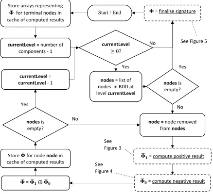
The main routine of the algorithm is shown in Figure 2. Arrays representing Φ̅ for the terminal nodes are computed first. A BDD comprising of only the terminal 1 node represents a Boolean function on 0 components of each type that evaluates to 1 (i.e. system survival). Therefore the array representing Φ̅ for the terminal 1 node has K dimensions of length 1 and a single element of 1. Conversely, a BDD comprising of only a terminal 0 node represents a Boolean function on 0 components of the K components type that evaluates to 0 (i.e. system failure). Therefore the array representing Φ̅ for the terminal 0 node has K dimensions of length 1 and a single element of 0. For example, the arrays representing Φ̅ for the terminal 1 and terminal 0 nodes from the BDD in Figure 1b, which corresponds to a system with two component types (i.e. K=2) with the success tree depicted in Figure 1a, are [[1]] and [[0]] respectively. The results for Φ̅ corresponding to the terminal nodes are then stored in an associative array that represents a cache of all computed node results.
10
Figure 2 – Main routine of the algorithm that computes survival signatures.
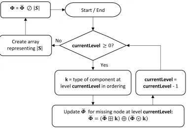
Once the array representing Φ̅ for the root node in the BDD has been computed, the subroutine shown in Figure 5 is used to update the array to account for remaining levels in the BDD, i.e. where the root node is at a level greater than 0, and obtain the survival signature through application of a normalisation step. Due to the removal of isomorphic child nodes in the BDD construction process, a root node at a level greater than 0 signifies that the survival or failure of the components at lower levels in the ordering do not influence whether or not the system survives. Updating the array representing Φ̅ to account for such levels follows the same process as for levels skipped in the edge path between an ite node and its child node. For the purpose of normalisation, an array representing |S| is created with K dimensions and length 𝑀𝑘+1 in dimension k, with the value at each index (𝑙1, … , 𝑙𝑘, … , 𝑙𝐾) set equal to ∏ (𝑀𝑙𝑘
𝑘) 𝐾
𝑘=1 . Elementwise division of the array
representing Φ̅ by the array representing |S| is then performed to derive the array representing the survival signature Φ, which is the final result output by the algorithm.
No Yes
No Yes
No
Yes Start / End Store arrays representing
𝚽̅ for terminal nodes in cache of computed results
𝚽 = finalise signature
currentLevel = number of
components - 1
currentLevel ≥ 0?
nodes = list of
nodes in BDD at level currentLevel
nodes is
empty?
nodes is
empty?
currentLevel = currentLevel - 1
Store 𝚽̅ for node node in cache of computed results
node = node removed
from nodes
𝚽̅ = 𝚽̅𝟏 ⨁ 𝚽̅𝟎
𝚽̅𝟏 = compute positive result
𝚽̅𝟎 = compute negative result See Figure 5
See Figure 3
11
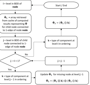
Figure 3 – “compute positive result” subroutine of the algorithm that computes 𝚽̅ for positive part of Shannon decomposition of an ite node.
No
Yes
Start / End
𝚽̅𝟏 = array retrieved
from cache of computed results representing 𝚽̅ for child node connected
to 1-edge of node node
i = level in BDD of node
node
j = level in BDD of child
node connected to 1-edge of node node
j > i + 1?
Update 𝚽̅𝟏 for missing node at level j -1:
𝚽̅𝟏 = (𝚽̅𝟏⊞ 𝐤) ⊕ (𝚽̅𝟏⊛ 𝐤)
k = type of component at
level j – 1 in ordering
j = j - 1
k = type of component at
12
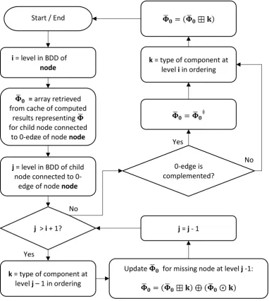
Figure 4 – “compute negative result” subroutine of the algorithm that computes 𝚽̅ for negative part of Shannon decomposition of an ite node.
No
Yes
No Yes
Start / End
𝚽̅𝟎 = array retrieved
from cache of computed results representing 𝚽̅ for child node connected
to 0-edge of node node
i = level in BDD of node
node
j = level in BDD of child
node connected to 0-edge of node node
0-edge is complemented?
j > i + 1?
Update 𝚽̅𝟎 for missing node at level j -1:
𝚽̅𝟎 = (𝚽̅𝟎⊞ 𝐤) ⊕ (𝚽̅𝟎⊛ 𝐤)
k = type of component at
level j – 1 in ordering
j = j - 1 𝚽̅𝟎= 𝚽̅𝟎‡
k = type of component at
13
Figure 5 – “finalise signature” subroutine of the algorithm that finalises the computation of a survival signature.
A
-type 1
E –
type 1
B –
type 2
D –
type 2
C –
[image:13.595.343.523.372.684.2]type 2
Figure 6a – Reliability block diagram for an example five component system with two component types, where each node is labelled with the component and component type.
Figure 6b – BDD for the example system shown in Figure 6a, where each ite node is labelled with
the component and node number.
Yes No
Start / End
currentLevel ≥ 0?
Update 𝜱̅ for missing node at level currentLevel: 𝚽̅ = (𝚽̅ ⊞ 𝐤) ⊕ (𝚽̅ ⊛ 𝐤)
k = type of component at
level currentLevel in ordering
currentLevel = currentLevel - 1 𝚽 = 𝚽̅ ⊘|𝑺|
Create array representing |𝐒|
14
3.4 Example Computation
Consider a five component system (consisting of components A, B, C, D and E) with two component types (consisting of types 1 and 2) and the reliability structure given by the reliability block diagram shown in Figure 6a, where each node is labelled with the component and component type. The corresponding BDD constructed with components ordered alphabetically is shown in Figure 6b, where each ite node is labelled with the component and node number.
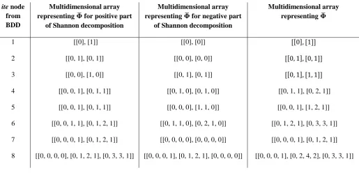
[image:14.595.42.558.207.458.2]The multidimensional arrays representing Φ̅ for the terminal 1 and terminal 0 nodes of this system are [[1]] and [[0]] respectively. The multidimensional arrays representing Φ̅ for each of the ite nodes in the BDD are given in Table 1.
Table 1 - Multidimensional arrays representing 𝚽̅ for each ite node from the BDD shown in Figure 6b.
ite node
from BDD
Multidimensional array representing 𝚽̅ for positive part
of Shannon decomposition
Multidimensional array representing 𝚽̅ for negative part
of Shannon decomposition
Multidimensional array representing 𝚽̅
1 [[0], [1]] [[0], [0]] [[0], [1]]
2 [[0, 1], [0, 1]] [[0, 0], [0, 0]] [[0, 1], [0, 1]]
3 [[0, 0], [1, 0]] [[0, 1], [0, 1]] [[0, 1], [1, 1]]
4 [[0, 0, 1], [0, 1, 1]] [[0, 1, 0], [0, 1, 0]] [[0, 1, 1], [0, 2, 1]]
5 [[0, 0, 1], [0, 1, 1]] [[0, 0, 0], [1, 1, 0]] [[0, 0, 1], [1, 2, 1]]
6 [[0, 0, 1, 1], [0, 1, 2, 1]] [[0, 1, 1, 0], [0, 2, 1, 0]] [[0, 1, 2, 1], [0, 3, 3, 1]]
7 [[0, 0, 0, 1], [0, 1, 2, 1]] [[0, 0, 0, 0], [0, 0, 0, 0]] [[0, 0, 0, 1], [0, 1, 2, 1]]
8 [[0, 0, 0, 0], [0, 1, 2, 1], [0, 3, 3, 1]] [[0, 0, 0, 1], [0, 1, 2, 1], [0, 0, 0, 0]] [[0, 0, 0, 1], [0, 2, 4, 2], [0, 3, 3, 1]]
The array representing |𝑆| is:
|𝑆| = [[1, 3, 3, 1], [2, 6, 6, 2], [1, 3, 3, 1]]
Finally, the multidimensional array representation of the survival signature Φ for the BDD obtained through elementwise division of the array representing Φ̅ for the BDD (i.e. the result for the root node of the BDD, ite
node 8, given from Table 1) by the array representing|𝑆| is:
Φ = [[0, 0, 0, 1], [0, 2, 4, 2], [0, 3, 3, 1]] ⊘ [[1, 3, 3, 1], [2, 6, 6, 2], [1, 3, 3, 1]] = [[0, 0, 0, 1], [0,13,23, 1] , [0, 1, 1, 1]]
4
Application of New Method for System and Survival Signature to Benchmark Problems
The algorithm presented in this paper has been implemented as a computer code (available on request) in the Python programming language, using the NumPy open source library [33] to provide an efficient implementation of multi-dimensional arrays and array operations. The algorithm and its implementation were validated for correctness by verifying computed signatures for a set of small network reliability problems (which contained 22 components or less) against results obtained from the ReliabilityTheory package [19] for the R programming language [20]. Additional verification was performed by using Eqn. 5 to calculate the probabilities of system survival from the computed survival signatures and comparing them against the known values for each system.15
were composed by the author, whilst the European 1 and European 3 systems were obtained from the literature [34] and have been used previously by other researchers as benchmarks [24]. European 1 and European 3 systems were chosen since they are large and complex systems derived from practice that feature many cut-sets (46188 and 24386 respectively) and components (61 and 80 respectively). Finally, two further systems named European 1a and European 1b were derived from the European 1 system by reducing the number of component types (from the original 14 types to 3 and 6 respectively). The fault tree and component types for system 1 are given in Table A.1 and Table A.2, respectively, of Appendix A. A BDD for each of the seven fault trees was computed using the method from Rauzy [24] with components ordered according to the sequence in which they were first encountered during a depth first traversal [35] of the fault tree starting at the top event.
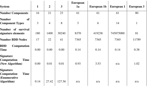
[image:15.595.62.540.308.593.2]Table 3 presents the results for computing signatures for each of the example systems, using both the new algorithm that was presented in Section 3 and an enumerative algorithm similar to that described in Section 2. The results were obtained using a computer with an Intel i3-4130 3.4GHz CPU and 8GB RAM. In Appendix B, the survival signature that was computed for system 1 is shown in Table B.1a and Table B.1b, whilst the system signature for the European 3 system is shown in Table B.2.
Table 3 – Results for computing signatures using new algorithm and enumerative algorithm for example systems (all times given in seconds)
System 1 2 3
European
1a European 1b European 1 European 3
Number Components 16 21 23 61 61 61 80
Number of
Component Types 3 4 8 3 6 14 1
Number of survival
signature elements 180 1400 30240 8370 419238 745875000 81
Number BDD Nodes 17 22 41 7365 7365 7365 11789
BDD Computation
Time 0.00 0.00 0.00 0.14 0.14 0.14 0.38
Signature
Computation Time
(New Algorithm) 0.00 0.01 0.01 0.93 3.53 n/a 1.02
Signature
Computation Time (Enumerative
Algorithm) 0.14 27.42 127.56 n/a n/a n/a n/a
16
was for the full European fault tree 1 with all 14 component types. For this system, the array representation of the survival signature has over 0.75 billion elements and the memory required to represent it in RAM exceeded the resources available on the computer used to perform the analysis.
5
Summary and Conclusions
The system signature and survival signature are valuable tools for the analysis and assessment of system reliability as evidenced by the wide range of theoretical applications found in the literature. These applications include comparing the reliability of different system designs and determining where redundancy should be added to a system to maximise gains in reliability. It is well known that the computation of signatures is very challenging and the previously published approaches are only feasible for simple systems with few components. The development of algorithms that are able to compute signatures for complex systems with large numbers of components is therefore important so that they can be analysed with the many signature based reliability analysis methods that have been published in the literature.
A new algorithm for computing system and survival signatures was introduced, based on the use of binary decision diagrams (BDDs), multidimensional arrays and the dynamic programming paradigm. Results were presented comparing the efficiency of the new algorithm with an enumerative algorithm in the computation of signatures for a range of benchmark problems that are representative of complex real world systems. These demonstrated that the new algorithm results in significantly increased efficiency and scalability with increasing system complexity. For example, the survival signature for an example system with 23 components and 8 component types was computed in just 0.01 seconds by the new algorithm whereas the enumerative algorithm took over 2 minutes. The new algorithm also computed signatures for 3 out of 4 of benchmark systems from the literature (ranging from 61 and 80 components), whilst the enumerative algorithm was unable to compute signatures for any of them in reasonable times. The presented approach will therefore permit system and survival signatures to be computed for many large and complex systems for which this was infeasible with previous approaches. This should result in greater practical application of the theoretical uses for signatures in analysing the reliability that have been developed, such as the methods for stochastic comparison of the reliability of alternative system designs.
A limitation of the algorithm is that it relies on the BDD representation of the reliability structure of the system to be analysed. The ability to compute this data structure depends on the representation of the system reliability structure available for the system to be analysed. For example, they can easily be computed for even very large fault trees since they represent the reliability structure directly in terms of the Boolean logic, however it is more difficult for very large networks where the reliability structure must be computed. Furthermore, the memory requirements for the computational representation of signatures was discussed in the paper and showed that huge amounts of memory can be required for certain systems with many components and component types. For this reason, the implementation of the algorithm was unable to compute the survival signature for one of the example benchmark systems as the RAM required to represent its signature exceeded the available resources on the computer used for the analysis. Therefore implementations of the algorithm that are able to manipulate the arrays representing signatures without requiring complete storage in RAM are necessary to analyse such cases. The development of algorithms and implementations to overcome these limitations are areas for future research.
6
References
[1] Samaniego FJ. On Closure of the IFR Class Under Formation of Coherent Systems. IEEE Trans Reliab 1985;R-34:69–72. doi:10.1109/TR.1985.5221935.
17
[3] Boland PJ, Samaniego FJ. The Signature of a Coherent System and Its Applications in Reliability. In: Soyer R, Mazzuchi TA, Singpurwalla ND, editors. Math. Reliab. An Expo. Perspect., Boston, MA: Springer US; 2004, p. 3–30. doi:10.1007/978-1-4419-9021-1_1.
[4] Block H, Dugas MR, Samaniego FJ. Characterizations of the Relative Behavior of Two Systems via Properties of Their Signature Vectors. In: Balakrishnan N, Sarabia JM, Castillo E, editors. Adv. Distrib. Theory, Order Stat. Inference, Boston, MA: Birkh{ä}user Boston; 2006, p. 279–89. doi:10.1007/0-8176-4487-3_18.
[5] Eryilmaz S. Review of recent advances in reliability of consecutive k-out-of-n and related systems. Proc Inst Mech Eng Part O J Risk Reliab 2010;224:225–37. doi:10.1243/1748006XJRR332.
[6] Coolen FPA, Coolen-Maturi T. Generalizing the Signature to Systems with Multiple Types of Components. Complex Syst. Dependability, Springer Berlin Heidelberg; 2012, p. 115–30. doi:10.1007/978-3-642-30662-4_8.
[7] Pa Coolen F, Coolen-Maturi T, Al-Nefaiee AH. Nonparametric predictive inference for system reliability using the survival signature. Proc IMechE Part O J Risk Reliab 2014;228:437–48. doi:10.1177/1748006X14526390.
[8] Aslett LJM, Coolen FPA, Wilson SP. Bayesian Inference for Reliability of Systems and Networks Using the Survival Signature. Risk Anal 2015;35:1640–51. doi:10.1111/risa.12228.
[9] Coolen FPA, Coolen-Maturi T. Modelling Uncertain Aspects of System Dependability with Survival Signatures. Dependability Probl. Complex Inf. Syst., Springer International Publishing; 2015, p. 19–34. doi:10.1007/978-3-319-08964-5_2.
[10] Coolen FPA, Coolen-Maturi T. Predictive inference for system reliability after common-cause component failures. Reliab Eng Syst Saf 2015;135:27–33. doi:10.1016/j.ress.2014.11.005.
[11] Feng G, Patelli E, Beer M, Coolen FPA. Imprecise system reliability and component importance based on survival signature. Reliab Eng Syst Saf 2016;150:116–25. doi:10.1016/j.ress.2016.01.019.
[12] Walter G, Aslett LJM, Coolen FPA. Bayesian Nonparametric System Reliability using Sets of Priors. arXiv:160201650 [statME] 2016.
[13] Samaniego F, Navarro J. On comparing coherent systems with heterogeneous components. Adv Appl Probab 2016;48:88–111.
[14] Kochar S, Mukerjee H, Samaniego FJ. The “signature” of a coherent system and its application to comparisons among systems. Nav Res Logist 1999;46:507–23. doi:10.1002/(SICI)1520-6750(199908)46:5<507::AID-NAV4>3.0.CO;2-D.
[15] Boland PJ. Signatures of Indirect Majority Systems. J Appl Probab 2001;38:597–603.
[16] Marichal J-L, Mathonet P. Computing system signatures through reliability functions. Stat Probab Lett 2013;83:710–7. doi:http://dx.doi.org/10.1016/j.spl.2012.11.018.
[17] Triantafyllou IS, Koutras M V. On the signature of coherent systems and applications. Probab Eng Informational Sci 2008;22:19–35. doi:10.1017/S0269964808000028.
[18] Da G, Zheng B, Hu T. On computing signatures of coherent systems. J Multivar Anal 2012;103:142– 50. doi:http://dx.doi.org/10.1016/j.jmva.2011.06.015.
18
[21] Bryant RE. Graph-Based Algorithms for Boolean Function Manipulation. IEEE Trans Comput 1986;C-35:677–91. doi:10.1109/TC.1986.1676819.
[22] Shannon CE. A symbolic analysis of relay and switching circuits. Trans Am Inst Electr Eng 1938;57:713–23. doi:10.1109/T-AIEE.1938.5057767.
[23] Brace KS, Rudell RL, Bryant RE. Efficient Implementation of a BDD Package. Proc. 27th ACM/IEEE Des. Autom. Conf., New York, NY, USA: ACM; 1990, p. 40–5. doi:10.1145/123186.123222.
[24] Rauzy A. New algorithms for fault trees analysis. Reliab Eng Syst Saf 1993;40:203–11.
[25] Andrews JD, Dunnett SJ. Event-tree analysis using binary decision diagrams. IEEE Trans Reliab 2000;49:230–8. doi:10.1109/24.877343.
[26] Hardy G, Lucet C, Limnios N. K-Terminal Network Reliability Measures With Binary Decision Diagrams. IEEE Trans Reliab 2007;56:506–15. doi:10.1109/TR.2007.898572.
[27] Bjorkman K. Solving dynamic flowgraph methodology models using binary decision diagrams. Reliab Eng Syst Saf 2013;111:206–16. doi:10.1016/j.ress.2012.11.009.
[28] Bollig B, Wegener I. Improving the variable ordering of OBDDs is NP-complete. IEEE Trans Comput 1996;45:993–1002. doi:10.1109/12.537122.
[29] Huang H-Z, Zhang H, Li Y. A New Ordering Method of Basic Events in Fault Tree Analysis. Qual Reliab Eng Int 2012;28:297–305. doi:10.1002/qre.1245.
[30] Manoj S, Dr. GS, Dr. RKC. A New Approach for Finding the various Optimal Variable Ordering to Generate the Binary Decision Diagrams (BDD) of a Computer Communication Network. Int J Comput Appl 2011;31:1–8.
[31] Mehlhorn K, Sanders P. Algorithms and Data Structures: The Basic Toolbox. Springer-Verlag Berlin Heidelberg; 2008. doi:10.1007/978-3-540-77978-0.
[32] Skiena SS. Dynamic Programming. Algorithm Des. Man., London: Springer London; 2012, p. 273– 315. doi:10.1007/978-1-84800-070-4_8.
[33] van der Walt S, Colbert SC, Varoquaux G. The NumPy array: a structure for efficient numerical computation. CoRR 2011;abs/1102.1.
[34] Limnios N. Fault Trees. Fault Trees, Wiley-ISTE; 2010.
19 Appendix A – Description of system 1.
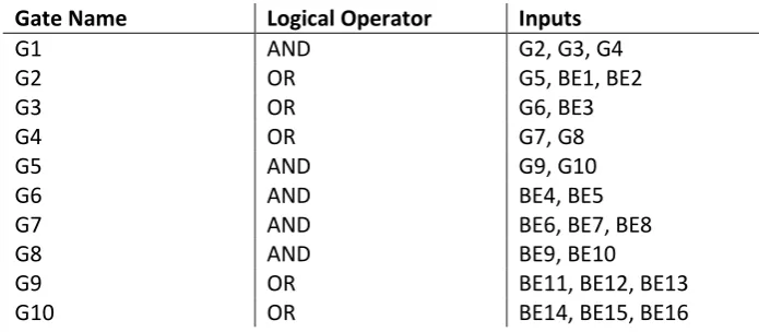
Table A.1 - Fault tree description for system 1.
Gate Name Logical Operator Inputs
G1 AND G2, G3, G4
G2 OR G5, BE1, BE2
G3 OR G6, BE3
G4 OR G7, G8
G5 AND G9, G10
G6 AND BE4, BE5
G7 AND BE6, BE7, BE8
G8 AND BE9, BE10
G9 OR BE11, BE12, BE13
G10 OR BE14, BE15, BE16
Table A.2 – Components and component types for system 1.
Component Component Type
BE1 1
BE2 2
BE3 1
BE4 1
BE5 3
BE6 2
BE7 2
BE8 1
BE9 1
BE10 3
BE11 1
BE12 2
BE13 2
BE14 1
BE15 1
20
[image:20.595.70.527.70.761.2]Appendix B – Signatures for system 1 and the European 3 system.
Table B.1a – Part 1 of survival signature for system 1.
𝒍𝟏 𝒍𝟐 𝒍𝟑 Survival
signature value 𝚽𝒍𝟏,𝒍𝟐,𝒍𝟑
𝒍𝟏 𝒍𝟐 𝒍𝟑 Survival
signature value 𝚽𝒍𝟏,𝒍𝟐,𝒍𝟑
9 5 2 1.0000 7 2 2 0.9972
9 5 1 1.0000 7 2 1 0.9875
9 5 0 1.0000 7 2 0 0.9611
9 4 2 1.0000 7 1 2 0.9889
9 4 1 1.0000 7 1 1 0.9722
9 4 0 1.0000 7 1 0 0.9333
9 3 2 1.0000 7 0 2 0.9722
9 3 1 1.0000 7 0 1 0.9444
9 3 0 1.0000 7 0 0 0.8889
9 2 2 1.0000 6 5 2 1.0000
9 2 1 1.0000 6 5 1 0.9940
9 2 0 1.0000 6 5 0 0.9762
9 1 2 1.0000 6 4 2 1.0000
9 1 1 1.0000 6 4 1 0.9798
9 1 0 1.0000 6 4 0 0.9214
9 0 2 1.0000 6 3 2 0.9988
9 0 1 1.0000 6 3 1 0.9690
9 0 0 1.0000 6 3 0 0.8857
8 5 2 1.0000 6 2 2 0.9821
8 5 1 1.0000 6 2 1 0.9399
8 5 0 1.0000 6 2 0 0.8369
8 4 2 1.0000 6 1 2 0.9571
8 4 1 1.0000 6 1 1 0.9024
8 4 0 1.0000 6 1 0 0.7857
8 3 2 1.0000 6 0 2 0.9167
8 3 1 1.0000 6 0 1 0.8452
8 3 0 1.0000 6 0 0 0.7143
8 2 2 1.0000 5 5 2 1.0000
8 2 1 1.0000 5 5 1 0.9643
8 2 0 1.0000 5 5 0 0.8651
8 1 2 1.0000 5 4 2 1.0000
8 1 1 1.0000 5 4 1 0.9405
8 1 0 1.0000 5 4 0 0.7873
8 0 2 1.0000 5 3 2 0.9929
8 0 1 1.0000 5 3 1 0.9175
8 0 0 1.0000 5 3 0 0.7333
7 5 2 1.0000 5 2 2 0.9548
7 5 1 1.0000 5 2 1 0.8647
7 5 0 1.0000 5 2 0 0.6690
7 4 2 1.0000 5 1 2 0.9048
7 4 1 0.9972 5 1 1 0.8016
7 4 0 0.9889 5 1 0 0.6032
7 3 2 1.0000 5 0 2 0.8333
7 3 1 0.9944 5 0 1 0.7143
21
Table B.1b – Part 2 of survival signature for system 1.
𝒍𝟏 𝒍𝟐 𝒍𝟑 Survival
signature value (𝚽𝒍𝟏,𝒍𝟐,𝒍𝟑)
𝒍𝟏 𝒍𝟐 𝒍𝟑 Survival
signature value (𝚽𝒍𝟏,𝒍𝟐,𝒍𝟑)
4 5 2 1.0000 2 2 2 0.8250
4 5 1 0.9048 2 2 1 0.5708
4 5 0 0.6825 2 2 0 0.1917
4 4 2 1.0000 2 1 2 0.6500
4 4 1 0.8802 2 1 1 0.4333
4 4 0 0.6143 2 1 0 0.1333
4 3 2 0.9810 2 0 2 0.4167
4 3 1 0.8452 2 0 1 0.2500
4 3 0 0.5595 2 0 0 0.0556
4 2 2 0.9183 1 5 2 1.0000
4 2 1 0.7742 1 5 1 0.6111
4 2 0 0.4952 1 5 0 0.1111
4 1 2 0.8349 1 4 2 1.0000
4 1 1 0.6841 1 4 1 0.6111
4 1 0 0.4222 1 4 0 0.1111
4 0 2 0.7222 1 3 2 0.9222
4 0 1 0.5635 1 3 1 0.5611
4 0 0 0.3254 1 3 0 0.1000
3 5 2 1.0000 1 2 2 0.7667
3 5 1 0.8214 1 2 1 0.4611
3 5 0 0.4762 1 2 0 0.0778
3 4 2 1.0000 1 1 2 0.5333
3 4 1 0.8036 1 1 1 0.3111
3 4 0 0.4333 1 1 0 0.0444
3 3 2 0.9643 1 0 2 0.2222
3 3 1 0.7601 1 0 1 0.1111
3 3 0 0.3893 1 0 0 0.0000
3 2 2 0.8750 0 5 2 1.0000
3 2 1 0.6756 0 5 1 0.5000
3 2 0 0.3333 0 5 0 0.0000
3 1 2 0.7500 0 4 2 1.0000
3 1 1 0.5595 0 4 1 0.5000
3 1 0 0.2619 0 4 0 0.0000
3 0 2 0.5833 0 3 2 0.9000
3 0 1 0.4048 0 3 1 0.4500
3 0 0 0.1667 0 3 0 0.0000
2 5 2 1.0000 0 2 2 0.7000
2 5 1 0.7222 0 2 1 0.3500
2 5 0 0.2778 0 2 0 0.0000
2 4 2 1.0000 0 1 2 0.4000
2 4 1 0.7139 0 1 1 0.2000
2 4 0 0.2611 0 1 0 0.0000
2 3 2 0.9444 0 0 2 0.0000
2 3 1 0.6653 0 0 1 0.0000
22
Table B.2 – System signature for system European 3.
Number of failed components
(j)
System signature value (𝒒𝒋)
Number of failed components
(j)
System signature value (𝒒𝒋)
Number of failed components
(j)
System signature value (𝒒𝒋)
1 0.00E+00 28 1.36E-09 55 9.41E-03
2 0.00E+00 29 3.55E-09 56 1.24E-02
3 0.00E+00 30 8.81E-09 57 1.60E-02
4 0.00E+00 31 2.10E-08 58 2.02E-02
5 0.00E+00 32 4.80E-08 59 2.49E-02
6 0.00E+00 33 1.06E-07 60 3.01E-02
7 0.00E+00 34 2.27E-07 61 3.56E-02
8 0.00E+00 35 4.72E-07 62 4.12E-02
9 0.00E+00 36 9.54E-07 63 4.67E-02
10 0.00E+00 37 1.88E-06 64 5.18E-02
11 0.00E+00 38 3.60E-06 65 5.63E-02
12 0.00E+00 39 6.76E-06 66 5.99E-02
13 0.00E+00 40 1.24E-05 67 6.24E-02
14 0.00E+00 41 2.22E-05 68 6.37E-02
15 0.00E+00 42 3.91E-05 69 6.37E-02
16 0.00E+00 43 6.72E-05 70 6.22E-02
17 0.00E+00 44 1.13E-04 71 5.95E-02
18 5.55E-16 45 1.88E-04 72 5.55E-02
19 5.66E-15 46 3.04E-04 73 5.04E-02
20 4.09E-14 47 4.83E-04 74 4.43E-02
21 2.28E-13 48 7.53E-04 75 3.74E-02
22 1.08E-12 49 1.15E-03 76 3.00E-02
23 4.44E-12 50 1.72E-03 77 2.23E-02
24 1.64E-11 51 2.52E-03 78 1.45E-02
25 5.51E-11 52 3.62E-03 79 6.96E-03
26 1.71E-10 53 5.08E-03 80 0.00E+00