A hysteretic multiscale formulation for validating computational models of heterogeneous structures

Abstract

A framework for the development of accurate yet computationally efficient numerical models is proposed in this work, within the context of computational model validation. The accelerated computation achieved herein relies on the implementation of a recently derived multiscale finite element formulation, able to alternate between scales of different complexity. In such a scheme, the micro-scale is modeled using a hysteretic finite elements formulation. In the micro-level, nonlinearity is captured via a set of additional hysteretic degrees of freedom compactly described by an appropriate hysteric law, which gravely simplifies the dynamic analysis task. The computational efficiency of the scheme is rooted in the interaction between the micro- and a macro-mesh level, defined through suitable interpolation fields that map the finer mesh displacement field to the coarser mesh displacement field. Furthermore, damage related phenomena that are manifested at the micro-level are accounted for, using a set of additional evolution equations corresponding to the stiffness degradation and strength deterioration of the underlying material. The developed modeling approach is utilized for the purpose of model validation; firstly, in the context of reliability analysis; and secondly, within an inverse problem formulation where the identification of constitutive parameters via availability of acceleration response data is sought.

Keywords

A Hysteretic Multiscale formulation for

Validating Computational Models of

Heterogeneous Structures

©The Author(s) 2010 Reprints and permission:

sagepub.co.uk/journalsPermissions.nav DOI:10.1177/1081286510367554 http://mms.sagepub.com

Savvas P. Triantafyllou

_{and Eleni N. Chatzi}

1

_{Department of Civil Engineering, The University of Nottingham, UK}

2

_{Institute of Structural Engineering, Department of Civil, Environmental and Geomatic Engineering,}

ETH Zürich, Switzerland

1. Introduction

Engineering simulation is an essential feature accompanying the design, manufacturing and operational life of every engi-neered structure. However, and despite the refinement and complexity that such simulations might entail, these are not routinely validated, largely due to the computational cost associated with the multiplicity of parallel runs involved. This inadequacy comes in direct disagreement with the recent advances both in monitoring methodologies as well as in compu-tation potential. The former has provided engineers with low-cost means of assessing structural performance, both during the construction phase as well as during the operational of a structural system. Significant feedback is therefore collected from the system at hand, which may then be utilized for selecting, updating and/or validating candidate computational models.

A significant source of complexity within computation stems from the potential multi-phase nature of materials com-prising the system to be analyzed. Multiphase materials, also known as composites, fit the profile of emerging material solutions calling for enhanced computation. In most industrial cases, the main volume of a composite consists of a single material (e.g. the matrix) that acts as a basis where a number of reinforcing materials are added. The distribution of the reinforcement within the matrix can be either fully prescribed, as in the case of layered composites, or random, as in the case of fibre reinforced matrices. This process of mechanically combining constituent materials baring different properties results into a highly heterogeneous structure. Due to the advanced material properties of the resulting medium,composites are widely used in numerous applications. Research efforts currently focus on developing and manufacturing composites with enhanced mechanical properties (e.g. high stiffness to weight ratios, high damping, negative Poisson’s ratio and high toughness1_{) and reduced implementation and maintenance costs}2–4_{. Recent advances in fields such as bioengineering,}

nano-mechanics and electronics also stress the need for designing new composites with optimal material properties5,6. Nonetheless, prior to proceeding with design refinement appropriate methodologies need to be developed, for validating the numerical models simulating these solutions .

Model validation7_{may be carried out via two distinct routes, which however can be intertwined. The first path is through}

numerical validation,also referred to as numerical verification8_{, in the sense that most practical models to be employed}

are usually inferred by adopting a number of simplifying assumptionsin an effort to reduce the required computational toll. A first step toward validating such models is through comparison with either benchmark analytical solutions, or when this is not possible, with more refined/higher dimensional numerical solutions, which may be considered as a closer approximation of the true system. If the reduced order model successfully reproduces the desired response with a sufficient level of accuracy, lying below some acceptable threshold, it may then be adopted for the forward simulation of the system at hand. The second route, which is invaluable within the context of standardization of the validation approach, is through experimental validation as noted in9–11_{. This route relies on the use of actual structural feedback, i.e., through experimental}

or field measurements of structural response under static or dynamic loads.

Indeed, when it comes to composites, significant effort has been allocated in developing simulation models that comply with experimentally measured response, via an inverse problem formulation12. In past years, several methods have been introduced along the lines of the so-called mixed numerical-experimental techniques for the successful modeling of polymer based materials and composite reinforcing textiles13,14_{. The anisotropic and heterogeneous nature of these materials turns the}

direct determination of stiffness parameters into an arduous task. Conventional methods are based on direct measurements of strain fields15_{, presenting several drawbacks such as boundary effects, sample size dependencies and difficulties in}

obtaining homogeneous stress/strain fields16. As an alternative, indirect methods based on modal test data have become more popular in recent years. These are based on measurements of structural response and the comparison between the experimentally identified eigen-frequencies of a structure and those obtained through a numerical analysis employing a finite element model17–19_{. This inverse problem formulation can lead to an estimate of the macroscopic material parameters}

of the composite materials, which are generally impossible to standardize in tables or databases as they are dependent on diverse factors such as the geometrical arrangement of the laminates, constituent materials used, manufacturing process etc. Independent of whether a direct or indirect method is employed, a forward model of the structure is required for deriving those parameters that are deemed as uncertain, most commonly those pertaining to the effective moduli.

However, the sensitivity of the identified parameters to the size of the testing specimen20,21_{imposes a strong constraint}

on the required size of the underlying finite element model leading to computationally intensive problems22_{. To reduce}

the computational cost, multiscale simulation approaches have been introduced23–25. Two main variants of computational multiscale analysis methods can be identified,namely the multiscale homogenization methods26 _{and multiscale finite}

element methods (MsFEMs)27.

Homogenization methods are based on averaging strain and energy conjugate stress measures over a predefined space domain, defined as a Representative Volume Element (RVE)28_{. Although homogenization methods are based on a strong}

and robust mathematical background, they rely on the assumption of scale separation and local periodicity of the underlying micro-structure. Many structures however usually fail to adhere to these assumptions, due to the non-periodic nature of the imposed boundary and loading conditions that lead to non-periodic stress and strain fields as well as the non-deterministic distribution of heterogeneities within them. To overcome these deficiencies the multiscale finite element method has been introduced. In this, the macro-scale of the structure is discretized into a set of coarse elements. These coarse elements are further discretized into sets of nested meshes. Next, a set of interpolation functions is evaluated, mapping micro- to macro-displacement components . The MsFEM method has been extensively used in flow simulation analysis27,29_{. Recently the}

Enhanced Multiscale Finite Element method (EMsFEM) has been formulated to address the linear and nonlinear response of heterogeneous materials30_{under static loads.}

observed at the macro-scale. Within this framework, the hysteretic multiscale finite element method (HMsFEM) has been introduced in recent work of the authors31_{, which forms a tool for significantly reducing the computational cost of nonlinear}

dynamic analysis of complex structures.According to this approach, inelasticity is accounted for at the fine mesh level using the hysteretic formulation of finite elements32_{. The latter is based on the definition of a set of additional degrees of}

freedom regulating the evolution of the plastic component of elemental deformation. Since inelasticity is treated as a degree of freedom, the element stiffness matrix remains unchanged throughout the whole analysis. As a result, the evaluation of the micro-basis functions is also performed once. The evolution of the additional degrees of freedom is constrained by a set of additional equations that account for the constitutive behavior of the underlying material. A smooth plasticity model is employed to describe the evolution of plastic strains at the micro-scale. The computational merits of the hysteretic multiscale finite element method have been discussed within a reliability framework in33,34. Herein, damage accumulation is also accounted for, by introducing an additional set of internal variablesaccounting for the gradual degradationof the material’s unloading stiffness as well as the deterioration of the material’s yield limit.

In the work presented herein, the previously introduced HMsFEM approach serves as the tool for model validation, under a stochastic setting, in twotypesof problems. The first application pertains to a reliability analysis problem, where structural response is quantified in a probabilistic sense using a Monte Carlo approach.The proposed modeling methodology is in this case verified against a refined, albeit computationally intensive, FE model. Composites are intrinsically multiscale materials where uncertainties stemming at the smaller, constituent, scale greatly affects the behaviour of the larger, structural, scale35,36_{. Thus, the stochastic analysis of such materials under conditions of extreme loading is of paramount importance in}

order to quantify the probability of failure of the corresponding structure. Since the reliability analysis of structures per-se is a computationally intense procedure, it is pointed out that multiscale models37_{should be preferred over standard stochastic}

FEM procedures38_{, in an effortto reduce the complexity of the implemented computational model without adverse effects}

on the desired accuracy. The second application pertains to an inverse problem formulation, where the identification of the uncertain material parameters of a composite structure, namely, the structural stiffness and strength at the level of the constituents, is sought, based on recorded acceleration response from limited structural nodes.

The paper is structured as follows. In the next section, the Enhanced Multiscale Finite Element Method (EMs-FEM) is overviewed. Next, the constitutive model implemented at the micro-scale is presented in the section titled Micro-scale Constitutive modeling. The model presented herein is an extension of the smooth model presented by

the authors in32 _{accounting for damage phenomena relating to cyclic loads, i.e. the degradation of the material}

stiff-ness and the deterioration of the corresponding yield strength. This material model is then implemented within the enhanced multiscale finite element scheme and the corresponding derivations are presented in the section entitled The hysteretic multiscale finite element method with damage. Although straightforward, the use of the additional damage

operators is not trivial as it affects both the evolution equation of the plastic deformation tensor as well as the out-of-balance forces of the micro-elements. The section titledComputational Model Validationbriefly discusses the computational tools that are here adopted for the purpose of model validation, from both a numerical and experimental standpoint. Finally, illustrative applications are presented in theExemplary Implementationssection validating the proposed derivations and demonstrating the computational advantages of the developed framework, firstly under the scope of reliability assessment and, secondly, within the context of an inverse problem formulation.

2. The enhanced multiscale finite element method

2.1. Overview

EMsFEM is based on the definition of a set of nested finite element meshes as explained in30_{. The interaction between}

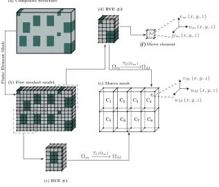
structure is presented for brevity. The composite comprises a matrix and a set of reinforcing cells. Based on the distribution of the cells within the matrix, a fine discretization scheme is defined, consisting of 384 linear hex-elements and 663 nodes that correspond to 1989 degrees of freedom.

Depending on the micro-structure’s periodicity, patterns of heterogeneity can be recognized and sets of micro-elements can be grouped into clusters,which will herein be denoted as Representative Volume Elements or RVEs. The convex-hull of each cluster defines a coarse-element (or macro-element) that surrounds the fine-meshed RVE substructure. In Fig.1 two distinct patterns are identified and the corresponding RVEs are presented in Fig. 1(c) and 1(d). The set of coarse elements results in the definition of the coarse mesh presented in Fig.1(e). This mesh consists of 8 coarse elements and 30 macro-nodes that correspond to 90 macro-degrees of freedom (dofs).

According to EMsFEM, instead of performing a finite element analysis on the fine mesh (Fig.1(a)),a numerical interpolation schemeT_{iis evaluated for each RVE(i).The latter maps the displacementsumof the corresponding}

micro-nodes, defined within the micro-domainΩm, onto the macro-displacementuMfield, defined in the macro-domainΩM.

With respect to Fig.1(f), the fine mesh the displacement of a micro pointpis described by relation (1) below

u_m={umvmwm}T|(x,y,z) (1)

The continuous micro-displacement field introduced in relation (1) can be interpolated at the micro-nodal points using a standard displacement based FE interpolation scheme as in39

u_m= [N]_mdim (2)

where

di

m=

n

um(1) vm(1) · · · vm(8)

oT

| {z }

1x24

(3)

is the nodal displacements vector of theithmicro-element,and[N]_mis the displacement based interpolation matrix of the hex-element.

Since the structure defined in Fig.1(e) is a discrete macro-representation of the physical model consisting of the RVEs, the macro-displacement component within each RVEdi

M can be defined accordingly as the discrete set such that di

M =

n

uM(1) vM(1) · · · vm(8)

oT

| {z }

1x24

(4)

where(i)stands for theithmacro-node of the coarse mesh.

The subscriptmis used throughout this manuscript to denote a micro-measure, while the capitalM is used to denote a macro-measure of the indexed quantity. The enhanced multiscale Finite Element method is based on the numerical derivation of a relation between the discrete micro-displacement field introduced in equation (3) and the coarse element discrete displacement field introduced in relation (4).

2.2. Micro to Macro displacement interpolation scheme

(f )

p p

Fig. 1. The MsFE modeling scheme

of the following interpolation scheme where the micro-displacement components are evaluated with respect to the macro-displacement components as:

um(j)= nM acro

P

i=1

NijxxuMi+

nM acro P

i=1

NijxyvMi

+n

M acro P

i=1

NijxzwMi

vm(j)= nM acro

P

i=1

NijxyuMi+

nM acro P

i=1

NijyyvMi

+n

M acro P

i=1

NijyzwMi

wm(j)= nM acro

P

i=1

NijxzuMi+

nM acro P

i=1

NijyzvMi

+n

M acro P

i=1

NijzzwMi

(5)

whereum(j),vm(j),wm(j) are the displacement components of thejth micro-node,j = 1...nmicro wherenmicro the

number of micro nodes within the coarse element. Furthermore,nM acro is the number of macro-nodes of the coarse element anduMi,vMi,wMiare the displacement components of the macro-nodes of theithcoarse-element.

The quantitiesNijxx,Nijxy,Nijyy,Nijzz,Nijxz.Nijyzare the micro-basis interpolation functions. These interpolate the displacement components of thejthmicro-node to the macro-displacement components of the correspondingithcoarse element.

Equation (5) is derived in matrix form as:

{d}_m(i)= [N]_m(i){d}_M (6)

displacements. Denoting{d}_mthe(3nmicro×1)vector of the micro-mesh nodal displacements, the following relation is established:

{d}_m= [N]_m{d}_M (7)

Matrix[N]_min equation (7) is a315×24matrix containing the components of the micro-basis shape functions evaluated at the nodal points(xj, yj, zj)of the micro-mesh. Each column of matrix[N]_mcorresponds to a deformed configuration of the RVE where the corresponding macro-degree of freedom is equal to unity and all the rest macro-degrees of freedom are equal to zero.

The micro-basis functions are derived as the solution of the boundary value problem defined in equation (8) below

[K]_RVE{d}_m={/0}

{d}_S =d¯

(8)

where[K]_{RV E} denotes the stiffness matrix corresponding to the coarse element,{d}_S is the vector containing the nodal degrees of freedom lying along the boundarySof the coarse element andd¯ is a vector of prescribed displacements. Vector{/0}is the zero vector. The coarse element stiffness matrix is assembled via the standard finite element method39_.

The application of the prescribed boundary conditions and the solution of the boundary value problem of equation (8) is performed herein using the Penalty method40.

The accuracy of the method depends on the proper choice of the assumed boundary conditions for the evaluation of the micro-basis functions and is naturally dictated by the kinematics of the problem at hand, as well as the size of the coarse element. Different methodologies exist including the linear, periodic and oscillatory boundary conditions with oversampling. Further details can be found in30,41_.

3. Micro-scale Constitutive modeling

In this Section, the constitutive model governing the material behaviour at the micro-scale is presented. The model presented herein is derived on the basis of the theory of classical plasticity, also introducing a set of additional material parameters accounting for the smoothness of the transition from elastic to plastic loading and from plastic loading to elastic unloading. Furthermore, two damage operators are introduced corresponding to the degradation of the unloading stiffness and the deterioration of the material yield strength due to cyclic loading induced damage.

3.1. Smooth hysteretic modeling

The hysteretic formulation of finite elements32 is implemented herein to account for the nonlinear dynamic behavior of materials at the micro-scale. In this, a mixed interpolation scheme is considered for both the displacement and the plastic component of the strain tensor. An evolution relation is extracted from the latter based on the additive decomposition of the total strain tensor into a reversible elastic and an irreversible inelastic component42_:

{ε˙}_m(i)=ε˙el

m(i)+

˙ εpl

m(i) (9)

where{ε}_m(i)is the total strain tensor,εel

m(i)is the tensor of the elastic, reversible, strain and

εpl

m(i)is the plastic

elastic component of the strain tensorεel

m(i)is directly related to the current stress{σ}m(i)through the Hooke’s law

{σ˙}_m(i)= [D]_m(i)ε˙el

m(i) (10)

where[D]_m(i)is the elastic constitutive matrix43_{. Additionally, an evolution law is considered for the plastic component}

of deformation, generically defined as:

˙

εpl _m(i)=F_εel m(i),

˙

εel _m(i),{σ}_m(i)

(11) whereF _{is an hysteretic operator}44,45_.

In this work, the hysteretic operator is defined on the grounds of a multi-axial smooth plasticity model32_{based on the}

assumptions of rate-independent associative plasticity46. Within such a framework, the evolution of the plastic strain tensor is defined as

˙ εpl

m(i)=H1H2[R]{ε˙}m(i) (12)

whereH1andH2are smoothened Heaviside functions defined by the following relations, namely:

H1=

Φ{σ}_m(i),{η}_m(i)

Φ0

N

, N ≥2 (13)

and

H2=β+γsgn

˙Φ (14)

In equation (13)Φ = Φ{σ}_m(i),{η}_m(i)denotes the yield criterion,Φ0the yield limit,Ndetermines the rate at which

the yield criterion reaches its peak value whileβ andγare material parameters that define the stiffness at the point of unloading. The time derivative of the yield function in equation (14) is derived from the following expression

˙

Φ = ∂Φ

∂{σ}m(i) ˙

{σ}_m(i)+

∂Φ ∂{η}m(i)

˙

{η}_m(i) (15)

Matrix[R]in equation (12) is a strain interaction matrix defined as

[R] ={α}Q{α}T[D] (16)

where

Q=− {b}TG{η}_m(i),Φ+ (α)T[D]{α}−1 (17)

and column vectors{α}and{b}are defined as

{α}=∂Φ.∂{σ}

and

{b}=∂Φ.∂{η}

respectively, whileG{η}_m(i),Φis defined herein as the hardening function.The associated kinematic hardening rule assumes the following form

whereλ˙

˙ λ=ε˙pl

m(i) ∂Φ ∂{σ}_m(i)

is the plastic multiplier defined in the work of Lubliner46.

Since the yield function in relation (13) depends on the back-stress a second equation is also introduced for the evolution of that stress with respect to the strain:

{η˙}=H1H2G

{η}_m(i),Φ

h ˜

Ri{ε˙}_m(i) (19)

where

h ˜

Riis the defines the hardening interaction as

h ˜

Ri=Q{α}T[D] (20)

Equations (9) and (10) imply that during unloading the material stiffness is constant and equal to the elastic one.

3.2. Cyclic loading induced damage

The model presented in the section titledSmooth hysteretic modelingis enhanced herein to account for damage effects. This is accomplished by introducing two additional internal parameters within the hysteretic finite element scheme accounting for the degradation of the elastic material stiffness and the deterioration of the yield limit. These parameters are accompanied by a set of corresponding evolution equations that depend on the hysteretic energy accumulated over time. The relations are based on the derivations introduced in47_{,where a proof is also derived for the thermodynamic admissibility of the}

corresponding material model.

The elastic stiffness degradation parameter is introduced at the stress-strain relation (10):

{σ˙}_m(i)=vη[D]_m(i)ε˙el

m(i) (21)

wherevηis a degradation parameter that is equal to unity as long as the material has not yielded and increases with plastic deformation. The following generic expression is thus defined:

˙

vη=K_{η Ehm(i) (22)}

whereEhm(i)is the hysteretic energy of theithmicro-element.

Solving equation (9) forε˙el _{and substituting into equation (21) the following relation is finally derived:}

{σ˙}_m(i)=vη[D]_m(i){ε˙}_m(i)−ε˙pl

m(i)

(23) where the total stress tensor comprises a function of the total and plastic strain tensors and the degradation parameter. For the purpose of this work, a constant rate stiffness degradation rule is considered and thus relation (22) is expressed as

. vη =cη cη|_Eh=0= 1.0

)

⇒vη = 1.0 +cηEhm(i) (24)

i ci hi

1 280e6 kPa 850

2 100e3 kPa 500

3 50e3 kPa 8

4 1e3 kPa 5

5 0.1 kPa 1

Table 1: Chaboche model parameters

Yield deterioration is accounted for by introducing parametervsinto the yield related smooth Heaviside function1

defined in relation (13)

H1=vs

Φ{σ}_m(i),{η}_m(i)s Φ0

N

, N ≥2 (25)

where in generalvsis a function of the hysteretic energy accumulated within the element

˙

vs=K_{v Ehm(i) (26)}

A constant rate evolution law is also considered in this work, thus the variation of the strength deterioration parametervs

is defined as

. vs=cs vs|_Eh=0= 1.0

)

⇒vs= 1.0 +csEhm(i) (27)

wherecsis a user defined material parameter.

3.3. Example

To better demonstrate the influence of the hysteretic parameters implemented in the model,the case of steel bar under uniaxial tension is considered. The elastic modulus of the bar isEs= 210GP aand the initial yield stresssy= 235M P a. The following parameters are considered for the smooth model, namelyn = 2andβ = γ = 0.5. A von-Mises yield criterion is considered. Two cases of hardening are examined. In the first, linear kinematic hardening is considered with the hardening modulusH= 4GP a. The hardening functionGin relation (18) is therefore defined as

G= 4 ∂Φ

∂{σ}

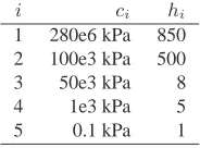
In the second case, a Chaboche additive nonlinear kinematic hardening rule is considered48_{, where hardening function is}

defined as:

G=∂Φ

∂σ 5 X

1 2 3hi−

r 2 3ciη

!

(28)

The model parameters for the Chaboche kinematic hardening are presented in Table1. The bar is subjected to sinusoidal imposed strain according to the following equation

ε= 0.01 π sin(πt)

−0.4 −0.2 0 0.2 0.4 −400

−300 −200 −100 0 100 200 300 400

Normal Strain εxx [%]

Normal Stress [Mpa]

Chaboche Linear

Fig. 2. Stress-strain diagrams - no degradations

Next, stiffness degradation and strength deterioration are taken into account by settingcη = 0.0000002andcs = 0.000001respectively. The corresponding results are presented in Fig.3.

−0.4 −0.2 0 0.2 0.4 −400

−300 −200 −100 0 100 200 300 400

Normal Strain εxx [%]

Normal Stress [Mpa]

Chaboche Linear

Fig. 3. Stress-strain diagrams - stiffness degradation/ strength deterioration

4. The hysteretic multiscale finite element method with damage

In this Section the derivation of the governing equations of the Hysteretic Multiscale Finite Element method is presented. Based on a variational formulation introduced in the micro-scale and using the constitutive model introduced in the previous Section, the micro-element governing equations are established. Next, using the micro to macro numerical mapping procedure, these governing equations are mapped to the macro-scale where solution is performed.

4.1. Micro-scale discrete formulation

The hysteretic multiscale finite element method is naturally derived from the rate form of the Principle of Virtual Work49 presented in equation (29)

Z

Ve

{ε}T_m(i){σ˙}_m(i)dVe={d}T_m(i)nf˙o

whereVeis the volume of the discrete element,{d}_m(i)is the vector of nodal displacements andnf˙o

m(i)is the vector of

energy conjugate nodal forces. Substituting equation (9) into the variational principle (29) the following relation is derived:

Z

Ve

{ε}T_m(i)vη[D]_m(i){ε˙}_m(i)−ε˙pl m(i)

dVe=

={d}T_m(i)nf˙o m(i)

(30)

Following algebraic manipulations and by considering thatvη ≥1.0, the following expression is derived:

I_el−I_pl= 1 vη {d}

T m(i)

n ˙ fo

m(i) (31)

where

I_el= Z

Ve

{ε}T_m(i)[D]_m(i){ε˙}_m(i)dVe (32)

and

I_pl= Z

Ve

{ε}T_m(i)[D]_m(i)ε˙pl

m(i)dVe (33)

In this work, the isoparametric interpolation scheme is considered for the displacement field

{d}_m(i)= [N]{u}_m(i) (34)

where [N]_m(i) is the shape function matrix. The corresponding strain-displacement relation is derived through compatibility39_{and assumes the following form}

{ε}_m(i)= [B]{u}_m(i) (35)

where[B]is the strain-interpolation matrix.

An additional interpolation scheme is introduced for the plastic deformation

˙ εpl

m(i)= [N]e

˙ εpl

cq _m(i) (36)

whereεpl

cq _m(i) is the vector of stains measured at properly defined collocation points and[N]e is the corresponding

interpolation matrix.

Substituting relations (35) and (36) onto equation (30), the following relation is derived

kel

m(i) n

˙ do

m(i)−

kh m(i)

˙ εpl

cq _m(i)= 1 vη

n ˙ fo

m(i) (37)

where

kel

m(i)= Z

Ve

[B]T[D]_m(i)[B]dVe (38)

is the element elastic stiffness matrix whilekh m(i)

kh

m(i)= Z

Ve

is the hysteretic matrix. Bothkel

m(i)and

kh

m(i)are constant. Nonlinearity is introduced at the additional collocation

points where the evolution of plastic deformations is measured. This evolution can be generically defined in the form of equation (11).

In the case of the composite structure presented in Figure1, the element elastic stiffness matrixkel

m(i)coincides with

the24×24stiffness matrix of the 8-node brick element50. The dimension of the hysteretic matrixkh

m(i)depends also

on the number of collocation points. Considering the case where full integration is performed and the collocation points are chosen to coincide with the Gauss point would result in a24×48hysteretic matrix.

4.2. Micro to Macro transformation

Considering zero initial conditions, without loss of generality, the rates in equation (38) can be dropped resulting in:

kel

m(i){d}m(i)−

kh m(i)

εpl

cq (i)= 1

vη{f}m(i) (40)

Substituting equation (6) into equation (40) and pre-multiplying with[N]T_m(i)the following is attained:

kelM_m(i){d}_M −khM_m(i)εplcq _(i)= 1 vη {f}

M

m(i) (41)

where

kelM_m(i)= [N]T_m(i)kel_m(i)[N]_m(i) (42) is the elastic stiffness matrix of theith micro-element mapped onto the macro-element dofs whilekhM

m(i)is the

micro-element hysteretic matrix of theithevaluated as:

khM_m(i)= [N]T_m(i)kh_m(i) (43)

Finally,{f}M_m(i)in equation (41) is the equivalent nodal force vector of the micro-element mapped onto the coarse element nodes (macro-nodes).

{f}M_m(i)= 1

vη [N] T

m(i){f}m(i) (44)

Equation (41) maps the micro-element equilibrium equation established in equation (40) from the micro-scale to the macro-scale. The micro-displacement components{u}_m(i) are mapped onto their macro-counterparts through relation (6). Consequently, the elastic micro-constitutive behavior is communicated across scales through the EMsFEM numerical mapping. Inelasticity is accounted for in the micro-scale throughthe evolution of themicro-plastic deformation quantities

εpl

cq _(i)and mapped onto the macro-scale through the transformed hysteretic matrix

khM m(i).

Relations (42) and (43) are then assembled at the macro-scale to derive the coarse element equilibirum equation which assumes the following form

[K]M_CR(j){d}_M ={f}_M − {fh}_M (45)

where[K]M_CR(j)is the equivalent stiffness matrix of the coarse element derived as

[K]M_CR(j)= i X

1

kelM

while{f}_M is the corresponding nodal force vector assembled from the contributions of the mapped micro-nodal force components defined in relation (44) and{fh}_M is the force vector of the plastic components evaluated as

{fh}_M =

mel X

i=1

khM m(i)

εpl

cq m(i) (47)

Equation (45) is derived upon enforcing the energy equivalence principle between the deformation energy of the coarse element and the deformation energy of the corresponding micro-mesh31. This is not an assumption of the method, but a relation that is directly derived from the fact that the coarse element is a mathematical entity whose mechanical properties are only defined at the micro-scale. Having defined the equivalent coarse element elastic stiffness and hysteretic matrices, the direct stiffness method is implemented to finally derive the governing equations at the structural level. Defining as

ndofM the number of the free macro-degrees of freedom, the equations of motion of the structure assume the following form

[M]nU¨o

M + [C] n

˙ Uo

M + [K]{U}M ={P}M

(48) The coarse mesh(ndofM ×1)nodal load vector{P}_M in relation (48) is derived as

{P}_M ={F}_M +{Fh}_M (49)

where{F}_M is the(ndofM×1)vector of externally applied loads and{Fh}_M is the(ndofM ×1)hysteretic load vector assembled for the whole structure. Matrices[M],[C]and[K]are the(ndofM ×ndofM)mass, viscous damping and elastic stiffness matrix of the structure evaluated at the coarse mesh.

Equations (48) are complemented by the micro-plastic strain evolution equations:

n ˙ Epl

cq o

m= [H]{εcq˙ }m

(50) where the vector

n ˙ Ecqpl

o

m=

n ˙ εpl

cq _m(1) · · ·

˙ εpl

cq _m(mel) oT

(51) contains the plastic strains evaluated at the collocation points of each micro-element and

n ˙ Ecqo

m=

n

{εcq˙ }_m(1) · · · ε˙cq _m(mel)

oT

(52)

Matrix[H]in relation (50) is a block diagonal matrix:

[H] = 

  

A_{(1) [0]}

[0] . .. A_(m

el) 

 

 (53)

whereA_{(1)=H1m(1)H2m(1)[R]}

m(1)andA(mel)=H1m(mel)H2m(mel)[R]_m(_mel)

derive the corresponding strain increments at themicro-scale. The computational aspects of the methodology presented herein are described in detail in31_.

5. Computational Model Validation

As aforementioned, validation of computational models may be discussed in relation to two main directions, namely, the numerical verification and the experimental validation approach.Within the context of computational model validation, we herein exemplify both instances (a) via cross-comparison of the proposed HMsFEM approach to a reference fine-mesh model; and (b) via validating the proposed model in an inverse formulation employing (simulated) structural testing data.

5.1. Numerical Verification via Monte Carlo Simulation

Within the scope of what is discussed herein, it is evident that as the complexity of the system increases, the formulation of exact models becomes a challenging task. In validating the efficacy of the assumptions and simplifications that need be adopted, the Monte Carlo method comprises a useful tool for reliability prediction. Unlike many other mathematical models, system complexity is not a hindrance for this approach, which can handle dynamic systems of an imprecise nature. This is particularly useful in the case of a reliability analysis, which entails processes of a probabilistic nature. These processes usually analyze the effects of the combination of two or more input random variables onto the probability distribution of certain output random variables. In approaching such a problem one could resort to either analytical methods or to Monte-Carlo simulation. In the analytical approach, the probability distributions associated with the output are derived via analytical formulations, which involvethe probability distribution functions (PDFs) associated with the input. Since such a straightforward formulation is cumbersome depending on the problem at hand, Monte Carlo simulation offers a valuable alternative. Following this approach, a sample space of the input parameter is generated via use of a random number and knowledge of its PDF. By repeating this process for a large number of input samples, a picture of the distribution of the output random variable is attained, which ultimately leads into statistical estimates of parameters of interest, e.g. mean and standard deviation of failure probability, or maximum inter-storey drift ratios. Through a variety of implementations, the Monte Carlo simulation has surfaced as a robust and widely applied method in determining the reliability of a structural component or system51,52. A more detailed explanation of the Monte-Carlo simulation within the scope of structural reliability is given in53_{. Nonetheless, it should be noted that, depending on the size of the computational model and the}

corresponding random variable space direct Monte Carlo simulation may require a huge amount of computational resources. To mitigate this, hybrid or semi-analytical methods54have been developed.

Due to its flexibility in handling loosely defined problems, as well as its ease of implementation, the Monte Carlo method is applied in the example cases presented herein forverifying the proposed model. In what is of interest in this work, the sample space of the problem parameters comprises not only the structural’s system properties, but also the precision of the numerical model itself. In the first application presented in the section titledExemplary Implementations, the sensitivity of the performance of a composite system is assessed with regard to both aforementioned aspects, namely, the stiffness and strength parameters of the separate constituents, as well as the use of solver (fine-mesh FEM versus HMsFEM).

5.2. Experimental Validation

The second and most critical means of model validation is via direct comparison of the model predictionagainstthe actual system response, either this is pertinent to scaled laboratory experiments or to field testing of large-scale structural systems. In materializing such a goal, System Identification methods provide a valuable toolkit for updating uncertain models of structural systems based on direct feedback from the system itself55,56_{. The recent technological advances further enable}

on structures for either a short- or long-term basis, offering structural feedback in various forms, including acceleration, velocity, displacement, or strain measurements57_.

The rich amount of data gathered from monitoring deployments can be used in an inverse problem setting for identifying structural characteristics, whichare not precisely known a-priori,as well as for updating, or even selecting,appropriate simulation models. The second case-study of the applications section discusses such an inverse problem formulation, where the goal is to infer the characteristic properties of the constituents, i.e., stiffness and strength, based on limited information of vibrational response in the form of acceleration measurements. The measurements are obtained via simulation of a dynamic testing process for the composite aluminum panel that is here used as an example test case.

The identification algorithm that is here implemented for joint state and parameter estimation is the Unscented Kalman Filter (UKF), which has been extensively utilized in previous works of the authors58–60but additionally appears in further works relating to inverse analysis61_{. The UKF is a Bayesian approximation which enables the simulation of nonlinear}

behavior via approximation of the state as a Gaussian random variable (GRV), represented by a structured set of deterministic points known as the Sigma Points. The interested reader is referred to the works of Julier and Uhlmann62_{, and Wan and}

van der Merwe63_{for theimplementation details.}

In the joint state and parameter identification regime, the filter’s structure is of the following form in the discrete-time domain:

(

xk+1

θ_k+1

)

= (

F(xk,θ_k,uk)

θ_k

)

+wk

yk =H(xk,θk,uk) +vk

(54)

wherex_kis the state variable vector comprising the displacements,d_k, and velocities,d˙_k, of a structural system undergoing dynamic loading,θ_kare the time invariant parameters that are considered to be unknown or uncertain,ukis the exogenous

input (load) vector,wkis a zero mean Gaussian process noise vector with a pre-specified covariance matrixQk,ykis the

observation vector, andvkis the zero mean Gaussian measurement noise vector with corresponding covariance matrixRk.

The process noise reveals the confidence placed into the accuracy of the system representation, i.e., the model of the system. The observation noise on the other hand reveals the confidence placed in the acquired measurement. The tuning of these quantities is critical depending on the task at hand. Additionally, functionsF,Hrepresent the system and observation model respectively. The flexibility of the UKF lies in the ability to incorporate loosely defined functions. In the implementation presented herein the developed HMsFEM framework is utilized as the model simulating the system response (functionF), whereas a fine-mesh FEM is utilized for extraction of the measurement quantities,yk. The latter

correspond to acceleration time histories at certain nodes of the structure. As this process is a stochastic one, involving numerous parallel forward simulations for each discrete sigma point, the ability to use a reduced order model of the system, which however is able to provide sufficient accuracy, is of the essence.

As discussed in the next section, the HMsFEM approach furnishes an invaluable tool for accurate yet accelerated computation, especially suited for problems of structural reliability or inverse formulations, that are concomitant to structural model validation.

6. Exemplary Implementations

6.1. Monte Carlo Validation

25 cm

2

5

c

m 5 cm

0.5 cm

Aluminum Matrix Steel Reinforcement p

10 cm

10 cm

u

x

=u

y

=0

(a)

25 cm

2

5

c

m 5 cm

0.5 cm

Aluminum Matrix Steel Reinforcement

10 cm

10 cm

u

x

=u

y

=0

(b)

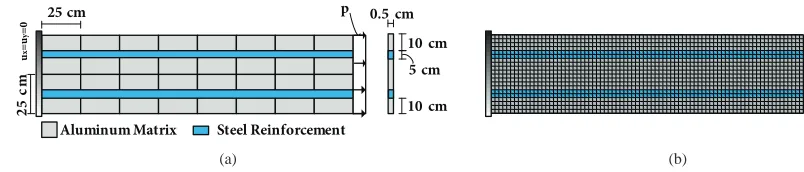
Fig. 4. (a)Model Definition(b)Finite Element mesh

is considered, reinforced with two steel strips (Fig.4(a)). The length, width and height of the beam areLm = 200cm,

bm= 0.5cmandhm= 50cmrespectively. The height of the steel strips ishf = 5cm. The constituents are assumed to be elastic-perfectly plastic with deterministic Poisson ratiosνa= 0.33andνs= 0.3for the aluminum and steel respectively.

Non Degrading material For verification purposes, no damage is considered in this case setting and the results of the proposed multiscale formulation are compared to results derived by running the fine meshed model in Abaqus commercial code64. The elastic moduli and the corresponding yield stresses of the materials are considered to be random variables. The Log-Normal distribution is used for all random variables with corresponding mean values Ema = 70GP a and

fya = 214M P afor the aluminum andEms = 200GP aandfys = 235M P afor the steel. The following deterministic load is considered

p(t) = 20000tsin(πt)kP a

The fine meshed finite element model, presented in Fig.4(b),consists of 1600 linear quadrilateral plane stress elements with a total of 3358 free degrees of freedom. The multiscale finite element model is formulated by 16 plane stress coarse elements. The corresponding representative RVE consists of 100 plane stress elements. The periodic boundary condition assumption is used to evaluate the micro-basis interpolation functions.

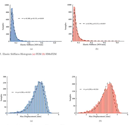
A total 5000 Monte Carlo iterations is performed for the FEM and HMsFEM case and by considering a Latin Hypercube sampling scheme. It should be stressed that different random seeds and, as a result, different sets of random variables are used for each model class, in order to obtain an unbiased comparison. The derived data sets of the effective elastic stiffness evaluated from the response of the FEM and HMsFEM analysis cases are presented in Fig5(a)and5(b)respectively. This effective value is calculated as the slope of the elastic region of the force-displacement diagram for the first cycle of loading. Furthermore, the histograms of the maximum displacements are presented in Fig.6, providing in this way a measures that quantifies structural response under loads that push the system into the plastic region, thereby serving as a tool for assessing structural reliability. In both cases, the relative deviation between the statistical parameters of the corresponding parametric PDEs is lower than 0.5%.

Degrading material In this case, the variability of the strength deterioration and stiffness degradation parameters is also considered. To better illustrate their effect on the dynamic response of the structure, the following, constant amplitude, sinusoidal excitation is considered in this case

p(t) = 250000sin(πt)kP a

0.2 0.4 0.6 0.8 0

200 400 600 800 1000

Elastic Stiffness [MN/mm]

Samples

κ=0.389, μ=0.135, σ=0.019

(a)

0.2 0.4 0.6 0.8

0 200 400 600 800 1000

Elastic Stiffness [MN/mm]

Samples

κ=0.394, μ=0.133, σ=0.019

(b)

Fig. 5. Elastic Stiffness Histogram(a)FEM(b)HMsFEM

1 2 3 4 5 6

0 50 100 150 200 250 300

Max Displacement [mm]

Samples

μ=4.220, σ=0.523`

(a)

1 2 3 4 5 6

0 50 100 150 200 250

Max Displacement [mm]

Samples

μ=4.250, σ=0.524

(b)

Fig. 6. Maximum Displacement Histogram(a)FEM(b)HMsFEM

Variable Min Max

Ema 62500000 kPa 67500000 kPa

fya 200000 kPa 242000 kPa

cηm 2.5e-7 2.5e-6

csm 5.0e-7 5.0e-6

Es 200000000 kPa 231000000 kPa

fys 225000 kPa 247500 kPa

cηs 2.5e-7 2.5e-6

css 5.0e-7 5.0e-6

-800

-600

-400

-200

0

200

400

600

800

-150

-100

-50

0

50

100

150

T

o

ta

l

A

p

pl

ie

d

F

o

rc

e

(K

N

)

Displacement (mm)

FEM

HMsFEM

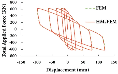
Fig. 7. Degrading Material: Force Displacement Loops (Mean Values)

In Fig.7, the total applied force versus the center-point axial displacement at the tip of the cantilever is presented. The results obtained from the two procedures are practically identical. In this case, the analysis conducted using the HMsFEM procedure concluded in 900 sec while the corresponding analysis time using the standard FEM procedure was 4626 sec, amounting to a significant reduction in the computational toll involved.

In this case 2000 Monte Carlo simulations were performed for each one of the solution approaches. Contrary to the case examined in the non-degrading material case,the same pool of random variables is considered for both cases. The derived results are again compared in terms of the estimated PDFs of the response variables.

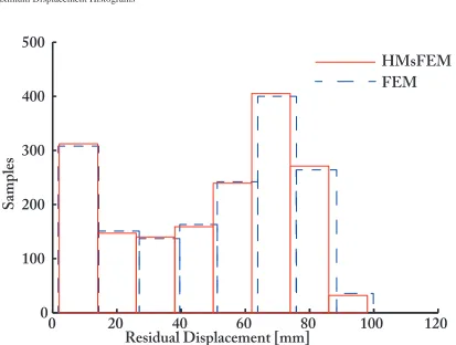
In Fig.8the histograms of the derived maximum displacements are presented for the case of the HMsFEM and FEM analysis respectively.The HMsFEM approach results in a marginally stiffer configuration as compared to the FE method. The same trend is also revealed form the histograms of the residual displacement presented in Fig.9for the multiscale and finite element methods respectively. This discrepancy is due to the approximate nature of the micro to macro interpolation scheme introduced in relation (5) and the numerical implementation of the periodic boundary condition assumption introduced on the coarse elements. The divergence from the “exact” finite element model is less than 2%. The mathematical framework of the multiscale finite element method41_{provides appropriate theorems to verify that this error is bounded.}

6.2. Inverse Problem Formulation

0

100

200

300

400

500

600

0

200

400

600

800

1000

Max Displacement [mm]

Samples

HMsFEM

FEM

Fig. 8. Maximum Displacement Histograms

0

20

40

60

80

100

120

0

100

200

300

400

500

Residual Displacement [mm]

Samples

HMsFEM

FEM

25 cm

2

5

c

m

Aluminum Matrix

Steel Reinforcement

Coarse

Element

Acceleration sensor

Mass

m

=15tn

p(t)

Fig. 10. Acceleration sensor locations

0

5

10

15

20

−200

−100

0

100

200

300

time [sec]

Applied

P

ress

ure [MPa]

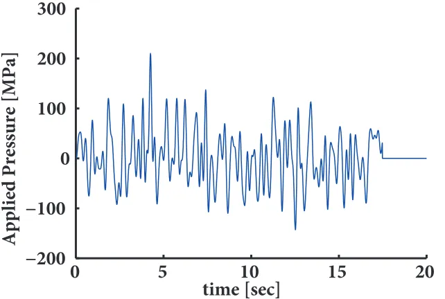
Fig. 11. Time history plot of the randomly generated input load.

and height ofLm = 200cm,bm= 0.3cmandhm = 50cmrespectively. The height of the steel strips ishf = 5cm. A concentrated mass of15tnis attached on the free end of the beam. A random pressure load is applied at the free end of this setup. The loadp(t)is obtained via filtering a white noise processwp(t)∼N ID(0, σ2

e), with NID denoting a Normally

Independently Distributed process with the indicated mean and variance.wp(t)is filtered using a low-pass filter with a

5Hzcut-off frequency. This type of load, illustrated in Figure11, allows for the simulation of a simple testing procedure driven by means of a suitable shaker device with an appropriate stinger, exerting an axial load on the lumped15tnmass.

The goal is to utilize information from the structure in the form of acceleration measurements obtained at a finite set of sensor locations, nine in total, as indicated in Figure 10, in order to identify the properties of the constituents involved. The four constitutive parameters, namely the elastic stiffness and yield stress of each of the two constituents, are considered as unknown a-priori or, more precisely, as uncertain. An “off" initial assumption is made on the values of these parameters, which is utilized as the initial condition to be fed into the UKF algorithm. The corresponding initial values are

θ0_{1=Ema= 87.5GP a},θ0_{2=fya= 267.5M P a}for the aluminum andθ0_{3=Ems= 241.5GP a},θ0_{4=fys= 211.5M P a}

0

5

10

15

20

−100

−50

0

50

100

time [sec]

Vel

ocity [mm/sec]

UKF estimation

Actual

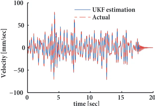
Fig. 12. Observed Node 3 velocity time-history estimate (blue) versus actual value (red).

A reference forward analysis is performed in ABAQUS, employing a fine mesh; this serves as the “actual” response, utilized here as the equivalent of an experimental testing process. Therefore, the measurement vectory_k, comprising nine acceleration data sets to be fed into equation (54) of the UKF, is herein generated via an independent numerical simulation. The crucial component lies in the utilization of the forward (or process) model for the UKF. As explained earlier, the UKF is formulated using a discrete set of samples, termed the Sigma Points. The number of these Sigma Points equals

2∗L+ 1, whereLis the size of the augmented state of the system. For a joint state-parameter identification problem, this augmented vector comprises the system’s displacements and velocities at every degree of freedom, as well as the unknown parameters (four in this example). It therefore becomes evident, that if one is to utilize a finely meshed model construed in ABAQUS, the dimension of the system would be too large for numerical computation. Even more importantly, due to memory limitations, there exists a critical matrix size, and therefore an associated mesh refinement, for which calculations would be prohibited.

A means for solving this problem is delivered through the proposed HMsFEM approach. In what follows, the process and observation functions denoted asF,H in (54) are substituted by the HMsFEM solver between successive time steps. A coarse mesh of 24 nodes is utilized, bringing the state dimension down to a dimensionL = 2∗24 + 4 = 52. The corresponding Sigma Point set therefore comprises a total of2L+ 1 = 105components. Furthermore, the Sigma Point analyses are in fact independent, allowing for the parallel execution of these forward runs. The identification process is consequently initiated with the following settings for the filter. An initial covariance of the state,P_x, of the order of1e−13

is assigned. The process and observation noise covariance matrices,Qk andRk respectively, are set as a diagonal with

diagonal components equal to1e−13and1e−5correspondingly. For facilitating the filter implementation, and avoiding numerical errors, the parameter values are normalized with a target values set at 0.01 for all four constitutive parameters.

The results of the identification process are summarized in Figures 12-15. Figures 12-13summarize the velocity predictions of the filter for both an observed (node #3), i.e., monitored via a virtual sensor, as well as an unobserved (node #21) degree of freedom. It is noted that in both cases, the filter furnishes a very accurate estimation of the corresponding nodal velocities. Nonetheless, an integration error, which can also be related to the selected level of process noise, is noticeable in the displacement estimates. This accumulation of integration errors resulting in displacement drifts is not uncommon in system identification, as noted in65_{, nonetheless this does not create a hindrance in the particular inverse}

0

5

10

15

20

−20

−10

0

10

20

30

time [sec]

Vel

ocity [mm/sec]

UKF estimation

Actual

Fig. 13. Unobserved Node 21 velocity time-history estimate (blue) versus actual value (red).

0

5

10

15

20

−8

−6

−4

−2

0

2

4

time [sec]

Displacement [mm]

UKF estimation

Actual

0

5

10

15

20

−2

−1.5

−1

−0.5

0

0.5

1

time [sec]

Displacement [mm]

UKF estimation

_Actual

Fig. 15. Unobserved Node 21 displacement time-history estimate (blue) versus actual value (red).

The primary target of this inverse formulation is the extraction of the true parameters that characterize the structural properties, i.e., the stiffness and strength characteristics. Figure16indicates the convergence of the parameter estimation to the true, “normalized” parameter value which is set to 0.01 (unitless) for all time-invariant variables involved. The successful utilization of the filter is enabled through the implementation of the proposed multiscale scheme. For the purpose of comparison, it is mentioned that on a PC fitted with an Intel i7 processor and 32 GB of RAM, utilizing all 4 cores, the time allocated for the analysis was approximatelly 4 hrs. If the ABAQUS model were to be employed using the Finite Element mesh presented in Figure4(b), a prohibitive total time of 4 days would be delivered. It is therefore pointed out, that the appropriate combination of advanced modeling tools with appropriate identification and uncertainty quantification techniques enables the validation of computational mechanics models seeking to accurately reproduce structural response. This is of particular significance in the case of nonlinear hysteretic response, where the cost of computation forms a major concern.

7. Conclusions

0

5

10

15

20

0.0085

0.009

0.0095

0.01

0.0105

0.011

0.0115

0.012

time [sec]

Normal

is

ed Parameter Value

E

E

f

E

Fig. 16. Constitutive parameters estimates versus the reference (normalized) value (black line).

process can grease the wheels of the process chain from design, through manufacturing and production, to operation and maintenance.

8. Acknowledgments

This work has been supported by the Swiss National Science Foundation under grant#200021_146996 for the “Hysteretic Multi/Scale Modeling for the Reinforcing of Masonry Structures”. The authors are also grateful to the University of Nottingham for access to its high performance computing facility.

References

[1] Strong AB. Fundamentals of Composites Manufacturing, Methods and Applications. 2nd ed. MI: Society of Manufacturing Engineers,

Dearborn; 2008.

[2] Rohatgi P. Low-cost, fly-ash-containing aluminum-matrix composites. JOM. 1994;46(11):55–59.

[3] Saheb DN, Jog JP. Natural fiber polymer composites: A review. Advances in Polymer Technology. 1999;18(4):351–363.

[4] Peng X, Fan M, Hartley J, Al-Zubaidy M. Properties of natural fibre composites made by pultrusion process. Journal of Composite

Materials. 2011;.

[5] Munch E, Launey ME, Alsem DH, Saiz E, Tomsia AP, Ritchie RO. Tough, Bio-Inspired Hybrid Materials. Science.

2008;322(5907):1516–1520.

[6] Belingardi G, Beyene AT, Koricho EG. Geometrical optimization of bumper beam profile made of pultruded composite by numerical

simulation. Composite Structures. 2013;102(0):217 – 225.

[7] Jauregui R, Silva F. Numerical Validation Methods, Numerical Analysis - Theory and Application. Prof Jan Awrejcewicz (Ed),

InTech. 2011;.

[8] Oreskes N, Shrader-Frechette K, Belitz K. Verification, Validation, and Confirmation of Numerical Models in the Earth Sciences.

Science. 1994;263(5147):pp. 641–646. Available from:http://www.jstor.org/stable/2883078.

[9] Patterson EA, Feligiotti M, Hack E. On the integration of validation, quality assurance and non-destructive evaluation. The Journal

[10] Felipe-Sesé L, Siegmann P, Díaz FA, Patterson EA. Simultaneous in-and-out-of-plane displacement measurements using fringe

projection and digital image correlation. Optics and Lasers in Engineering. 2014;52(0):66 – 74.

[11] Burguete RL, Lampeas G, Mottershead JE, Patterson EA, Pipino A, Siebert T, et al. Analysis of displacement fields from a high-speed

impact using shape descriptors. The Journal of Strain Analysis for Engineering Design. 2013;.

[12] Soares CMM, de Freitas MM, Araújo AL, Pedersen P. Identification of material properties of composite plate specimens. Composite

Structures. 1993;25(1⣓4):277 – 285.

[13] Frederiksen P. Experimental procedure and results for the identification of elastic constants of thick orthotropic plates. Journal of

Composite Materials. 1997;31:360–382.

[14] Rikards R, Chate A, Steinchen W, Kessler A, Bledzki AK. Method for identification of elastic properties of laminates based on

experiment design. Composites Part B: Engineering. 1999;30(3):279 – 289.

[15] Tucker CLI, Erwin L. Stiffness predictions for unidirectional short-fiber composites: Review and evaluation. Composites Science

and Technology. 1999;59(5):655 – 671.

[16] Aboudi J. Micromechanics of Composite Materials. Butterworth-Heinemann, Oxford; 2013.

[17] Maletta C, Pagnotta L. On the determination of mechanical properties of composite laminates using genetic algorithms. International

Journal of Mechanics and Materials in Design. 2004;1(2):199–211.

[18] Ekel’chik VS. Resonance methods for determining the complex shear moduli of orthotropic composites. Mechanics of Composite

Materials. 2007;43(6):487–502.

[19] Abrosimov NA, Kulikova NA. Parameter identification in viscoelastic strain models for composite materials by analyzing impulsive

loading of shells of revolution. Mechanics of Solids. 2011;46(3):368–379.

[20] Bažant ZP, Daniel IM. Size Effect and Fracture Characteristics of Composite Laminates. Journal of Engineering Materials and

Technology. 1996;118(3):317–324.

[21] Liu D, Raju BB, Dang X. Size effects on impact response of composite laminates. International Journal of Impact Engineering.

1998;21(10):837 – 854.

[22] Pickett AK. Review of Finite Element Simulation Methods Applied to Manufacturing and Failure Prediction in Composites Structures.

Applied Composite Materials. 2002;9(1):43–58.

[23] Hansun TT. Homogenization of dynamic laminates. Journal of Mathematical Analysis and Applications. 2009;354(2):518 – 538.

[24] Pahlavanpour M, Moussaddy H, Ghossein E, Hubert P, Lévesque M. Prediction of elastic properties in polymer⣓clay

nanocom-posites: Analytical homogenization methods and 3D finite element modeling. Computational Materials Science. 2013;79(0):206 –

215.

[25] Nguyen VP, Stroeven M, Sluys LJ. An enhanced continuous–discontinuous multiscale method for modeling mode-I cohesive failure

in random heterogeneous quasi-brittle materials. Engineering Fracture Mechanics. 2012;79(0):78 – 102.

[26] Geers MGD, Kouznetsova VG, Brekelmans WAM. Multi-scale computational homogenization: Trends and challenges. Journal of

Computational and Applied Mathematics. 2010;234(7):2175–2182.

[27] Efendiev Y, Ginting V, Hou T, Ewing R. Accurate multiscale finite element methods for two-phase flow simulations. J Comput Phys.

2005;.

[28] Babuška I. Homogenization approach in engineering; 1975. ORO–3443-58; TN-BN–828 United States; NSA-33-022692.

[29] He X, Ren L. Finite volume multiscale finite element method for solving the groundwater flow problems in heterogeneous porous

media. Water Resources Research. 2005;41(10):1–15.

[30] Zhang HW, Wu JK, Lv J. A new multiscale computational method for elasto-plastic analysis of heterogeneous materials.

Computational Mechanics. 2012;49(2):149–169.

[31] Triantafyllou SP, Chatzi EN. A hysteretic multiscale formulation for nonlinear dynamic analysis of composite materials.

Computational Mechanics. 2014;54(3):763–787.

[32] Triantafyllou S, Koumousis V. Hysteretic Finite Elements for the Nonlinear Static and Dynamic Analysis of Structures. Journal of