Metastable decoherence free subspaces and electromagnetically induced transparency in interacting many body systems

in interacting many-body systems

Katarzyna Macieszczak,1, 2 _{YanLi Zhou,}3 _{Sebastian Hofferberth,}4

Juan P. Garrahan,1, 2 _{Weibin Li,}1, 2 _{and Igor Lesanovsky}1, 2

1_{School of Physics and Astronomy, The University of Nottingham, Nottingham, NG7 2RD, United Kingdom} 2

Centre for the Mathematics and Theoretical Physics of Quantum Non-equilibrium Systems, University of Nottingham, Nottingham NG7 2RD, UK

3_{College of Science, National University of Defense Technology, Changsha, 410073, China} 4

Department of Physics, Chemistry and Pharmacy, University of Southern Denmark, Odense, Denmark

We investigate the dynamics of a generic interacting many-body system under conditions of elec-tromagnetically induced transparency (EIT). This problem is of current relevance due to its connec-tion to non-linear optical media realized by Rydberg atoms. In an interacting system the structure of the dynamics and the approach to the stationary state becomes far more complex than in the case of conventional EIT. In particular, we discuss the emergence of a metastable decoherence free subspace, whose dimension for a single Rydberg excitation grows linearly in the number of atoms. On approach to stationarity this leads to a slow dynamics which renders the typical assumption of fast relaxation invalid. We derive analytically the effective non-equilibrium dynamics in the deco-herence free subspace which features coherent and dissipative two-body interactions. We discuss the use of this scenario for the preparation of collective entangled dark states and the realization of general unitary dynamics within the spin-wave subspace.

I. INTRODUCTION

The phenomenon of electromagnetically induced trans-parency (EIT) is currently extensively studied both theo-retically and experimentally [1–3]. It finds applications in the context of quantum memories [4, 5] and slow light [6] as well as in the mediation of effective photon-photon in-teractions [7–13]. These are important ingredients for op-tical quantum computing and permit the creation of non-linear optical elements such as single-photon switches and transistors [14–19], single-photon absorbers [20], as well as photon gates [21].

In the context of EIT a common assumption is made concerning a separation of timescales between the slow propagation of the optical fields and the fast dynamics of the atomic medium. The latter is therefore assumed to be always in its stationary state and the transmission properties of the atomic medium are determined by the corresponding stationary state density matrix.

In this work we show, however, that the dynamics of an interacting atomic medium is not necessarily fast due to the emergence of quantum metastability [22]. To illus-trate this we explore analytically the long-time evolution of a generic interacting many-body ensemble under EIT conditions. We demonstrate that the effective dynamics in fact takes place within a metastable decoherence free subspace (DFS) of spin-waves (SWs), and features both dissipative and coherent two-body interactions [23]. The emerging slow timescales lead to a violation of the typi-cal assumption of fast system relaxation [1] which dras-tically affects the system’s (non-local) optical response. We show analytically that the effective long-time dynam-ics can be employed for preparing stationary pure and entangled SW dark states [24–27], and, in the limit of

weak interactions, allows to implement arbitrary unitary evolution within the metastable DFS [28, 29]. Our study is relevant for recent investigations in the context of Ry-dberg quantum optics, but more generally sheds light on non-trivial effects due to quantum metastability in inter-acting many-body systems.

The structure of the paper is as follows. In Sec. II we introduce a generic interacting many-body system in EIT configuration. In Sec. III we discuss its metastable states and in Sec. IV derive the effective long-time dynamics. In Sec. V we study the optical response of the system. Finally, in Sec. VI we discuss stationary states of the ef-fective dynamics and show how the dynamics can be used for pure entangled state preparation, as well as realisa-tion of universal unitary gates (Sec. VII). The results of the paper are summarized in Sec. VIII.

II. THE SYSTEM

We consider the dynamics of a system ofN interacting atoms with four relevant electronic levels, as depicted in Fig. 1a: the ground state_|1_i, a low-lying short-lived ex-cited state_|2_iand two long-lived states_|3_iand_|4_i. The |1i ↔ |2i-transition is driven by a (weak) probe field with Rabi frequency Ωp(r, t), while the|2i ↔ |3i-transition is coupled by a (strong) control laser field with Rabi fre-quency Ωc(r), giving rise to a typical EIT configuration. Within the dipole and rotating wave approximations, the laser-atom coupling Hamiltonian is

Hj =X n=2,3

δnσj nn+

Ωp(rj, t)σj₂₁+ Ωc(rj)σ32j + h.c.

DFS

⌦p

⌦c

|

1

_i

|

2

i

|

3

i

|

4

_i

3

2

k

(a)

(b)

(c)

{

-0.1

-0.2

j

⌦p

⌦c

Metastable DFS ⌦p

⌦c

|1_{· · ·}1j_{· · ·}4k_{· · ·}1_i |1· · ·4j· · ·1k· · ·1i

|1· · ·4j· · ·2k· · ·1i |1· · ·4j· · ·3k· · ·1i

|1_{· · ·}2j_{· · ·}4k_{· · ·}1_i |1· · ·3j· · ·4k· · ·1i Ujk

⌦p

⌦c

|

1

i

|

2

_i

|

3

_i

|

4

i

3

2

⌧

Ujk

Re( )

1

×102

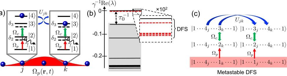
FIG. 1. Metastable DFS of anN-atom system: (a) Level scheme and transitions. (b) Spectrum of the master operator

Ldisplaying a separation of eigenvalues between low-lying modes (λ1 = 0, λ2, ..., λN2) (full and dashed) corresponding to the

long-time dynamics in Eq. (6), and fast modesλk>N2 (shaded). Data forN = 3 atoms with van der Waals interactions on a

one-dimensional lattice (lattice spacinga), dispersion coefficientsC34= 1.3×γa6 _andCex=γa6_{, in the presence of uniform}

fields Ωp= Ωc/50 =γ/50 and the detuningδ2=δ3= 0. (c) Exchange interactionsUjktogether with the probe-field coupling lead to a slow non-local dynamics within theN-dimensional DFS of spin-waves, and render it metastable.

where σ_abj =|ajihbj|and δn(n= 2,3) are the detunings of the respective lasers.

Atoms interact via the density-density interaction

Vjk= X

n,m=3,4

Vnm

jk σjnnσkmm (2)

and the exchange interaction Ujk=Ujk34σ

j

43σk34+ h.c.. (3)

Interactions among the low-lying states, _|1_iand _|2_i, are neglected. This choice is rather generic, but also mo-tivated by recent investigations of EIT within Rydberg gases [15–17, 20, 30, 31], where the upper states|3iand |4icorrespond to two different Rydberg levels: two Ry-dberg atoms, located at positionsrj andrk, interact via van der Waals interactionVmn

jk =Cmn/|rj−rk|6, and ex-change interactionU34

jk =Cex/|rj−rk|6, with dispersion coefficientsCex,C33,C44, andC34=C43[31–33].

Coherent dynamics is supplemented by dissipative de-cay of the short-lived state_|2_iinto the ground state_|1_iat rateγ. The evolution of the density matrixρis governed by a quantum master equation, with master operatorL, given by [34, 35]

d

dtρ=Lρ=−i[H, ρ] +γ N

X

j=1

D(σ12j )ρ, (4)

with the dissipator_D(L)ρ:=LρL†

−1 2{L

†_{L, ρ}

} and the HamiltonianH =PN

j=1Hj+

PN

j>k[Ujk+Vjk].

III. METASTABLE MANIFOLDS

Metastable manifolds in non-interacting EIT. It is in-structive to first consider the non-interacting case in or-der to get an idea of the resulting decoherence free sub-space (DFS), the emergence of metastability and the cor-responding timescales. In the absence of interactions

state|4iis dynamically disconnected from the remaining levels, cf. Fig. 1a, and each atom possesses two stationary states: a mixed stateρss,r supported on the lower three

levels, and the pure non-decaying excited state_|4_ih4_|. An interesting situation occurs when both stationary states are pure, i.e. ρss,r 7→ |ψrihψr|. It follows that

|ψri is a so-called dark state, i.e. σ12|ψri = 0, and

also an eigenstate of the local Hamiltonian, Hr|ψri =

Er|ψri[26, 27]. Therefore, also coherences between|ψri

and |4i become stationary, so that |ψri and |4i span a

DFS. On resonance, i.e. δ3= 0, we have

|ψri=

Ω∗

c(r)|1i −Ωp(r)|3i

p

|Ωc(r)|2_+|Ωp(r)|2, (5)

and the dark stationary state is reached on a timescale τ0, determined by the spectral gap of the master

opera-tor _L, cf. Fig. 1b. For small non-zero detuning δ3, the

single-atom DFS, spanned by_|ψriand |4i, is no longer

truly stationary, but becomes metastable [22], as the sta-tionary state degeneracy is partially lifted and low-lying slow modes appear in the spectrum of L, see Fig. 1b. These modes govern the long-time dynamics within the DFS at t & τ = _O[1/(δ2

3τ0)], which relaxes the system

to the actual stationary state, i.e. a mixture ofρss,rand

|4ih4|[36].

When using EIT to control light fields, e.g. for quantum memories or light storage, the response of the atomic ensemble to the incident field Ωp(rj, t) is determined by the coherence between the low-lying states _|1_i and _|2_i, _hσ12iss, calculated in the stationary

stateρss,r[1]. This implicitly assumes that the timescale

τp connected to the probe field dynamics, is significantly longer than the relaxation timeτ0 of the atomic

ensem-ble, defining an adiabaticity condition. At resonance, δ3= 0, the ensemble then remains in the dark state|ψri

by adiabatically following Ωp(r, t), thereforehσ12iss = 0,

relaxation time τ can in principle become arbitrarily long. The answer is that the coherence relaxes to its stationary value, _hσ12iss, at the fast timescaleτ0 τp,

as the slow dynamics related to τ corresponds to dephasing of coherences between |ψri and |4i, which

are irrelevant for the optical response. Thus, although the non-interacting system for δ3 6= 0 becomes in fact

metastable, this does not invalidate the adiabaticity condition.

Metastable manifolds of the interacting system. In the presence of interactions, in particular the long-range ex-change interaction Ujk, this no longer holds true. Here a slow collective dynamics within a metastable DFS emerges which affects the optical response by introducing a new timescale that becomes relevant for EIT.

To study this in detail, we note that in the ab-sence of the probe field, the ground level _|1_i is discon-nected from the dynamics, as shown in Fig. 1a. For a single atom also the level |4i is disconnected. For many atoms this is no longer the case, but the ex-change and density-density interactions connect_|4j_ionly to _|3k_ior _|4k_i, and thus states_|1j4k_iare left invariant, Ujk_|1j4k_i= 0 =Vjk_|1j4k_i, while_|4j4k_igain phase due to Vjk_|4j4k_i=V44

jk|4j4kiandUjk|4j4ki= 0. Therefore, the manifold of non-decaying states of N interacting atoms is a 2N_{-dimensional DFS of atoms either in |1i or |4i.} In this work we consider the case in which initially only a single atom is found in state_|4_i, which is particularly relevant in the context of recent experiments with Ryd-berg gases [15–17, 20, 30, 31]. Here, since the dynam-ics (4) conserves the number of atoms in|4i, stationary states form a N-dimensional DFS, spanned by localised excitations _|j_i := _|11· · ·1j−14j1j+1· · ·1Ni, or

equiva-lently SWs|Ψ(ks)i=N−1/2PN

j=1eiks·rj|ji, as shown in

Fig. 1c. Once the weak probe field is switched on, this DFS becomes metastable [22]. On the level of the master operator _L [Eq. (4)] this means that the firstN2

eigen-modes no longer have strictly zero eigenvalue, but still are separated from the rest of rapidly decaying modes, as sketched in Fig. 1b. The dynamics within this metastable DFS, represented by the low-lying modes, then appears stationary at timescales much longer than the relaxation time τ0,int of the fast modes, which coincides with the

system relaxation in the absence of the probe field, cf. the non-interacting case above.

IV. EFFECTIVE EQUATIONS OF MOTION

In the following we characterize the dynamics within the metastable DFS, which we calculate analytically to leading order in the probe field strength [22, 37], see Ap-pendices B and A. For the sake of simplicity we con-sider here a control field of the form Ωc(r) = eikc·r|_Ωc|

and isotropic density-density interactions, V34

jk = Vkj34. Within the metastable DFS the density matrixρevolves

2500

5000

7500

0.85 0.9 0.95 1 1.05 1 2 3

5 10 15 20 25 30 5

10

15

20

25

30

5 10 15 20 25 30 100

200

300 400 500 600 700

x (a)

k

(d)

t

(e)

(d) (f)

(c)

(b)

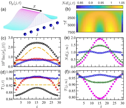
FIG. 2. Long-time dynamics and optical response: (a) Stationary Gaussian probe field Ωp(j) propagating perpen-dicular to a chain of N = 30 atoms with van der Waals interactions, initially in a SW with ks = 0. (b) Dynam-ics of the density d(j, t) of a single |4i-excitation. The in-terplay between coherent and dissipative hoping leads to a double-peak density distribution, strikingly distinct from the uniform density of the non-interacting case. (c) The station-ary densityd(j,∞) for lattice spacinga0 =a (#),a0 = 0.9a

(•), a0 = 0.8a ( ). In the limit of strong interaction the stationary density follows the probe field intensity profile as

ρss∝PNj=1|Ωp(rj)|2|jihj|. (d) The polarisation Imhσj21(t)iat

timest= 100γ−1 (3),t= 1000γ−1 (M) andt= 7500γ−1(#). At all times polarisation is distinct from a Gaussian profile that would be observed in the non-interacting case (orange dashed line forUjk= 0). (e) Exchange interactions lead to a non-uniform transmission profile of the probe field transmis-sionT(j, t) [cf. (d) for labels]. (f) The stationary transmis-sionT(j,∞) [cf. (c) for labels] becomes dependent only on the field intensity for strong interactions, see Eq. (13). The probe field profile is Ωp(j) = Ω0exp[−a02(j−jc)2/2l2] with its centerjca0coinciding with the chain center, widthl= 8a0 and Ω0= Ωc/20 =γ/20. Other parameters as in Fig. 1b.

according to the master equation

d dtρ=

N

X

j=1



−i 



N

X

k>j Hjk, ρ



+D(Lj)ρ 

. (6)

The perturbative Hamiltonians are given by

Hjk=ωzjk|jihj|+ωkjz |kihk|+

ωxyjk|jihk|+ h.c.

,(7)

with the frequencies

ωzjk=|Ωp(rk, t)|2Im(αjk), (8)

ω_jkxy=eikc·(rj−rk)_{Ωp(rj, t) Ω}∗

p(rk, t)

βjk−β∗

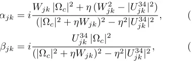
where

αjk=iWjk|Ωc|

2_+η(W2

jk− |Ujk34|2) (_|Ωc_|2_+ηWjk)2_−η2_|U34

jk|2

, (10)

βjk=i U

34

jk|Ωc|2 (_|Ωc_|2_+ηWjk)2_−η2_|U34

jk|2

, (11)

withη:=−δ2+iγ₂ andWjk :=δ3+Vjk34. These param-eters also enter the jump operators,

Lj =√γ N

X

k6=j

eikc·rj_{Ωp(rj, t)αkj}

|k_ihk_| +

+eikc·rk_{Ωp(rk, t)βkj|kihj|, (12)}

which correspond to a dissipative decay of an (j-th) atom to its ground state after a low-energy excitation is introduced to the system by the probe field. Note that effective dissipative processes within the DFS are in general dependent on coherences between distant sites.

When the exchange interaction is zero, Ujk = 0, we haveβjk= 0 and the jump operators (12) lead to dephas-ing between localised excitations, similarly as in the non-interacting case, but with the rates modified by density-density interactions. In contrast, a finite exchange in-teraction introduces non-local dynamics, through both coherent and dissipative processes. To illustrate this, we study the evolution of the local densityd(j, t) =_hj_|ρ(t)_|j_i, of atoms in state _|4_i under the action of a probe field propagating in the direction perpendicular to an atom chain (z-axis), as shown in Fig. 2a. The field has a sta-tionary Gaussian profile. The exchange interaction leads to spatially dependent dynamics of excitations, as the non-uniform field breaks the translation symmetry. As a consequence, for moderate interaction strengths the exci-tation density dynamically develops a double peak struc-ture from an initially uniform distribution when V34

jk + δ3 > Ujk34 (Fig. 2b), while for strong interactions classi-cal detailed balance dynamics emerges, see Appendix C, leading to the stationary state approximately following the probe field profile, ρss _{≈ N}−1PN

j=1|Ωp(rj)|2|jihj|,

whereN =PN

j=1|Ωp(rj)|2, see Fig. 2c.

V. OPTICAL RESPONSE

Let us now study the optical response. For an initial stateρlying within the single-excitation DFS, the optical response is determined by the polarization

hσ12j (t)i=−iΩp(rj, t)

N

X

k6=j

αjkρkk+ (13)

−i N

X

k6=j

eikc·(rk−rj)_{Ωp(rk, t)βjkρjk+O |Ωp(rk, t)τ} 0,int|3,

whereρjk =hj_|ρ(t)|k_iare coherences between |4i- exci-tations of different atoms, cf. [32, 33]. Compared to the response encountered in conventional EIT [1], there are two differences. First, there are non-local contributions, i.e. the response of one atom generally depends on all others. Second, the coherenceρjk evolves slowly within the metastable manifold, indicating the emergence of a non-equilibrium polarization.

These effects can be seen in Fig. 2d, where we show the imaginary part of the polarization and observe a slow change, on a timescale _∝ 1/[_|Ωp(rj)_|2_τ

0,int] [38], from

its metastable value to the stationary one. Note, that the timescale corresponding to each atom is not sim-ply monotonically dependent on the probe field Ωp(rj) due to non-local exchange of the coherence and probe field, cf. Eq. (13). In Rydberg experiments, sig-natures of this physics can be probed through the transmission signal of the probe light as shown in Fig. 2e,f. Here we show the transmission T(j, t) = ∆t−1|Ωp(rj)|−2Rt+∆t

t dt

0

|Ω(out)p (rj, t0)|2 with ∆t =γ−1. In Fig. 2e we observe that the signal changes from the initial Gaussian profile to a significantly flatter one at later times. At all times the signal is strikingly different from the uniform and time-independent transmission in the non-interacting case. For stronger interactions the stationary transition simply decreases with the increas-ing intensity of the probe field, see Fig. 2f.

VI. STATIONARY STATES OF THE INTERACTING SYSTEM

The stationary state of the long-time dynamics of Eq. (6) corresponds to the stationary stateρss of the full

dynamics of Eq. (4) [22]. Without exchange interactions, the long-time dynamics leads to dephasing of coherences between localised excitations|j_i. For an initial state with a single excitation in state |4i there are thus N possi-ble stationary states, with any SW decaying to the fully mixed state,ρss =N−1PNj=1|jihj|+O(Ωp(t)τ0) [39].

To gain some analytic insights into the case of non-zero exchange interactions we consider the cases of all-to-all and nearest-neighbour (NN) interactions. In the former case,αjk=αandβjk=β, which in the presence of the uniform probe field, Ωp(r, t) =eikp·r_{|Ωp(t)|, leads to the}

unique and uniform stationary state,

ρss=N−1

N

X

j=1

|j_ihj_|+cN N

X

k6=j

ei(kp+kc)·(rj−rk)_|jihk|,

wherecN = [(N₋2)_|β_|2

−2Re(α∗_β)]/[(N

−1)_|β_|2₊

|α_|2_].

For a finite numberN >2 of atoms,ρss is mixed unless

5 10 50 100 10-7

10-6

10-5

10-4 - /

-5 0 5 10 15 20 25

2

36 30 24 18 12 6

N

0.2 0.3 0.4 0.5 0.6 0.7 0.8 0.9

-10 0 10 20 30

N 40

30

20

10

0.9

0.7

0.5

0.3

-10 0 10 20 30 /

1 2 3 4 5 6

- / ×

(a) (b)

(d)

(c)

-10 0 10 20 30 /

10-4

10-5

10-6

10-7 - /

5 10 20 50

0.98 0.99 1.00

FIG. 3. Spectral gap and pure stationary state: (a) Scaling of the spectral gap for an open chain ofN atoms with nearest-neighbour (NN) () and van der Waals (vdW) inter-actions (_#) atδ2= 0. The gap is compared with the scaling

π2_Γ/N2 _{(red dashed lines) andπ}2_Γ/N2_{+ 8Γ}(1) _{(blue dashed}

lines), where Γ =γ|Ωp|2|αj,j+1|2 and Γ(1)=γ|Ωp|2|αj,j+2|2, see Appendix D for discussion. (b) The overlaphΨss|ρss|Ψssi of the stationary state with (14) for a system with vdW inter-actions. The overlap decays with growingN due to the tails in vdW interactions, but for eachN the detuning δ2 can be chosen to maximise the overlap. Vertical cut through panel (b) atδ2 = 3γ is shown in (c). (d) The spectral gap depen-dence on the detuning δ2 for N = 20 atoms ( with NN, #with vdW interactions). The largest spectral gap, which is well approximated by π2Γ/N2 and π2Γ/N2+ 8Γ(1) (red and blue dashed lines), corresponds to the maximal overlap in (b), thus giving the optimal δ2 ≈ |Ωc|2/[2Uj,j34+1] when

Γ≈ |Ωp|2/γ. In these simulations the dispersion coefficients are C34 =Cex = 1.3×γa6 and the lattice spacing is √2a. The fields are uniform Ωp= Ωc/20 =γ/20 andδ3= 0.

|U34

j,j+1|=|Vj,j34+1|,δ3= 0,

|Ψssi=N−1/2

N

X

j=1

(₋1)jΩp(e rj)|ji, (14)

where the normalisation _N = PN

j=1|Ωp(rj)|2 and

e

Ωp(rj) = eikc·rj+iϕj_{Ωp(rj) with ϕj = −}Pj−1

k=1ϕk,k+1

determined by the phase of U34

j,j+1Vj,j34+1 =

eiϕj,j+1_|U34

j,j+1||Vj,j34+1|. The stationary state is pure

[up to _O(Ωp(t)τ0,int)] as a collective dark state of the

long time dynamics which read, cf. Eqns. (7-12),

Hj,j+1=|ωj,j+1|

2 |+ R jih+Rj|,

Lj =qΓL

j|j−1ih+Lj|+

q

ΓR

j|j+1ih+Rj|,

where |+R,L_{j i} = [Ωp(e rj±1)|ji + Ωp(e rj)|j±1i]/|Ωp|, q

ΓR,L_j = √γ_|Ωp_|αj,j±1 and ωj,j+1 = |Ωp|2Imαj,j+1,

with |Ωp| being the maximum amplitude of the probe field (see Refs. [26, 27] and similar schemes in Refs. [40, 41]). It follows that the stationary polarization_hσ12iss=

0 in the first order, cf. (13). For the uniform probe field,

numerical results for up toN = 100 equally spaced atoms suggest that the pure stationary state of a SW is achieved at timesτ _≈N2_/(π2_{Γ), where Γ =γ}

|Ωp_|2

|αj,j+1|2, see

Fig. 3a. For a Rydberg system with van der Waals (vdW) interactions, although the stationary state is in general mixed, it is closely approximated by (14) when setting δ2≈ |Ωc|2/[2Uj,j34+1], see Fig. 3b,c. This choice maximes

the gap of the system with NN interactions, see Fig. 3d, so that the vdW interactions act as a perturbation of the NN case, cf. Fig. 3a and Appendix D. Lastly, we note that in the special case of the resonance U34

jk = −Vjk34 (and thus αjk = −βjk), the stationary state is pure, |Ψssi = N−1/2PNj=1eikc·rjΩp(rj)|ji, for any range of

interactions, also including van der Waals interactions, cf. Eqns. (7-12).

VII. UNITARY OPERATIONS WITHIN THE METASTABLE DFS

When the detuning δ3 and interactions are

suffi-ciently small, we have that αjk ≈ i(V34

jk +δ3)/|Ωc|2,

βjk ≈iU34

jk/|Ωc|2, and thus the coherent part of the dy-namics (6) is considerably faster than the rate of the two-body dissipation (12), i.e. |ωz

jk|,|ω xy

jk| Γjk = γ(_|Ωp(rk, t)_|2 ₊

|Ωp(rj, t)|2)(|αjk|2+|βjk|2). Actually, even for arbitrary probe and control fields, when the metastable non-interacting DFS is spanned by _|˜j_i = |ψr1...ψrj−14jψrj+1...ψrNi, j= 1, ..., N, cf. (5), the

long-time system dynamics is unitary in the leading or-der [28, 29, 42], and governed by the Hamiltonian

˜

Hjk= ˜ωjkz |˜jih˜j|+ ˜ωkjz |k˜ih˜k|+

˜

ω_jkxy_|˜j_ihk˜_|+ h.c.,(15)

˜

ωzjk=|crk| 2_δ

3+Vkj34+

X

l>k,l6=j |crl|

2_V33

kl

,

˜

ωjkxy=crjc ∗ rkU

34

jk,

wherecrj = Ωp(rj, t)/ p

|Ωp(rj, t)_|2_+|Ωc(rj)|2_{. This can}

be used to design a fully general unitary evolution in the metastable DFS, assuming it is possible to tune strength of the interactions between pairs of atoms (for dissipative corrections see Appendix E). In such a setup, unitary gates could be performed on the quantum information encoded in collective excitations of SWs [43, 44].

VIII. SUMMARY AND CONLUSIONS

be probed in detail by Rydberg EIT experiments utiliz-ing two interactutiliz-ing Rydberg states [15–17, 20, 30, 31, 45]. Moreover, the dynamics of the atomic ensemble could be applied in the context of all-optical quantum comput-ing, i.e. for the creation of entangled many-body states and the realization of unitary operations on collectively encoded qubits. An interesting future problem concerns the investigation of the coupled collective dynamics of the ensemble and a propagating probe field.

ACKNOWLEDGMENTS

Acknowledgements. K.M. acknowledges discussions with M. M¨uller and D. Viscor. Y.L.Z. acknowledges discussions with A.P. Mandoki. The research lead-ing to these results has received fundlead-ing from the Eu-ropean Research Council under the EuEu-ropean Union’s Seventh Framework Programme (FP/2007-2013) / ERC Grant Agreement No. 335266 (ESCQUMA), the EPSRC Grant No. EP/M014266/1, the H2020-FETPROACT-2014 Grant No. 640378 (RYSQ), the German Research Foundation (Emmy-Noether-grant HO 4787/1-1, GiRyd project HO 4787/1-3, SFB/TRR21 project C12), the Ministry of Science, Research and the Arts of Baden-W¨urttemberg (RiSC grant 33-7533.-30-10/37/1), and National Natural Science Foundation of China (Grant No. 11304390 and No. 61632021), and National Basic Re-search Program of China (Grant No. 2016YFA0301903).

[1] M. Fleischhauer, A. Imamoglu, and J. P. Marangos, Rev. Mod. Phys.77, 633 (2005).

[2] O. Firstenberg, C. S. Adams, and S. Hofferberth, J. Phys. B49, 152003 (2016).

[3] C. Murray and T. Pohl, Adv. In Atomic, Molecular, and Optical Physics65, 321 (2016).

[4] L. Li and A. Kuzmich, Nat. Comm.7, 13618 (2016). [5] E. Distante, P. Farrera, A. Padrn-Brito, D.

Paredes-Barato, G. Heinze, and H. de Riedmatten, Nat. Comm. 8, 14072 (2017).

[6] K.-J. Boller, A. Imamoglu, and S. E. Harris, Phys. Rev. Lett.66, 2593 (1991).

[7] J. D. Pritchard, D. Maxwell, A. Gauguet, K. J. Weath-erill, M. P. A. Jones, and C. S. Adams, Phys. Rev. Lett. 105, 193603 (2010).

[8] D. Maxwell, D. J. Szwer, D. Paredes-Barato, H. Busche, J. D. Pritchard, A. Gauguet, K. J. Weatherill, M. P. A. Jones, and C. S. Adams, Phys. Rev. Lett.110, 103001 (2013).

[9] V. Parigi, E. Bimbard, J. Stanojevic, A. J. Hilliard, F. Nogrette, R. Tualle-Brouri, A. Ourjoumtsev, and P. Grangier, Phys. Rev. Lett.109, 233602 (2012). [10] Y. O. Dudin and A. Kuzmich, Science336, 887 (2012). [11] L. Li, Y. O. Dudin, and A. Kuzmich, Nature498, 466

(2013).

[12] T. Peyronel, O. Firstenberg, Q. Liang, S. Hofferberth, A. Gorshkov, T. Pohl, M. Lukin, and V. Vuleti´c, Nature 488, 57 (2012).

[13] O. Firstenberg, T. Peyronel, Q. Liang, A. V. Gorshkov, M. D. Lukin, and V. Vuleti´c, Nature502, 71 (2013). [14] S. Baur, D. Tiarks, G. Rempe, and S. D¨urr, Phys. Rev.

Lett.112, 073901 (2014).

[15] H. Gorniaczyk, C. Tresp, J. Schmidt, H. Fedder, and S. Hofferberth, Phys. Rev. Lett. 113, 053601 (2014). [16] D. Tiarks, S. Baur, K. Schneider, S. D¨urr, and

G. Rempe, Phys. Rev. Lett.113, 053602 (2014). [17] H. Gorniaczyk, C. Tresp, P. Bienias, A. Paris-Mandoki,

W. Li, I. Mirgorodskiy, H. P. B¨uchler, I. Lesanovsky, and S. Hofferberth, Nat. Comm.7, 12480 (2016).

[18] W. Li and I. Lesanovsky, Phys. Rev. A92, 043828 (2015).

[19] C. R. Murray, A. V. Gorshkov, and T. Pohl, New J. Phys.18, 092001 (2016).

[20] C. Tresp, C. Zimmer, I. Mirgorodskiy, H. Gorniaczyk, A. Paris-Mandoki, and S. Hofferberth, Phys. Rev. Lett. 117, 223001 (2016).

[21] A. V. Gorshkov, J. Otterbach, M. Fleischhauer, T. Pohl, and M. D. Lukin, Phys. Rev. Lett.107, 133602 (2011). [22] K. Macieszczak, M. Gut¸˘a, I. Lesanovsky, and J. P.

Gar-rahan, Phys. Rev. Lett.116, 240404 (2016).

[23] C. Gaul, B. J. DeSalvo, J. A. Aman, F. B. Dunning, T. C. Killian, and T. Pohl, Phys. Rev. Lett.116, 243001 (2016).

[24] E. Arimondo, Progress in Optics35, 257 (1996). [25] S. E. Harris, Physics Today50, 36 (1997).

[26] S. Diehl, A. Micheli, A. Kantian, B. Kraus, H. P. B¨uchler, and P. Zoller, Nat. Phys.4, 878 (2008).

[27] B. Kraus, H. P. B¨uchler, S. Diehl, A. Kantian, A. Micheli, and P. Zoller, Phys. Rev. A78, 042307 (2008).

[28] P. Zanardi and L. Campos Venuti, Phys. Rev. Lett.113, 240406 (2014).

[29] P. Zanardi and L. Campos Venuti, Phys. Rev. A 91, 052324 (2015).

[30] D. Tiarks, S. Schmidt, G. Rempe, and S. D¨urr, Sci. Adv. 2, e1600036 (2016).

[31] J. D. Thompson, T. L. Nicholson, Q.-Y. Liang, S. H. Cantu, A. V. Venkatramani, S. Choi, I. A. Fedorov, D. Viscor, T. Pohl, M. D. Lukin, and V. Vuleti´c, Na-ture542, 206 (2017).

[32] W. Li, D. Viscor, S. Hofferberth, and I. Lesanovsky, Phys. Rev. Lett.112, 243601 (2014).

[33] W. Li and I. Lesanovsky, Phys. Rev. A92, 043828 (2015). [34] G. Lindblad, Comm. Math. Phys48, 119 (1976). [35] V. Gorini, A. Kossakowski, and E. C. G. Sudarshan, J.

Mat. Phys.17, 821 (1976).

[36] As δ3 6= 0 perturbs a DFS, the long-time dynamics timescale τ is actually determined with non-dissipative relaxation timeτ00≤τ0given by the inverse of the

imag-inary gap of the effective Hamiltonian of the single-atom dynamicsLat δ3= 0, i.e. Hj−₂iσ22j instead ofτ0 [42],

[37] P. Zanardi, J. Marshall, and L. Campos Venuti, Phys. Rev. A 93, 022312 (2016).

[38] As the probe field perturbs a DFS, the long-time dynam-ics timescales are actually determined by non-dissipative relaxation time τ00,int ≤ τ0,int, given by the inverse of

the imaginary gap of the effective Hamiltonian of the dy-namicsLat Ωp= 0, i.e.H−₂iPN_j=1σj22instead ofτ0,int,

cf. [42], see Appendix A.

[39] This structure is not changed by higher order corrections, as all the eigenmodes of the full dynamics in Eq. (4) are separable, thus guaranteeing locality of the dynamics. [40] D. D. B. Rao and K. Mølmer, Phys. Rev. Lett. 111,

033606 (2013).

[41] D. D. B. Rao and K. Mølmer, Phys. Rev. A90, 062319 (2014).

[42] V. V. Albert, B. Bradlyn, M. Fraas, and L. Jiang, Phys. Rev. X 6, 041031 (2016).

[43] E. Brion, K. Mølmer, and M. Saffman, Phys. Rev. Lett. 99, 260501 (2007).

[44] E. Brion, L. H. Pedersen, M. Saffman, and K. Mølmer, Phys. Rev. Lett.100, 110506 (2008).

[45] B. Olmos, W. Li, S. Hofferberth, and I. Lesanovsky, Phys. Rev. A84, 041607 (2011).

[46] T. Kato, Perturbation Theory for Linear Operators (Springer, 1995).

Appendix A: Derivations of long-time dynamics and optical response

Here we derive the long-times dynamics and optical response given in Eqns. (6-13). We use perturbation theory for linear operators [46] and consider a weak probe field Ωp(r) as a perturbation for dynamics of N four-level atoms with exchange and density-density in-teractions in the presence of a uniform control field, i.e.

d

dtρ=Lρ= (L0+L1)ρ, where

L0ρ=−i

N

X

j=1

δ2σj22+δ3σj33+

Ωceikc·rj_σj 32+ h.c.

(A1)

+ N

X

k>j

(Ujk+Vjk), ρ

+γ N

X

j=1

σj12ρ σ

j

21−

1 2{σ

j

22, ρ}

,

L1ρ=−i

N

X

j=1

h

Ωp(rj)σ21j + h.c., ρ

i

. (A2)

Long-time dynamics. As the weak probe field perturbs the stationary DFS ofL0, slow dynamics are induced

in-side, which can be approximated by the first- and second-order corrections of the perturbation theory for low-lying eigenmodes of_L0+L1 [22].

The first-order correction, P0L1P0 with P0

denot-ing the projection of an initial state on the stationary DFS, corresponds to the unitary dynamics [22, 28, 29]. For (A1-A2), we have _P0L1P0ρ = 0, as the weak

probe field creates coherences to the outside of the DFS, which decay to 0 according to the effective Hamiltonian Heff

0 , i.e. from P0 = limt→∞etL0, we have P0L1ρ =

PN

j=1limt→∞(ie−itH

eff 0 σj

21ρ+iρσ

j

21eitH eff†

0 ) = 0, where

Heff

0 =

PN

j=1,k>jH jk,eff

0 and H

jk,eff

0 = Vjk + Ujk +

(δ2−iγ2)(σ

j

22+σ22k ) +δ3(σ33j +σk33) +

Ωc eikc·rj_σj 32+

eikc·rkσk 32

+ h.c.

, cf. [42].

The second-order correction is −(P0L1S0L1P0) with

S0 being the reduced resolvent of L0 at 0, S0L0 =

L0S0 =I − P0 [46]. It corresponds to completely

posi-tive trace-preserving dynamics [22, 28, 29, 37]. For (A1-A2) the perturbation creates coherences to the out-side of the DFS, whose decay is described by the ef-fective Hamiltonian Heff

0 . Thus, the resolvent S0 =

limt→∞R₀tdt0(e−it

0_L 0 _{− P}

0) is replaced by the reduced

resolventS0eff† ofH0eff at 0,

−(_P0L1S0L1P0)ρ=−P0L1

N

X

j=1

Ωp(rj)S0effσ

j

21ρ+ h.c.

(A3) as S0(−iσ21j ρ) = limt→∞R₀tdt0(−i)e−it

0_Heff 0 σj

21ρ =

Seff 0 σ

j

21ρ, cf. [42]. Furthermore, for an initial

sin-gle excitation to |4i, the probe field Ωp(rj), ex-cites only the eigenmodes of two-body dynamics between the j-th atom and the atom excited to |4_i, etL0_(−iσj

21ρ) = −ie−it PN

k6=jH jk,eff 0 σj

21ρ, so that

S0(−iσ21j ρ) =

PN

k6=jS jk,eff

0 σ

j

21ρ, with S

jk,eff

0 being the

reduced resolvent of H0jk,eff. Consider now the second

perturbation by the probe field, Ωp(rl) in (A3). All atoms exceptj-th,k-th andl-th are found in the ground level _|1_i which is disconnected from the dynamics _L0,

and thus the field Ωp(rl) introduces dynamics of at most N = 3 atoms, so that P0 is replaced in (A3) by the

projection on the DFS of those atoms, _P0jkl. Further-more, note that for l ₆=j, kwe have σl

12S

jk,eff

0 σ

j

21ρ= 0,

while σl

21S

jk,eff

0 σ

j

21ρ = S

jk,eff 0 σ21l σ

j

21ρ (and their

con-jugations) decay to 0, i.e. _P0(σl21S

jk,eff

0 σ

j

21ρ) =

limt→∞e−itH

eff 0 (Sjk,eff

0 σ21l σ

j

21ρ) = 0, cf. [42]. Therefore,

for l 6= j, k only terms P0(S0jk,effσ

j

21ρσl12) contribute,

and _P0jkl can be replaced by the corresponding projec-tion from the subspace featuring only two excitaprojec-tions. Eqns. (6-12) of the main text follow.

Optical response. The metastable states up to second order corrections are given by [22, 46],

ρ− S0L1P0ρ=ρ−

N

X

j=1

Ωp(rj) N

X

k6=j

S0jk,effσ

j

21ρ+ h.c.

, (A4)

induced,

hσl

12iρ≈ − N

X

j=1

N

X

k6=j

Ωp(rj) Tr(σl

12Sjk,0 effσ

j

21ρ)

=₋Ωp(rl) N

X

k6=l

Tr(σ12l S

lk,eff

0 σ

l

21ρ) +

− N

X

j6=l

Ωp(rj) Tr(σ12l S

jl,eff

0 σ

j

21ρ), (A5)

where the equality follows from the fact that for S0jk,effσ

j

21ρ all atoms except j-th, k-th are found in the

ground level _|1_i. The local and non-local contributions to the polarization lead directly to Eq. (13) by solving the first-order corrections forN = 2 atoms.

Appendix B: Effective dynamics vs. full dynamics for few atoms

ForN = 3 atoms we compare the effective dynamics in theN-dimensional DFS, Eqns. (6-12), with the dynamics on the full Hilbert space of a dimension 4N_{. In Tab. I we} show the excitation density, d(j) = hj_|ρ|j_i, and the po-larization,_hσj12i, for the stationary states of the effective

dynamics in the DFS, ρDFS, and the exact solution on

the full system space,ρfull, together with fidelity between

those states, F = [Tr(ρ1_DFS/2 ρfullρDFS1/2 )1/2]2. Results of

Tab. I agree with predictions of higher order corrections in the probe field: quadratic for the density, cubic for the polarisation, and quadratic for the infidelity 1₋F [46].

Dynamics Effective Full

d(1) =d(3) 0.3515570 0.3512607

d(2) 0.296886 0.296615

[hσ_12i1 _=hσ12i3 _]×103 _{1.70451−i0.379854 1.70697−i0.379947} hσ2_{12i ×10}3 _{5.33015−i1.39312 5.33241−i1.39369}

F 0.9996

TABLE I. Stationary excitation density, polarization and fi-delity for the stationary states of N = 3 atoms with vdW interactions, C34 = 1.3×γa6_{,Cex = 1.0×γa}6_{, in a lattice}

with spacingaand open boundaries. The fields are uniform Ωp= Ωc/50 =γ/50, and detuningsδ3=δ2= 0.

Appendix C: Dynamics in the limit of strong interactions

In the limit of the strong interactions, |U34

jk| → ∞ or |V34

jk| → ∞, we have

αjk→ _ηi = −i δ2+γ/2 δ2

2+γ2/4

, βjk→0, (C1)

cf. (10-11), which is analogous to the non-interacting EIT with large detuning δ3 → ∞. The stationary state is

N-degenerate, ρss = PNj=1pj|jihj|, with the probability

distribution determined by the initial excitation density, pj = _hj_|ρ0|ji. Note that at the interaction resonance,

U34

jk/Vjk34→eφjk, Eq. (C1) is not valid, asαjk→ 2iη and βjk→ i

2ηeφjk, which leads to the unique stationary state (see e.g. Eq. (14)).

Away from the resonance the degeneracy of a sta-tionary state ρss is lifted by the non-local corrections

to (C1) as follows. First, an initial state dephases into a mixture of localised excitations, and coherence _|j_ihk_|, j ₆= k, decays at a rate Γj + Γk and oscillation fre-quencyωz

j −ωkz, where Γj =γ

P

j0_6=j|Ωp(rj0)|2|αjj0|2/2

and ωz j =

P

j0_6=j|Ωp(rj0)|2Imαjj0. At later times t

τα= maxj,k,j6=k[(Γj+ Γk)2+ (ωjz−ωkz)2]−1/2, this is fol-lowed by classical evolution,ρ(t) =PN

j=1pj(t)|jihj|, with

d

dtpj(t) = N

X

k=1

[(T1)jk+ (T2)jk]pk(t), (C2)

where forj₆=k

(T1)jk=γ|Ωp(rj)|2|βjk|2, (C3)

(T2)jk=|Ωp(rj)|2|Ωp(rk)|2|βjk|2Re

2 + 2γαjk Γj+ Γk+i(ωz

j −ωkz) ,

and (T1,2)jj = −P_k6=j(T1,2)kj [46]. The first

contribu-tion T1 is due to exchange-interactions terms in jumps

Lj, see Eq. (12) and obeys the detailed balance condi-tion, so that its stationary state follows the probe field intensity profile, ρss = _N−1PN

j=1|Ωp(rj)|2|jihj|, where

N =PN

j=1|Ωp(rj)|2. The second contributionT2

repre-sents density fluctuations due to coherences created be-tween the localised excitations. For strong interactions T1dominates and the stationary state approximately

fol-lows the field intensity profile, cf. Fig. 2c. We have as-sumed that the classical dynamics, Eqns. (C2-C3), domi-nate higher-order corrections in the probe field neglected in Eq. (6), which is true for a weak enough probe field.

Derivation of Eqns. (C2-C3) is based solely on the fact that_|αjk_{| |}βjk_|and γ_|αjk_|2

|βjk_|. Therefore, clas-sical dynamics of (C2-C3) also arise when the density-density interaction orδ3-detuning, although finite,

domi-nate the exchange interaction,_|U34

jk| |Vjk34+δ3|(unless

the interactions are weak and the unitary motion cannot be neglected).

Appendix D: Timescale of relaxation to pure stationary state

For nearest-neighbour (NN) interactions at the reso-nance,_|V34

j,j+1|=|Uj,j34+1|andδ3= 0, the stationary state

dissipation rate Γ =γ|Ωp|2_|αj,j

+1|2. Below we show

ana-lytically that the spectral gap is asymptotically bounded, (−Reλ2)p.b.c.≤4π2Γ/N2 (D1)

for chains with periodic boundary conditions, and (−Reλ2)o.b.c.≤12Γ/N2, (D2)

for open boundary conditions.

Dynamics of coherences to the dark state, _|Ψ_ihΨss|,

are governed by the effective Hamiltonian, −iHeff ₌

PN

j=1 − i

PN

k>jHjk −

1 2L

†

jLj

, i.e. _dd_t|ΨihΨss| =

−iHeff_{. For NN interactions and the uniform probe}

field,−iHeff _=−|Ωp|2P

j

αj,j+1 |jihj|+|j+1ihj+1|+

βj,j+1 ei(kc+kp)·(rj−rj+1)|jihj+1| + h.c..

Consider-ing equally spaced atoms at the interaction reso-nance βj,j+1 = αj,j+1 = α, further gives −iHeff =

−α|Ωp|2PN−1

j=1 |+jih+j|, where|+ji=ei(

kc+kp)·rj|_ji₊

ei(kc+kp)·rj+1_|j+1i.

For p.b.c. and an even numberN of atoms, the spin waves _|Ψ(ks)_i= 1

N

PN

j=1eiks·rj|ji, with ks =kc+kp+ k_{N a}2πn and an = rj+1−rj, k = 1, .., N, are the

eigen-modes of−iHeff _{with the eigenvalues−2α}

1 + cos(2_Nπk)

. The choice k = N

2 ±1 leads to (D1) by noting that

Re(α) =γ_|α_|2_.

For a system with o.b.c., we use a variational princi-ple for Hermitian iα−1Heff in order to find its second eigenvalue above the known minimum, which equals 0 and corresponds to |Ψssi= _N1 PN_j=1(−1)jei(kc+kp)·rj|ji,

cf. (14). For the variational set reduced to the spin waves we then have

min

|Ψi

α−1

hΨ_|iHeff

|Ψ_i |hΨ_|Ψ_i|2_{− |hΨ}

ss|Ψi|2≤ |

Ωp_|2min k

2N_N−1

1 + cos(2_Nπk)

1₋

1

N

1−ei(2k−N)π 1+ei2Nπk

2

≈ N→∞

12_|Ωp_|2

N2 ,

where the last approximation follows from k = N

2 +x

andx_→0 and gives (D2).

Approximately pure state preparation with van der Waals interactions. In Fig. 3a we also show the scaling withNof the gap for the system van der Waals (vdW) in-teractions, which features a characteristic slowing down absent for NN interactions. For moderate N this is a consequence of van der Waals interactions being a weak next-nearest-neighbour (NNN) perturbation to NN inter-actions, as U34

jk =Cex/|rj−rk|6, Vjk34 =C34/|rj−rk|6. For Cex = C34, the NNN perturbation is at the

oppo-site resonance to the fulfilled by |Ψssi. For p.b.c. and

evenN this leads to the eigenvalue shift by _N8√Γ(1)_{Γ[1 +}

cos(4πk N )]+

8

NΓ

(1)_[1+cos(4πk N )]−2α

(1)

|Ωp_|2_[1+cos(4πk N )]− 4[α(1)_]∗

|Ωp_|2_{, where α}(1) _{= αj,j}

+2 and k 6= N/2 [46].

Therefore, for moderateN the bound is modified as (₋Reλ2)p.b.c.≤4π2Γ/N2+ 8Γ(1). (D3)

In Fig. 3a,d such a shift describes well the gap scaling also for o.b.c. The influence of NNN interactions can be min-imised by the choice of detuning δ2 = |Ωc|2/(2Uj,j+1),

which corresponds to the maximal gap of the system with NN interactions and Γ = Ω2

p/γ, see Fig. 3b,d. In this case the the stationary stateρss, although mixed, is close to the pure state of Eq. (14), see Fig. 3b,c.

For the van der Waals interactions at the opposite res-onance,Cex=−C34, the stationary state is pure,|Ψssi=

1

N

PN

j=1ei(kc+kp)·rj|ji, for o.b.c. the gap scales at least as

fast as 12 (Γ + 4Γ(1))/N2, since−hΨ(ks)|iHeff|Ψ(ks)i= −2α

1−cos(2_Nπk)N−1

N −2α(1)

1−cos(4_Nπk)N−2

N +(...). For p.b.c. we arrive at 4π2_{(Γ + 4Γ}(1)_)/N2_.

Appendix E: Derivation of unitary dynamics in the limit of small interactions and dissipative corrections

Consider non-interacting dynamics ofN4-level atoms,

L0ρ=

N

X

j=1

−ihδ2σj22+

Ωp(rj)σj21+ Ωc(rj)σ32j + h.c.

, ρi

+γ σj₁₂ρ σj₂₁₋γ 2{σ

j

22, ρ}

, (E1)

perturbed by small detuningδ3and weak density-density,

Vjk, and exchange interactions,Ujk,

L1ρ=−i

N

X

j=1

δ3σj33+

N

X

k>j

Ujk34σ j

43σk34+ h.c.

+X

n,m=3,4

Vjknmσˆnnj σˆmmk

, ρ

.(E2)

The stationary DFS of non-interacting _L0 is a

tensor product of 2-dimensional DFS of individ-ual atoms spanned by dark _|ψri = (Ω∗c(r)|1i − Ωp(r)_|3_i)/p

|Ωc(r)_|2_+|Ωp(r)|2 _{and disconnected |4i.}

LetP0 denote the projection of an initial state onto the

stationary DFS.

Unitary dynamics inside the stationary DFS of _L0

are governed by the first-order correction, _P0L1P0 [22,

28, 29, 46]. As the perturbation _L1 creates coherences

to a dark DFS, whose dynamics is described by the effective Hamiltonian, we have P0(−i(Ujk +Vjk)ρ) =

−ilimt→∞e−it(H

j,eff 0 +H

k,eff

0 )(Ujk+Vjk)ρ=Pj

0⊗P0k(Ujk+

Vjk)ρ, where H₀j,eff = (δ2 − iγ₂)σ22j + Ωp(rj)σ

j

21 +

Ωc(rj)σj32+ h.c.

andP0j is the orthogonal projection on

thej-th atom DFS, cf. [42] and Appendix A. Therefore,

(_P0L1P0)ρ=−i

N

X

j=1

|crj| 2_δ

3|ψrjihψrj|+ (E3)

+ N

X

k=1,k6=j

Ujk34c∗rkcrj|4jψrkihψrj4k|+V 44

jk |4j4kih4j4k|+

+_|crj| 2 _V34

jk |ψrj4kihψrj4k|+V 33

jk |crk| 2

|ψrjψrkihψrjψrk|

, ρ

wherecrj :=h3|ψrji=−Ωp(rj)/(|Ωp(rj)|

2_+|Ωc(rj)|2₎1/2

and U34

kj = (Ujk34)∗. Eq. (E3) for the case of an initial state with a single|4i-excitation gives Eq. (15).

Dissipative corrections are given by [22, 28, 29]

ρ(t) =etLρin≈etP0L1P0ρin+O(tL˜), (E4)

where the generator of the second-order dynamics

˜ Lρ=

N

X

j=1

−ihHj, ρ˜ i+D( ˜Lj)ρ+ N

X

k>j

D( ˜Ljk)ρ

,(E5)

with

˜

Lj=√γ Ωc(rj) |Ωp(rj)|2+|Ωc(rj)|2

crjδ3|ψrjihψrj|+ (E6)

+ N

X

k6=j crjV

34

jk |ψrj4kihψrj4k|+crkU 34

kj|ψrj4kih4jψrk|

,

˜

Ljk=q2 Re(sjk)crjcrkV 33

jk |ψrjψrkihψrjψrk|, (E7)

˜ Hj =δ2

γ L˜

†

jLj˜ − N

X

k>j

Im(sjk) 2 Re(sjk)L˜

†

jkLjk.˜ (E8)

The parameter sjk = −ih3j3k|S0jk,eff|3j3ki,

where S0jk,eff is the resolvent of H

j,eff

0 + H

k,eff 0 .

When the control and probe fields are uniform, sjk = _|Ωc_|4

(γ/2 +iδ2)2+|Ωp|2+|Ωc|2/[2(γ/2 +

iδ2) |Ωp|2+|Ωc|2 3

]. The jump operators ˜Lj corre-spond to a dissipative decay of a singlej-th atom, while

˜

Ljk to a coincident decay ofj-th andk-th atom.

Derivation. For initial stateρinside the DFS, the

dy-namics is approximated in the second order by [22, 46], ˜

Lρ=−(P0L1S0L1P0)ρ (E9)

=−P0L1

N

X

j=1

δ3Sj,0effσ

j

33ρ+

N

X

k>j

Sjk,0 eff(Ujk+Vjk)ρ+ h.c.

,

where _S0 is the reduced resolvent for L0 at 0, and

the last equality follows the fact that the perturbation L1 creates coherences to the DFS evolving with the

effective Hamiltonian, so that S0(−i(Ujk +Vjk)ρ) =

−ilimt→∞R

t

0dt

0_(e−it0_(Hj,eff 0 +H

k,eff 0 ) − Pj

0 ⊗ P0k)(Ujk +

Vjk)ρ=S₀jk,eff(Ujk+Vjk)ρ. S₀j,eff,S₀jk,effare the reduced resolvents at 0 forH0j,eff andH

j,eff

0 +H

k,eff

0 , respectively.

Furthermore, the interactions, Ujk+Vjk, perturb only the dark state_|ψrioutside the DFS, but not|4i, so that

S0jk,effUjkρ=Ujk34σ j

43(S

k,eff

0 σ34k )ρ+Ukj34(S j,eff

0 σ

j

34)σ43k ρ,

S0jk,effVjkρ=Vjk34(S j,eff

0 σ

j

33)σ44k ρ+Vkj34σ j

44(S

k,eff

0 σ33k )ρ+

+Vjk33S jk,eff

0 (σ

j

33σk33)ρ.

The only non-zero contributions in (E9) come from the second_L1acting again on the atom perturbed outside the

DFS (see below), i.e. j-th atom inU34

kj andVjk34terms, or k-th atom inU34

jk and Vkj34 terms, or both atoms inVjk33 term. Thus, Eqns. (E5-E8) follow from the solution for N= 3 atoms.

When the second L1 does acting on the atom inside

DFS, there are terms of two types (and their conju-gates), e.g. Xlm(S0j,effσ

j

33)σk44ρ = (S

j,eff

0 σ

j

33)Xlmσ44k ρ

and (S0j,effσ

j

33)σk44ρ Xlm for the first

perturba-tion in (E9) due to V34

jk. When l, m 6= j these terms decay to 0, since _P0[(S0j,effσ

j

33)Xlmσk44ρ] =

limt→∞e−it(H j,eff 0 +H

l,eff 0 +H

m,eff 0 )(Sj,eff

0 σ

j

33)Xlmσk44ρ =

(P0jS

j,eff

0 σ

j

33)(P0lP0mXlmσ44k )ρ = 0 as P

j

0S

j,eff

0 =

0. Similarly, _P0[(S0j,effσ

j

33)σ44k ρ Xlm] =

(P0jS

j,eff

0 σ

j

33)σ44k ρ(XlmP0lP0m) = 0. Analogously,