1
https://www.sciencedirect.com/science/article/pii/S0168192318302624 1
Agricultural and Forest Meteorology
2
Volume 263, 15 December 2018, Pages 25-40
3 4
Sensitivity of simulated crop yield and nitrate leaching of the wheat-maize
5
cropping system in the North China Plain to model parameters
6 7
Mohamed Jabloun1,2,3*, Xiaoxin Li5, Xiying Zhang5, Fulu Tao4,6, Chunsheng Hu5, Jørgen E. Olesen2,3
8 9
1School of Biosciences, University of Nottingham, Loughborough, LE12 5RD, UK
10
2Aarhus University, Dept. of Agroecology, Blichers Allé 20, PO Box 50, 8830 Tjele, Denmark.
11
3Sino-Danish Centre for Education and Research (SDC), Niels Jensens Vej 2, 8000 Aarhus C,
12
Denmark. 13
4Key Laboratory of Land Surface Pattern and Simulation, Institute of Geographical Sciences and
14
Natural Resources Research, Chinese Academy of Sciences, Beijing 100101, PR China. 15
5Key Laboratory of Agricultural Water Resources, The Center for Agricultural Resources Research,
16
Institute of Genetics and Developmental Biology, The Chinese Academy of Sciences, 286, 17
Huaizhong Road, Shijiazhuang 050021, China. 18
6Natural Resources Institute Finland (Luke), FI-00790 Helsinki, Finland.
19 20
*Corresponding author. Tel. +44 7466851559, e-mail: [email protected]
21
Abstract
22
Process-based crop simulation models are often over-parameterised and are therefore difficult to 23
calibrate properly. Following this rationale, the Morris screening sensitivity method was carried out 24
on the DAISY model to identify the most influential input parameters operating on selected model 25
outputs, i.e. crop yield, grain nitrogen (N), evapotranspiration and N leaching. The results obtained 26
refer to the winter wheat-summer maize cropping system in the North China Plain. In this study, four 27
different N fertiliser treatments over six years were considered based on a randomised field 28
experiment at Luancheng Experimental Station to elucidate the impact of weather and nitrogen inputs 29
2
[output changes/parameter increments] demonstrated high standard deviations for the most relevant 31
parameters, indicating high parameter non-linearity/interactions. In general, about 34 parameters 32
influenced the outputs of the DAISY model for both crops. The most influential parameters depended 33
on the output considered with sensitivity patterns consistent with the expected dominant processes. 34
Interestingly, some parameters related to the previous crop were found to affect output variables of 35
the following crop, illustrating the importance of considering crop sequences for model calibration. 36
The developed RDAISY toolbox used in this study can serve as a basis for following sensitivity 37
analysis of the DAISY model, thus enabling the selection of the most influential parameter to be 38
considered with model calibration. 39
40
Keywords: Morris Sensitivity analysis, Crop modelling, RDaisy toolbox, Crop yield, Nitrogen 41
leaching, Wheat - Maize cropping system 42
Introduction
43
Process-based models have been extensively used to assess how the interaction of genotype × 44
environment × management may affect crop productivity and dynamics of hydrology and nitrogen 45
(N) in cropping systems (Chapman, 2008). Simulation models are also considered essential tools for 46
scenario analyses and decision support for policy making (Ewert et al., 2015). Process-based models, 47
traditionally contingent on a mathematical formulation of physical processes, typically contain a 48
broad set of parameters and are therefore often considered over-parameterised (Reichert & Omlin, 49
1997). Many model parameters are often uncertain because, among other things, of insufficient data 50
for their estimation. Generally, finding an accurate estimate for all the parameters for which a model 51
best fits the experimental data is a complicated and computationally expensive process for complex 52
simulation models (Whittaker et al., 2010). Therefore, rigorous analysis of parameter sensitivity and 53
reduction of the parameter space are essential to facilitate the calibration process. 54
Sensitivity analysis (SA) examines how model parameters and/or model inputs affect model outputs 55
(Song et al., 2015; Pianosi et al., 2016). Through SA, the various parameters can be ranked based on 56
their relative importance. The parameters having a substantial impact on the model outputs are 57
considered for model calibration and those that are less-essential in influencing the model response 58
can be fixed to their nominal values (Sarrazin et al., 2016) reducing hence the model dimensionality. 59
3
the efforts towards improving the accuracies of the most influential parameters and help to better 61
understand the model structure and behaviour (Saltelli et al., 2004; Sarrazin et al., 2016), and reduce 62
model complexity (Crout et al., 2009). This is especially important for complex process-based models 63
which are often considered as over-parameterised leading to problems of non-uniqueness in 64
parameter sets (also called equifinality).
65
There is a wide variety of available approaches to sensitivity analysis (Hamby, 1994; Campolongo et 66
al., 2007; Saltelli et al., 2010). These techniques vary from the most straightforward approach of One 67
parameter At a Time (OAT) perturbation to more commonly used global approaches. While OAT 68
quantifies model output variation in relation to changes of one parameter at a time, global sensitivity 69
analyses evaluate model output sensitivity to simultaneous changes in several parameters and can 70
thus provide more robust sensitivity measures accounting for non-linearity and interactions among 71
model parameters. Despite OAT methods being straightforward to apply, they are usually considered 72
unreliable for high-dimensional and non-linear models. On the other hand, global methods which are 73
suitable for models of various complexity are often considered computationally intensive (Borgonovo 74
& Plischke, 2016). The Morris screening method is considered as a compromise between OAT and 75
global methods, and it is well-designed to identify influential parameters of large models since it is 76
computationally inexpensive (Campolongo et al., 2007). Moreover, it has been shown to identify the 77
same influential parameters as when using global SA methods (Confalonieri et al., 2010a; Qin et al., 78
2016). The Morris method has been widely used in analysing sensitivities in a wide range of 79
applications, including chemical (Sin & Gernaey, 2009), hydrological (Francos et al., 2003; Gan et 80
al., 2014), biological (Zi, 2011) and environmental (Cartailler et al., 2014) models. 81
Parameter sensitivities might be influenced by the crop type, the agricultural management (e.g. N 82
fertilisation) and biophysical environments (e.g. soil and weather) (Confalonieri et al., 2010b; Richter 83
et al., 2010; Zhao et al., 2014). Also, the influence of agricultural practices and weather may vary 84
among crops. For example, the importance of the parameters used in the modelling of processes 85
relevant to water stress could be altered by the timing of the crop growing season, irrigation practices, 86
soil properties and weather conditions. Further, the sensitivity of parameters used in the modelling of 87
N losses might be irrelevant when evaluated in conditions of limited N supply. Thus, ignoring the 88
influence of the specific conditions on parameter sensitivity may produce misleading results. 89
Despite increasing awareness of the importance of SA in model implementation and particularly in 90
4
et al., 2016; Xu et al., 2016; Hjelkrem et al., 2017), screening SA methods have not yet, to the best 92
of our knowledge, been applied to the DAISY model; a widely used model for simulating water, 93
carbon and N transport and transformation processes in soils and plants (Hansen et al., 2012). 94
Although sensitivities of parts of the model have been studied using simpler local SA techniques with 95
a limited number of parameters (e.g., Salazar et al., (2013), Krӧbel et al., (2010) and Manevski et al., 96
(2016)). Therefore, this study aims to analyse the sensitivity of key outputs of a widely used process-97
based simulation model (DAISY), applied to the winter wheat-summer maize cropping system in 98
North China Plain (NCP), to crop and soil relating parameters and the extent to which parameter 99
sensitivities are affected by crop sequence, field management and weather conditions. 100
Materials and methods
101
The sensitivity of the four essential model outputs grain yield (Mg ha-1), grain N content at harvest 102
(kg N ha-1), cumulated evapotranspiration (mm) and N leaching (kg N ha-1) to crop and soil relating 103
parameters of the DAISY model were considered. The analysis was performed using long-term 104
experimental data of a winter wheat-summer maize double cropping system from the Luancheng 105
Experimental Station in the North China Plain. The Morris method (Morris, 1991) was selected in 106
this study as it shares many of the positive qualities of the variance-based techniques whilst having 107
the advantage of being able to screen out less influential parameters with a relatively few runs of the 108
multi-parameter model like DAISY (Campolongo et al., 2007). Because output sensitivity to crop 109
and soil input parameters may vary across seasons and crop management, the sensitivity was 110
computed for different cropping seasons with diverse weather conditions (e.g., wet, average, dry 111
seasons) and under different N fertiliser treatments (e.g. below average, average, high, and very high 112
N rates). 113
Experimental data
114
The data used for model sensitivity analysis were collected from an ongoing experiment using the 115
conventional double cropping system, with winter wheat (Triticum aestivum L., early October to mid-116
June) and summer maize (Zea mays L., late June to late September) in the NCP. The field experiment 117
was conducted at Luancheng Agro-Ecosystem Experimental Station (37°50’N, 114°40’E, elevation 118
of 50 m) of the Chinese Academy of Sciences, located in the piedmont plain of the Taihang Mountains 119
5
(200, 400, 600, and 800 kg urea-N ha-1 year-1) was used. These rates reflect possible fertiliser inputs 121
(below average, average, high, and very high) currently used in the NCP. The summary of the crop 122
management details such as tillage, wheat and maize varieties, time for crop sowing and harvest, and 123
fertilisation and irrigation amounts and application dates used to set up the DAISY model are given 124
by Hu et al., (2006) and Li et al., (2007). Data from nine consecutive years (1997 to 2006) were 125
included in our study. The first 3 years (1997-2000) were used as a warm-up period to obtain model 126
states that are independent of the chosen initial values and were excluded in the following analysis. 127
The warm-up period was judged to be sufficient for the current analysis. 128
Daily weather inputs required by the model were measured at a nearby weather station placed at a 129
distance of 300 m from the field experiment. During the maize growing season, the mean seasonal 130
precipitation recorded during the study was 310 mm, and the mean air temperature was 23°C. 131
However, during the wheat growing season, the mean seasonal precipitation was 100 mm, and the 132
mean air temperature was 5.9°C (Table 1). 133
<INSERT TABLE 1 HERE> 134
Model description
135
The DAISY model is a dynamic agro-ecosystem model combining a hydrological model, a mineral 136
N model, a soil organic matter (SOM) model and a crop model. It has been successfully evaluated in 137
different environments (e.g. Denmark (Bruun et al., 2003; Salazar et al., 2013), Poland (Heidmann et 138
al., 2008) and China (Krӧbel et al., 2010; Manevski et al., 2016)) and at different scales (Djurhuus 139
et al., 1999; Hansen et al., 2001; Jensen et al., 2001). The DAISY model has also been used in 140
comparative studies with other models used worldwide (Palosuo et al., 2011; Rӧtter et al., 2012; 141
Groenendijk et al., 2014). The model components have been intensively calibrated and verified 142
against comprehensive field measurements of crop leaf area index, yield, crop evapotranspiration, 143
soil water content, N2O emissions and N leaching as well as nitrate N concentrations in the soil
144
solution. 145
The model structure is comprehensively described by Hansen & Abrahamsen, (2009; 2012), so only 146
a brief outline is given here. The hydrological model simulates the key processes of water dynamics 147
in the surface and subsurface of soils: including evapotranspiration, canopy interception, soil water 148
6
transport (using the convection-dispersion equation) of soil mineral N. The SOM model simulates 150
immobilisation and mineralisation of N, coupled to carbon cycle (Van der Keur et al., 2008). The 151
crop model simulates plant growth and development, including the accumulation of dry matter and 152
N in different plant parts, the development of leaf-area index (LAI) and the distribution of root 153
density. It includes a detailed phenology module that considers three growth phases (i.e. sowing-154
emergence, emergence-flowering and flowering-maturity phase). Crop phenology is simulated based 155
on the calculation of the rate of development from functions of temperature, photoperiod and 156
vernalisation effects. LAI is computed as a function of leaf biomass and specific leaf area, which 157
varies according to the development stage. Aboveground biomass is partitioned to plant organs using 158
a set of stepwise linear functions driven by crop developmental stage. The soil is parameterized by a 159
one-dimensional vertical structure and the soil profile is divided into layers on the basis of physical 160
and chemical soil properties. DAISY includes as well a management module, which enables 161
simulation in the agro-ecosystems subject to various system management operations which include 162
soil tillage, crop sowing, fertilisation, irrigation and crop harvest. The model runs on a daily time step 163
at field scale and is driven by meteorological and crop biological data. 164
Model parameterisation
165
In this study, crop phenology was modelled based on crop × temperature × photoperiod interaction. 166
In the model, the rate of development towards a specific stage (i.e. flowering and physiological 167
maturity) for winter wheat and summer maize was characterized by three components: the maximum 168
rate of crop development; any delay due to a non-optimal temperature; and any delay due to a 169
photoperiod response. The temperature effect was modelled as follows: below a base temperature 170
(Tbase), no development occurs; above Tbase, the rate of development increases up to the optimum 171
temperature (Topt); the rate declines immediately above Topt; and above a maximum temperature 172
(Tmax), development is assumed to cease. This suite of temperatures represents the cardinal 173
temperatures for development which are separately defined for the vegetative and reproductive crop 174
growth stages (Fig.1a). Furthermore, leaf photosynthesis was modelled based on Goudriaan & Van 175
Laar, (1978). Similarly, the temperature effect on leaf photosynthesis was modelled based on the 176
concept of cardinal temperature (Tbase, Topt and Tmax). However, in this case, the optimum is spread 177
over a range of temperatures where the leaf photosynthesis is constant (a plateau response) and 178
7 <INSERT FIGURE 1 HERE>
180
To model soil water transport, the soil water retention curve was described using the Campbell 181
equation (Campbell, 1974). The soil was modelled as a series of three horizontal layers through which 182
water and dissolved materials move. The first layer extends from the soil surface to a depth of 35 cm. 183
The second and third layers extend respectively from a depth of 35 cm to a depth of 90 cm and from 184
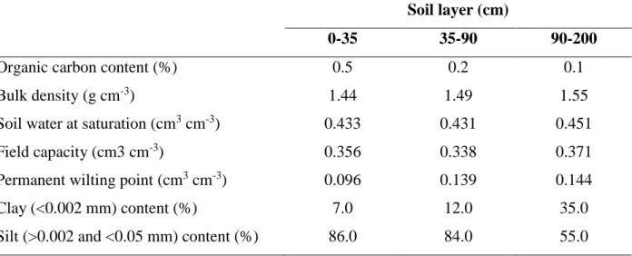
a depth of 90 cm to a depth of 200 cm. The data provided by Yang et al., (2006) on soil water content 185
at saturation, field capacity and wilting point for each layer were used as default values to estimate 186
the Campbell equation parameters (Table 2). 187
<INSERT TABLE 2 HERE> 188
Sensitivity analysis
189
The structure of the Daisy model is complex, including many simulated processes and potentially 190
many interactions; thus no a priori assumption can be made about the linearity or additivity of the 191
model response to parameter changes. Therefore, commonly applied one-parameter-at-a-time SA is 192
considered inappropriate (Saltelli & Annoni, 2010). In the present study, the sensitivity method 193
proposed by Morris, (1991) was adopted. The Morris method is considered a screening method that 194
provides a good compromise between efficiency and accuracy and it is particularly well-suited for 195
computationally costly models and/or when a high number of input parameters are considered (Xu & 196
Mynett, 2006; Campolongo et al., 2007). It has the advantage of being computationally less 197
demanding compared to the variance-based SA. By using a relatively small number of model
198
evaluations, a subset of influential and non-influential input parameters in a model could be identified. 199
The Morris method is based on the calculation of the so-called Elementary Effects (EE) of each input 200
parameter on model outputs. The EE method can be conceptualised as a randomised OAT design, in 201
which only one input parameter is modified between two successive runs of the model. This design 202
can be regarded as a global design covering the entire space over which the parameters may vary 203
(Wang et al., 2006). For a given parameter set 𝑋 = {𝑥1, ⋯ , 𝑥𝑛}, the elementary effect, 𝐸𝐸𝑌 (𝑥𝑖), of the 204
parameter, xi, on the output, y, is defined as follows:
205
𝐸𝐸𝑌 (𝑥𝑖) =𝑌(𝑥1,⋯,𝑥𝑖−1,𝑥𝑖+∆𝑖,𝑥𝑖+1,⋯,𝑥𝑛)−𝑌(𝑥1,⋯,𝑥𝑛 )
∆𝑖 (1)
206
where Y(x) is the output variable, 𝑥𝑖 is ith model input parameter, n is number of parameters, and ∆𝑖 207
8
methods, the perturbation Δ as defined by Morris, (1991) is a predetermined multiple of 1
𝑝−1 in which 209
p corresponds to the number of intervals/levels that a parameter range is divided by. Saltelli et al., 210
(2004) suggested the use of ∆ = 𝑝
2(𝑝−1) with the number of levels p ranging between 4 and 10. In this 211
work, the level p was fixed to 10 according to Zhan et al., (2013). 212
The whole procedure is repeated r times (r is the number of trajectories), providing r elementary 213
effects for each parameter where r typically varies between 10 and 50 (Campolongo et al., 2007). The 214
total number of model evaluations is then given by r(n+1). For this study, r = 50 was used and 215
considered adequate given the complexity of the DAISY model. Moreover, to prevent poor coverage 216
of the parameter space, the space-filling-design, introduced by Campolongo et al., (2007) was used 217
to assure a better spread of the points over the parameter space. This was achieved by first generating 218
1000 different trajectories and then selecting the r = 50 trajectories with the largest distance between 219
couples of trajectories over the parameter space. More details of the method are given in Campolongo 220
et al., (2007). 221
Because the units of the EEs are the units of the model output over the units of the parameter 222
increment, they cannot be readily compared to each other. We, therefore, used a scaled dimensionless 223
elementary effect as was defined by Sin & Gernaey, (2009) and which was also used inter alia by 224
Ruano et al., (2012): 225
𝑆𝐸𝐸𝑌 (𝑥𝑖) = 𝐸𝐸𝑌 (𝑥𝑖) 𝜎𝑥𝑖
𝜎𝑌 (2)
226
where 𝜎𝑌 and 𝜎𝑥𝑖 are the standard deviations of output Y and inputs xi, respectively.
227
The mean μ and standard deviation σ from the obtained SEEs are used to assess the importance of an 228
input parameter. A parameter with high overall importance on the output will have a high μ while a 229
parameter with a nonlinear effect or interacting with other parameters will have a high σ. To avoid 230
the cancelling of positive and negative effects on the mean, Campolongo et al., (2007) suggested the 231
use of the mean of the absolute values of the elementary effects (𝜇∗) instead of the mean: 232
𝜇𝑖∗ = ∑𝑟𝑖=1|𝑆𝐸𝐸𝑖|
𝑟 (3)
233
To decide whether a given parameter is influential or non-influential, the Morris sensitivity distance, 234
defined as the Euclidian distance 𝜖𝑖 = √𝜇𝑖∗2+ 𝜎
𝑖2 of (𝜇𝑖∗, 𝜎𝑖) from the origin (0,0), was used. A high 235
value of 𝜖𝑖 (> 0.1) indicates a relevant effect of the related ith parameter on the model output hence, 236
9
value was used. The parameters tested were further ranked according to 𝜖 values in order of 238
importance. The threshold value of 0.1 was also employed for the scaled 𝜇∗ by Cosenza et al., (2013). 239
The aforementioned sensitivity index (𝜖) was also used in other modelling applications (Xu & Mynett, 240
2006; Ciric et al., 2012; Pappas et al., 2013; Ojeda et al., 2014). 241
Parameters considered for sensitivity analysis
242
DAISY contains a large number of inputs and model parameters. Ideally, all parameters should be 243
screened to determine their relative importance. However, this would result in a large number of 244
simulations making such a study impractical. Based on experience, only a few parameters account for
245
most of the variability of model outputs. Therefore, the sensitivity analysis was restricted to 39 crop 246
parameters which for two crops sum to 78 parameters (including parameters referring to, among other 247
things, phenology, assimilation and respiration characteristics, and partitioning of assimilates to plant 248
organs). Furthermore, the analysis was also restricted to 28 soil parameters that for the three soil 249
layers sum to 46 (including among other things soil hydraulic parameters, SOM and soil microbial 250
biomass turnover rates). The parameters were believed to be potentially relevant parameters 251
controlling most of the processes represented by DAISY, and they have been reported in different 252
studies aiming at the calibration of DAISY for different output variables and different locations with 253
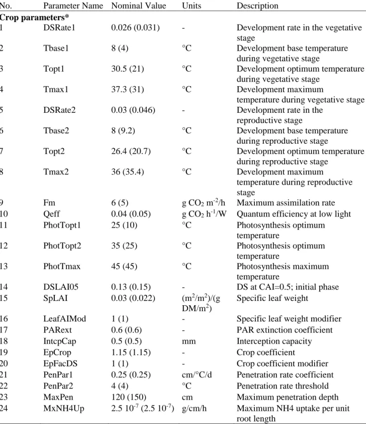
different climates, soils, crops and field management scenarios. The initial values of the selected crop 254
parameters were based partly on the values recommended for DAISY in the model crop library and 255
partly on literature screening and results from experimental studies at the Luancheng station. The 256
depth-dependent hydraulic parameters were provided by (Yang et al., 2006). The nominal values of 257
the cardinal temperatures (Tbase, Topt and Tmax) for vegetative and reproductive stages were 258
obtained for winter wheat and summer maize from Porter & Gawith, (1999) and Sánchez et al., 259
(2014), respectively. The default maximum rate of development DSRate1 and DSRate2 were adjusted 260
to be within the range of observed flowering and maturity dates, respectively, as recorded in the NCP. 261
Since there is not enough information about the prior probability distributions for each parameter, we 262
assumed an independent uniform distribution for each parameter. The bounds were set at 20% of 263
either side of a parameter nominal value as was also used by Xu & Mynett, (2006), Sourisseau et al., 264
(2008), Esmaeili et al., (2014) and more recently by Casadebaig et al., (2016). The groups of 265
parameters and the nominal values of all parameters are given in Table A1 (Annex A). The model 266
10
(ETa) and cumulated N leaching below the root zone during the cropping seasons of both crops. 268
Modelling procedure and statistical analysis
269
A total of 50*(128+1) = 6450 parameter sets were generated using the Morris method. The model is, 270
therefore, run for each parameter sets for the six cropping seasons simultaneously as winter wheat 271
and summer maize are grown in rotation (double cropping) in the NCP. This way the possible 272
contribution of the parameters of one crop on the model output of the following crop could be 273
investigated. This step is then repeated for each of the N fertiliser treatments. Finally, the model 274
selected outputs where extracted for each combination of crop × cropping season × N fertiliser 275
treatment and used to calculate the different Morris sensitivity measures. The outcomes of the 276
sensitivity analyses were then compared within each crop, to evaluate if and to which extent the 277
relative importance of crop and soil parameters varies (i) across the different seasons and (ii) among 278
the four fertiliser N treatments, and to evaluate the stability of the parameter sensitivity. This resulted 279
in 24 sensitivity analyses for each crop. 280
The effect of the different cropping seasons with different weather conditions and N fertilisation rates 281
on the number of influential parameters were tested using generalized linear models (GLM) for each 282
crop and output variable. In order to model these effects, all GLMs were carried out using Poisson 283
distribution with log link as we have count data (Zeileis et al., 2007). All GLM models were computed 284
using ‘glm’ function of R. Over-dispersion was investigated using ‘dispersiontest’ function of the 285
AER package (Kleiber & Zeileis, 2008) and was not found to be significant. 286
To measure the similarity between the parameter ranks resulting from different input combinations 287
(crop × fertiliser treatment × cropping season) and for each output variable, we used the top-down 288
coefficient of concordance (TDCC). This method was introduced by Iman & Conover, (1987) to test 289
the agreement between multiple rankings. The method emphasises the agreement between rankings 290
assigned to influential parameters and reduces the weight for disagreement between rankings assigned 291
to non-influential parameters (Helton et al., 2005; Confalonieri et al., 2010a). The Savage scores and 292
TDCC are calculated using Eq. 6 and 7, respectively. 293
𝑠𝑠(𝜖𝑖𝑗) = ∑ 1 𝑘 𝑛
𝑘=𝑅(𝜖𝑖𝑗) (6)
294
𝑇𝐷𝐶𝐶 =∑ [∑ 𝑠𝑠(𝜖𝑖𝑗) 𝑚
𝑗=1 ] 2
−𝑚2∙𝑛 𝑛
𝑖=1
𝑚2(𝑛−∑𝑛 1 𝑖⁄ 𝑖=1 )
11
where m designates the number of rankings to compare (in this study, m represents either the number 296
of seasons or the number of treatments N); 𝜖𝑖𝑗is the sensitivity index/measure for parameter pi (i =
297
1,…, n) and ranking j (j = 1,…, m), and 𝑅(𝜖𝑖𝑗) is the rank of 𝜖𝑖𝑗within ranking j. A rank of 1 is 298
assigned to the parameter pi with the largest value of 𝜖𝑖𝑗, a rank of 2 is assigned to the parameter with 299
the second largest value of 𝜖𝑖𝑗 and so on. In case of equal values of 𝜖𝑖𝑗, averaged ranks are assigned 300
to parameters. Values of TDCC close to one indicate a high level of concordance between compared 301
rankings, with agreement declining as TDCC decreases from one. Under the null hypothesis of zero 302
concordance between parameter rankings, the p-values for each TDCC can be calculated using the T 303
statistics (approximating a 2-distribution with n-1 degrees of freedom), derived from TDCC using 304
the following equation: 305
𝑇 = 𝑚 ∙ (𝑛 − 1) ∙ 𝑇𝐷𝐶𝐶 (8)
306
Additionally, the comparison regarding the similarity of classification into the most influential 307
parameters among contrasting weather conditions during the seasons 2003-04 and 2004-05 was 308
performed by analysing Venn diagrams. To further endorse the differences across seasons, we 309
performed a Multi-Dimensional Scaling (MDS) analysis (Hout et al., 2013), which allows 310
representing the distance among different rankings in a reduced number of dimensions. The 311
proximities among the Savage-score transformed ranks are computed using Euclidean distance for 312
each fertiliser treatment-season combination and presented in a two-dimensional plot as outlined by 313
Richter et al., (2010). 314
315
RDAISY toolbox
316
Several software packages enabling the automation of the SA of process-based models have been 317
developed and used to study the influence of model parameters on model outputs. In particular, the 318
‘Sensitivity’ package (Pujol et al., 2017) implemented in the open source software R includes 319
algorithms for global SA including the Morris, Sobol’ and FAST methods, among others. However, 320
using these methods with process-based models is not always straightforward and require that the 321
model is first coupled to the R platform in order to use one of the available functions of the 322
‘Sensitivity’ package. Therefore, a set of functions were created and wrapped into the RDAISY 323
toolbox to be able to operate the DAISY model through the R environment (Jabloun et al., 2014). 324
12
model calibration and model output visualisation by taking advantage of R’s extensive statistical, 326
mathematical, and visualisation packages. The RDAISY toolbox comprises three main functions, 327
update.InputFiles which update the DAISY input files given specified parameter values, runDaisy to 328
run the DAISY model from the R environment given the main DAISY setup file to run and 329
read.OutputFiles, which reads the generated output files with the possibility to restrict the columns 330
to read. These functions, even though written to operate DAISY from within the R environment, are 331
written in a way to be model independent. Therefore, it can be easily adapted to manipulate any model 332
that uses text files as inputs. The interactions between RDAISY toolbox and the DAISY model are 333
shown in Fig. 2. 334
<INSERT FIGURE 2 HERE> 335
336
The update.InputFiles function requires that a text template for each of the input files be created. 337
Each text template complies precisely with the format required by DAISY and contains markers 338
(unique parameter identifier/name) for all the parameters that need to be updated. These templates 339
can be created from the study case related input files by replacing each parameter value by its unique 340
text marker. Additionally, the update.InputFiles function requires that a data.table (Dowle et al., 341
2017) is created which stores the information about the parameter names to be updated, their default 342
values, the full path to the template file where the parameter is used as well as the full path to which 343
the newly updated input file will be saved to. An example of a template file for crop input file with 344
markers and their replacement by current values is shown in Fig. 3a and b respectively. 345
<INSERT FIGURE 3 HERE> 346
347
The runDaisy requires that the full path to the main setup file and daisy.exe is provided. The 348
read.OutputFiles is designed in a way to allow reading several output variables from different output 349
files at once. Therefore, a data.table with the full path to each of the output files to read and the names 350
of each output variable is required. For the function to work correctly it is crucial to set print_header
351
and print_dimension to false when specifying the output variables to log in DAISY (e.g. (output
352
("Soil Water Content" (when daily) (print_header false) (print_dimension false)))). The RDAISY 353
13
Results
355
Screening sensitive parameters
356
The results of the Morris analysis showed a linear relationship between µ* and σ, suggesting that 357
DAISY parameters with higher overall impacts had a higher nonlinear effect and/or interacted with 358
other parameters. The coefficient of determination (R2) considering all cropping seasons, N 359
treatments and model outputs ranged from 0.67 to 0.94 and from 0.77 to 0.96 for maize and winter 360
wheat, respectively. A subset of the results for the treatment N400 and the cropping season 2004-05 361
is shown in Fig. 4. 362
<INSERT FIGURE 4 HERE> 363
364
The number of sensitive parameters varied across cropping seasons and output variables and remained 365
relatively constant among N treatments. The number of influential parameters for each crop, model 366
output and for the seasons 2003-04 and 2004-05 and the N400 treatment is shown in Fig. 5. 367
Regardless of the cropping season, N leaching exhibited the highest number of influential parameters 368
for both crops (more than 38 parameters) and the number of parameters of major importance is 369
generally higher for hot and dry seasons (e.g. 2004-5, Fig. 5) as compared to average and wet seasons 370
(e.g. 2003-04). 371
<INSERT FIGURE 5 HERE> 372
373
In fact, the GLM models showed that cropping season characterised by different weather conditions 374
have a significant influence (p-value < 0.05) on the number of sensitive parameters (results not 375
shown). This observation was true for both crops and all model outputs except for N leaching for 376
which the number of influential parameter does not seem to be affected by weather conditions during 377
the investigated years. Besides, the N fertiliser rates have only a significant effect (p-value < 0.05) on 378
the number of influential parameters of the grain N content of both crops. The differences observed 379
between seasons was due to the model response to dry and wet conditions. In fact, when the dry 380
seasons 2004-05 and 2005-06 are excluded from the data used with the GLM models, the season 381
factor no longer have a significant effect on the number of sensitive parameters for both crops and all 382
model outputs. As for the N treatments, excluding the N200 treatment resulted in no significant effect 383
14
To compare the relative importance of the input parameters, the calculated Morris distances (𝜖) were 385
plotted against each input parameter for each response variable. Part of the results are reported in Fig. 386
6, where the parameter importance (in terms of 𝜖) obtained for winter wheat and maize is shown for 387
the N400 treatment over two cropping seasons 2003-04 and 2004-05. Parameters with 𝜖 below 0.1 388
were regarded as non-influential and were omitted from the figures. The season 2003-04 was chosen 389
as the one with optimal growing conditions, whereas the season 2004-05 was hot during summer and 390
dry during the wheat growing season (Table 1) and was therefore considered as dry and hot. 391
<INSERT FIGURE 6 HERE> 392
The Morris sensitivity analysis for the N400 treatment during the 2003-04 season revealed that 21 393
out of 39 crop parameters (54 %) and 28 out of 46 soil parameters (60 %) showed negligible effects 394
when all response variables were considered together. Low impact on model outputs was given inter 395
alia by parameters related to N concentration in the different plant parts (CrpNRoot, CrpNLeaf, 396
CrpNStem, CrpNOrg), maintenance respiration of the different plant parts (r_Root, r_Leaf, r_Stem, 397
r_SOrg), maximum NH4 and NO3 uptake per unit root length (MxNH4Up, MxNO3Up) and to a set
398
of parameters that govern crop phenology and crop photosynthesis (Tmax1, Tmax2, PhotTopt2, 399
PhotTmax). These parameters could be fixed at their nominal values without having a substantial 400
effect on model predictions. However, the sensitivity of the remaining parameters changed 401
substantially between the different response variables and their rankings differed between the two 402
crops (Fig. 6). For instance, while 13 crop parameters affected maize yield, we found 16 crop 403
parameters that affect wheat yield. When considering only those parameters having a significant 404
effect on all response variables, we found 11 influential crop parameters for wheat but only 6 for 405
maize, and 6 soil parameters were influential for wheat but none of them for maize (Fig. 7). 406
According to the Morris sensitivity distance (Fig. 6), the parameters related to crop phenology, crop 407
photosynthesis and assimilate partitioning were key parameters. In particular, maximum development 408
rate (DSRate1), the optimum temperature for growth (Topt1) and the quantum efficiency (Qeff) had 409
a high influence on all the output variables for both crops. Cumulated ETa over the cropping cycle 410
was also quite sensitive to the crop coefficient (EpCrop) and specific leaf area (SpLAI), particularly 411
for winter wheat. Interestingly, the results of the Morris analysis over the 2003-04 season suggest that 412
the parameters associated with the previous crop affected the cumulated N leaching of the following 413
crop. In the case of cumulated N leaching during the maize seasons, sensitive parameters were related 414
15
Similarly, N leaching and to a lesser extent grain N content over the winter wheat season were affected 416
by parameters related to maize. However, ETa, Yield and grain N content of maize were unaffected 417
by parameters relating to winter wheat. 418
<INSERT FIGURE 7 HERE> 419
420
Similar results were found for the soil parameters, and their importance also varied considerably 421
depending on the crop and the output variable considered. For instance, while maize yield was not 422
sensitive to any soil parameter, cumulated N leaching over the maize cropping season was highly 423
sensitive to water retention at field capacity (FC35 and FC90) and to the saturated hydraulic 424
conductivity (Ksat35 and Ksat90) of the topsoil (0-35 cm) and subsoil (35-90 cm) soil layer. On the 425
other hand, the output variables over the winter wheat cropping season were all sensitive to water 426
retention at field capacity and saturated hydraulic conductivity. Moreover, the soil organic matter 427
content (humus35) was a key parameter for both cumulated N leaching and grain N content of winter 428
wheat. 429
During the 2004-05 season, the results of the Morris method highlighted the importance of the 430
previous crop in affecting all the output variables of the following crop (Fig. 6). Besides the 431
parameters relating to crop phenology, crop photosynthesis and assimilate partitioning, the 432
parameters relating to root growth (PenPar1, PenPar2 and MaxPen) also had a substantial impact on 433
all outputs for both crops during this dry and hot season. Furthermore, it is remarkable that parameters 434
relating to the soil (i.e. hydraulic parameters) rank higher under limited water conditions for all model 435
outputs and both crops. In contrast to the wet season, 7 and 10 parameters relating to soil were shared 436
between the different outputs for maize and wheat, respectively (Fig. 7). 437
Morris SA excluding phenology-related parameters
438
Since most of the crop parameters considered in this analysis depend on crop phenology, the strong 439
sensitivity of DAISY to the parameterisation of crop phenology may mask the importance of other 440
parameters and processes. To investigate this, we repeated the SA with the crop phenology parameters 441
being excluded. Specifically, DSRate1, DSRate2 and cardinal temperatures (Tbase, Topt, Tmax) were 442
fixed to their pre-assessed values (Table A1, Annex A), and the Morris sensitivity indices were 443
16
of crop photosynthesis, assimilate partitioning, and root growth was further scrutinized, and their high 445
impact on model outcomes was also confirmed (results not shown). Most of the non-influential 446
parameters remain the same whether or not we considered the parameters related to phenology. 447
However, it is noteworthy that there are differences among the influential parameters, specifically the 448
parameters related to maize crop and influencing the output variables of the next wheat crop. We 449
found that the effect of the previous crop was more accentuated (i.e. higher overall ranks) when the 450
parameters related to phenology were included especially for crop yield. Overall, the effects of the 451
parameters relating to the previous crop and the differences between the sensitive parameters for wet 452
and dry years remained consistent and were not affected by fixing the parameters relating to crop 453
phenology. 454
Influence of weather conditions and crop management
455
The Morris SA was applied for each combination of crop × fertiliser treatment × cropping season, 456
which resulted in different Morris distance sensitivity indices. Fig. 8 depicts the variability over the 457
different cropping seasons of the Morris distance for winter wheat calculated for the N400 treatment. 458
In general, the Morris distance of the less influential parameters had low variability over seasons. 459
However, substantial variations in the Morris distance of the most influential parameters (with high 460
𝜖 values) driven by the variations in weather over seasons could be observed (Fig. 8), which might 461
result in different rankings over the different seasons (Fig. 9). The parameters DSRate1, DSRate2, 462
Topt1 and EpCrop presented the highest variability over seasons. These findings apply to all model 463
outputs. Similar results were also found for the other treatments. However, the results (not shown) 464
also revealed that the considered N treatments had no noticeable impact on the parameter ranking for 465
the considered output variables. In fact, the TDCC values obtained for the six cropping seasons from 466
the comparisons between parameter rankings obtained across fertilizer treatments were greater than 467
0.95 for both crops and for all output variables and years. 468
<INSERT FIGURE 8 HERE> 469
<INSERT FIGURE 9 HERE> 470
471
The TDCC coefficients were calculated for each output variable to provide a quantitative measure of 472
the concordance of the parameter rankings of the different combinations crop × fertiliser treatment × 473
17
values for each output. Summarized TDCC values are given in Table 3, where the TDCC values for 475
each output variable are displayed for each combination. The corresponding p-values are not reported 476
but were all 0.05. We obtained a different behaviour for different outputs. TDCC values were higher 477
than 0.92 for the N leaching output for both crops and around 0.9 for grain N content of winter wheat 478
suggesting that the rankings of important parameters remained relatively stable over seasons. 479
However, TDCC values were less than 0.9 for the rest of the output variables for both crops, which 480
implies that the ranks were different across years as was highlighted above. 481
<INSERT TABLE 3 HERE> 482
483
Fig. 10 shows the MDS plots obtained for grain yield for summer maize and winter wheat. The years, 484
which stand apart from the other years, in such a plot are considered with different parameter ranks. 485
From Fig. 10, it is clear that clusters around the season 2004-05 and 2005-06 (qualified as dry seasons) 486
and the rest of the seasons (qualified as wet seasons) were obtained for winter wheat when yield is 487
considered. Additionally, there is a cluster around season 2002-2003 for maize yield, which was also 488
a wet season. Generally, there were more explicit clusters around the different seasons for winter 489
wheat than for summer maize. The same observations were also obtained for ETa and to a lesser 490
extent for grain N output for both crops. No clear pattern was observed for N leaching for both crops, 491
which is in accordance with the TDCC values. We conclude from this that the low TDCC values and 492
the lack of similarity between the sensitive parameter ranks among years might be mostly due to the 493
differences between parameter ranks for wet and dry years. 494
<INSERT FIGURE 10 HERE> 495
Discussion
496
It is worth mentioning that the Morris method is traditionally used for parameter screening with a 497
very low number of sampled points. Based on the findings of Ciric et al., (2012), Zhan et al., (2013) 498
and Vanuytrecht et al., (2014) a small sample size would not be adequate to obtain a stabilised Morris 499
sensitivity distance for a complex model such as DAISY thus the high trajectory number (r = 50) used 500
in this study. This choice can be further justified by the nonlinear behaviour depicted by the high 𝜎 501
values (Fig. 4). We further acknowledge the subjectivity in the choice of the parameter ranges which 502
18
screening, narrowing or broadening the range of the parameter values could significantly influence 504
the parameter sensitivity as was delineated by Shin et al., (2013) and Paleari & Confalonieri, (2016). 505
Shin et al., (2013) also highlighted the importance of using ranges yielding plausible parameter sets, 506
which was believed to be the case for the ±20% used in this study. Therefore, we believe the results 507
of this SA were not biased by implausible model realizations. However, it should be stressed that 508
more work is needed to assist in the determination of parameter uncertainty ranges. 509
It is also important to recognise that the results of this SA were conditional on the cut-off used to 510
select the most sensitive parameters. Interestingly, using a different measure 𝛽𝑖 = 𝜖𝑖
𝜎 (σ is the standard 511
deviation of 𝜖𝑖 of all parameters) instead of using 𝜖𝑖 and a threshold of 0.85 to separate the most 512
important parameters from the less-important ones as was suggested by Lu et al., (2013) we found 513
the same set of most influential parameters for each combination crop × fertiliser treatment × season 514
× model output. These findings put more confidence on the parameters classified as most influential 515
for winter wheat and maize investigated in this study. 516
Model-dependent parameter sensitivity
517
Our analysis showed that for the N400 treatment, among the 124 parameters tested, only 34 and 36 518
common parameters were identified as being influential (𝜖 > 0.1) for the different model outputs 519
during season 2003-04 and 2004-05, respectively. This applied to both crops. A similar high number 520
of sensitive parameters was also found for other models. For instance, Hjelkrem et al., (2017) in a 521
recent study found that the BASGRA model was sensitive to a relatively large number of parameters 522
(45 parameters). Similarly, Casadebaig et al., (2016) identified 42 parameters to substantially affect 523
wheat yield in different tested environments in Australia using the APSIM-wheat model, and Specka 524
et al., (2015) identified a subset of 28 relevant model parameters from a set of 117 analysed 525
parameters for the agro-ecosystem model MONICA applied to different crops in Germany. It is 526
noteworthy that the same sensitive parameters, albeit differently ranked, were found for both crops 527
when all model outputs were considered. However, when model outputs were analysed separately, 528
the sensitive parameters and their number varied substantially with N leaching having the highest 529
number of sensitive parameters for both crops. Regardless of crop and season, N leaching was always 530
controlled by parameters relating to crop and soil; however, the other model outputs had the number 531
of their influential parameters differentiated by season whether it is a wet or dry season as was 532
19
reflects on the complex processes (i.e. the integrated effect of the redistribution of soil water and 534
subsequent convection-dispersion of nitrate) driving the N leaching (Manevski et al., 2016). It is 535
interesting to notice that some parameters, specifically soil related parameters, are shown to be 536
significantly more sensitive when evaluated in water-limited conditions especially for yield and grain 537
N. Thus, the sensitive (and non-sensitive) parameters cannot be assumed to be consistent across 538
seasons. These findings were confirmed for the different N treatments investigated in our study which 539
corroborates the findings of van Werkhoven et al., (2008) who demonstrated that when sensitivity 540
analyses are applied for watersheds spanning a hydroclimatic gradient, the most sensitive model 541
parameters might vary significantly across watersheds. 542
Similarly, Song et al., (2013) found that as the climate scenarios changed from wet to warmer and 543
drier conditions, the overall sensitivities of some parameters increased. In a recent study, Casadebaig 544
et al., (2016) found that the impacts of the influential parameters were strongly dependent on 545
environmental and management conditions. However, Tan et al., (2016) found that the weather 546
conditions had negligible effects on the identification of influential parameters of the ORYZA model 547
and that they only had slight effects on the ranks of the parameters' sensitivity for outputs in the 548
panicle-formation phase and the grain-filling phase of rice grown in China. The effect of dry and wet 549
years observed in our study might also be confounded with the effect of irrigation management since 550
irrigation amounts varied across seasons (Table 1). It should be noted, however, that the seasons 551
2004-05 and 2005-06, which are relatively hot and dry with a high cumulative ETo of 875 and 863 552
mm, respectively, showed relatively similar tendencies of parameter sensitivities (results not shown) 553
despite the difference in irrigation amounts for the two seasons (Table 1). Thus, the combined effect 554
of seasons and irrigation management would be worthy of further study. 555
Generally, the DAISY output responses were strongly influenced by the parameters related to crop 556
phenology, corroborating the findings of Krӧbel et al., (2010) and Manevski et al., (2016) who also 557
conducted a local SA on key parameters of the DAISY model for winter wheat and summer maize in 558
the NCP. We speculate that this is because many of the parameters in DAISY are formulated to 559
depend on crop phenology (Hansen et al., 2012). 560
The model behaviour proved to be highly consistent with the nature of the different processes that it 561
integrates. For instance, simulations of grain yield were influenced by the parameters related to crop 562
photosynthesis and to assimilate partitioning. Besides, simulations of crop evapotranspiration were 563
20
the one hand, and by other parameters linked with the responses of plants to light (Qeff) and 565
temperature (Topt1) on the other hand. In fact, a lower FC value means that the soil water holding 566
capacity is very low and thus a smaller amount of water is available for evapotranspiration and vice 567
versa (Abebe et al., 2010). These results are in concordance with the findings of Salazar et al., (2013) 568
who showed that the soil water balance simulated by DAISY was most sensitive to the potential 569
evapotranspiration and soil hydraulic parameters included in the Campbell model. Similarly, Esmaeili 570
et al., (2014), who conducted a global sensitivity analysis on the RZWQM model, found that the field 571
capacity in the upper 30 cm of the soil horizon had the most significant contribution (>30%) to 572
evapotranspiration uncertainty. The high sensitivity to the EpCrop parameter in all N treatments and 573
especially during dry and hot years reflects the role of evapotranspiration as a process of direct loss 574
of water from the soil-plant system, which has a considerable impact on the water balance 575
components of the winter wheat-summer maize double cropping system. Similarly, EpCrop and top 576
and sub-soil hydraulic properties were identified as sensitive parameters in simulating N leaching for 577
both crops, because these parameters directly affect soil water movement and the root water 578
uptake.The root water uptake also depends on the rooting depth and the root density distribution, as 579
well as on the soil water status in the rooting depth which was also depicted by the SA. In fact, the 580
parameters related to the root penetration rate (PenPar1) and root maximum penetration depth 581
(MaxPen) were identified as sensitive parameters in simulating ETa, N leaching, grain yield and grain 582
N content of winter wheat under water shortage conditions. 583
The absence of influence of parameters affecting N uptake (e.g., parameters related to N concentration 584
in the different plant parts) on simulated crop yield and N content indicate that N was not limiting 585
crop growth with current management setup. These results agree with the findings of Hu et al., (2006) 586
who, using the same dataset, found no statistically significant difference in grain yield and grain N 587
content between the different N treatments, implying no N shortage for the investigated N treatments. 588
It could also explain the strong rank concordance between the different fertiliser treatments. A 589
potential explanation of the similarities between N treatments is the issue of over-fertilisation. In fact, 590
a recent investigation by Ju et al., (2009) shows that the fertilisation rate in the NCP exceeds crop 591
requirements for maximum grain yield. In reality, the results of the SA might have been different if 592
there had been a zero N treatment. In fact, Zhao et al., (2014) found that N input with two fertilisation 593
rates (0 and 100 kg N ha−1) influenced the rank order of parameter sensitivities of the APSIM model. 594
It is noteworthy that N leaching depended mainly on the soil hydraulic parameters of the three soil 595
21
humus content and C/N ratio of the surface soil layer (0-35 cm) as well as the leaf photosynthetic 597
capacity (Fm) and photosynthetic quantum efficiency (QEff), were among the influential parameters. 598
This corroborates the findings of Manevski et al., (2016) who found, based on a sensitivity analysis 599
applied to 10 parameters of the DAISY model setup for the NCP, that a 10% change in humus content 600
and C/N ratio affected simulated nitrate leaching. They also found that nitrate leaching was strongly 601
affected by parameters governing crop vegetative development and growth (DSRate1 and Qeff). 602
Based on the Morris results, parameters associated with the previous crop showed major effect on 603
cumulated N leaching for the following crop and this was true for winter wheat and summer maize 604
regardless of the weather conditions. Besides, parameters relating to the previous crop also showed 605
major effect on crop yield, grain N content and cumulative ETa of the following crop only under dry 606
conditions (e.g. 2004-05 season). We speculate that the effect of the previous crop is driven by the 607
soil status (i.e. soil water content, organic matter and soil nutrients) left after crop harvest and before 608
sowing of the following crop, This has generally been referred to as the carry-over effects (Kollas et 609
al., 2015) such as N mineralising from the harvest residues of the previous year or altered soil water 610
content due to crop water uptake by the previous crop which was mainly the case in our study. For 611
instance, Li et al. (2007) showed that soil moisture before sowing of summer maize in the NCP is a 612
crucial factor that determines seedling growth, yield, and water use. 613
Practical implications for model calibration
614
Parameterization and identification of reliable estimates of the different parameters are a crucial issue 615
in modelling. Sensitivity analysis identifies the parameters that deserve more attention (Ma et al., 616
2012; Hjelkrem et al., 2017). The high 𝜎 values associated with the most relevant parameters (Fig. 4) 617
indicated a high degree of parameter non-linearity/interactions. Moreover, our findings showed that 618
there are multiple influential parameters for a single output variable that was considered sensitive for 619
multiple other processes (Fig. 4). This might substantially increase the frustration and subjectivity 620
that often characterize manual calibrations with increasing risk of calibrating parameters with 621
compensating effects. We therefore argue that the multi-objective calibration estimating all 622
parameters related to all output variables at once might be the best approach in this case. 623
Our analysis showed that about 34 parameters greatly influenced the outputs of the DAISY model for 624
both crops in the NCP. It is a valuable indication for the DAISY model users who may opt for 625
22
calibrating the parameters that have the most substantial impact on winter wheat and summer maize 627
grown in the NCP. Because of high N fertiliser rates in the NCP, the N treatments did not affect 628
parameter rankings. Therefore the calibration of the DAISY model in Luancheng could be limited 629
under these conditions to only one treatment. Consequently, the remaining treatments could be used 630
to validate the calibrated model. This approach was adopted by Hu et al., (2006) who used crop and 631
soil data of the same field experiment with N fertiliser at 200 kg N ha-1 yr-1 (N200) for the calibration 632
of the RZWQM model, which was subsequently evaluated using the other N treatments. 633
Moreover, our results suggest that the parameter rankings may differ between cropping seasons 634
depending on whether the cropping season is dry or wet. Specifically, the parameters relating to the 635
soil are more sensitive to seasons than other parameters, and significant uncertainty might be 636
introduced if the calibration is based only on wet years or dry years and the parameters are transferred 637
thereafter to conditions different from the calibration period. These findings support the idea that both 638
wet and dry periods should be included in the calibration and validation periods which was also 639
supported by Gan et al., (1997) and Arnold et al., (2012). Similarly, Li et al., (2012) stressed that a 640
sufficiently long period of records for model calibration should be used to ensure proper 641
representation of climate variability and to achieve stable model parameters. Furthermore, Bastola et 642
al., (2011) and Li et al., (2012) recommended that if model parameters are calibrated against a long 643
time series of historical data containing both wet and dry periods then these parameters can be 644
assumed to be valid also under future climates, with a higher degree of confidence. Moriasi et al., 645
(2016) also stressed that it is very important to ensure that the calibration period captures dry, average 646
and wet years to ensure that parameter values obtained are representative of the study area climate. 647
Our SA results further imply the importance of including different irrigation and/or nitrogen 648
treatments in the calibration process to have more representative parameter sets. 649
Another insight from our analysis is that parameters related to the previous crop could affect some of 650
the model outputs of the following crop, suggesting the need to consider the continuous crop rotation 651
when calibrating the most relevant parameters of both winter wheat and summer maize, especially 652
when calibrating ETa and/or N leaching. This is in line with the Teixeira et al., (2015) and Kollas et 653
al., (2015) who recently demonstrated the advantage of simulating continuous crop rotations 654
compared to single crops and years in New Zealand, particularly under limited growing conditions as 655
the carry-over effects could affect the growth of the next crop to some degree. 656
23
sensitive parameters. This signifies that it would be necessary to examine to which extent the 658
performance of the DAISY model will be affected with respect to reduction in the number of 659
influential parameters. 660
Conclusions
661
The dependence of process-based models on input parameters makes it particularly important to 662
understand their effects on model response outputs. The Morris screening analysis used in this study 663
helped identify the parameters with the greatest impact on the simulated grain yield, grain N content, 664
cumulated ETa and cumulated N leaching below the root zone of winter wheat and summer maize. 665
Our application of the Morris method to DAISY successfully tracked changes in sensitivities of the 666
most influential parameters with model outputs. The sensitivities of most parameters changed 667
substantially with cropping season, which represented different weather conditions. We also explored 668
the influence of N fertiliser rates on parameter sensitivities. 669
Out of 128 parameters, the Morris method identified 34 parameters to be most influential for the 670
simulation of investigated model output. These parameters mainly cover processes associated to crop 671
phenology, crop photosynthesis, assimilate partitioning, and root growth. The parameters associated 672
to soil hydraulics had major effect on winter wheat outputs and exhibits considerable influence on 673
the cumulative N leaching simulations and the water balance through their effects on the cumulative 674
ETa, as well as on the simulation of crop yield. Their effect on maize yield and grain N content, 675
however, was only apparent under hot and dry conditions suggesting that greater attention should be 676
paid to soil hydraulic parameters when the model is evaluated under dry weather and/or deficit water 677
conditions. The remaining 94 parameters only showed minor sensitivity. The large number of 678
parameters of minor importance indicates that the DAISY model could be simplified. 679
The parameterisation of the previous crop was shown to substantially affect cumulative N leaching 680
of the following crop as well as crop yield and grain N content depending on whether the cropping 681
season is dry or wet suggesting the importance of considering crop rotations especially when N 682
leaching is the target output. Ranking and relevance of most influential parameters hence depended 683
on weather conditions. Conversely, parameter rankings were shown to be consistent across N input 684
treatments when the amounts of N exceeds crop requirements for maximum grain yield. 685
The SA presented here has provided a deeper insight into how those sensitivities change depending 686
24
Morris method has considerably improved the understanding of the complex DAISY model and 688
enabled an extensive insight into the model response under limited conditions in the NCP. 689
Furthermore, the obtained results will considerably accelerate the calibration process of the DAISY 690
model when used in the NCP. Nevertheless, it should be noted that the most sensitive parameters 691
highlighted in this study might differ substantially if the model is used in different soil and weather 692
conditions. However, we believe that the developed RDAISY toolbox will serve as a basis for 693
following sensitivity analysis of DAISY. The primary functions developed for RDAISY are not 694
limited to the DAISY model, besides they could be readily applied to process-based models that 695
consider text files as inputs. These functions can also serve as a basis to implement automatic 696
calibration for the DAISY model by taking advantage of R’s extensive optimisation packages. 697
698 699
Acknowledgements
700
This study was financially supported by Aarhus University and by the Sino-Danish Centre for 701
Education and Research. It was further linked to the CRES Centre funded by the Danish Council for 702
Strategic Research under contract no: DSF-EnMi 09-066868 and partly supported by the National 703
Science Foundation of China (Project Nos. 41571088, 3171101264 and 41571493). 704
References
705
Abebe, N.A., Ogden, F.L. & Pradhan, N.R. 2010. Sensitivity and uncertainty analysis of the 706
conceptual HBV rainfall-runoff model: Implications for parameter estimation. Journal of
707
hydrology389, 301–310. 708
709
Arnold, J., Moriasi, D., Gassman, P., Abbaspour, K., White, M., Srinivasan, R., Santhi, C., Harmel, 710
R., Van Griensven, A., Van Liew, M. & others. 2012. SWAT: Model use, calibration, and 711
validation. Transactions of the ASABE55, 1491–1508. 712
713
Bastola, S., Murphy, C. & Sweeney, J. 2011. The role of hydrological modelling uncertainties in 714
climate change impact assessments of Irish river catchments. Advances in Water Resources34, 715
562–576. 716
717
Borgonovo, E. & Plischke, E. 2016. Sensitivity analysis: a review of recent advances. European
718
Journal of Operational Research248, 869–887. 719