INFERENCE FOR LARGE TREE-STRUCTURED DATA
KARTHIK BHARATH, PRABHANJAN KAMBADUR, DIPAK. K. DEY, AND VEERABHADRAN BALADANDAYUTHAPANI
Abstract. We develop a parametric inferential framework for fully observed tree-structured data containing a large number of vertices using the distributional properties of the Continuum Random Tree (CRT) introduced by Aldous [1993]. Under a hypothesis testing context, we develop tests based on two equivalent characterizations of the CRT. In both cases, the Rayleigh distribution with a scale parameter belonging to the exponential family arises as a limiting distribution and consequently, the test statistics enjoy optimal statistical properties. We examine properties of the parametric families of distribution induced through the two approaches and perform detailed simulations evaluating the performance of the proposed tests. A secondary contribution is in the efficient simulation of large trees of a particular class used in this article, which is of independent interest.
Keywords: Conditioned Galton-Watson trees; Dyck path; Brownian excursion; Distinguishability of parametric families; Rayleigh distribution.
1. Introduction
The statistical analysis of tree-structured objects has received appreciable attention in recent years owing to the emergence of datasets wherein the underlying quantities of interest allow for tree-like representations. However, some central challenges have stymied the systematic development of tools for statistical inference: The non-Euclidean nature of the underlying space offers considerable challenges while developing probability models for fully observed trees; tree-structured data rarely contain the same number of vertices leading to issues in comparing trees of differing sizes; generating trees from a probability model for simulation purposes is not straightforward. Motivated by these issues, our approach in this article is based on the abstract notion of a Continuum Random Tree (CRT) from Aldous [1991a] and Aldous [1993] which arises as a continuous limit as the number of vertices grows without bound for a large class of random trees. Our objective is to investigate the utility in employing the CRT in developing asymptotic inferential tools on fully observed tree-structured data containing a large number of vertices. To this end, we confine our attention to finite, rooted trees: trees with a distinct vertex, referred to as the root, containing a finite number of vertices. These trees can be labelled or unlabelled, ordered or unordered, have positive branch lengths, unequal number of vertices and are referred to in combinatorial literature as simply generated trees, or equivalently (leaving aside
some extreme cases) within the probability community asConditioned Galton-Watson trees (CGW)
obtained as the family tree of a Galton-Watson process conditioned on a given total number of vertices. The CRT is an archetypal example of the weak convergence paradigm proposed by Aldous [1994b]
based on an isometric`1 embedding of a tree with n vertices such that the graph distance between
vertices are preserved. Such an embedding makes possible comparing trees for differentn. Equipped
with a probability measure on the vertices, a continuous weak limit asntends to infinity is determined
which then offers insight into structural and numerical properties of the original object which would otherwise be hard to ascertain. We propose to embed the statistical problem of interest on large trees in the continuous environment offered by the CRT and develop tools based on the two equivalent characterizations of the CRT leading to the definition of simple parametric probability models on trees. The distribution of the CRT can be specified in four equivalent ways of which the following two will be of primary concern in this article (see Aldous [1991a] and Aldous [1993]): as a weak limit of family trees of critical Conditioned Galton-Watson processes; distributions of spanning subtrees which are analogous to finite dimensional distributions of a stochastic process. The first specification
is characterized by a continuous function on the vertex set, referred to as aDyck path, obtained from the depth-first walk at unit speed on the tree which converges to a Brownian excursion. The second specification is based on the limiting distribution of family of subtrees referred to as Least Common Ancestor trees. These considerations on CGW tree-models for tree-structured data lead us to the primary focus of this article:
(i) Developing parametric families using the limiting distribution of a special class of subtrees of the CRT for hypothesis testing;
(ii) Using the Dyck path representation to define parametric families for hypothesis testing based on the Brownian excursion approximation;
(iii) Efficient simulation of CGW trees.
The parameter of interest is the variance of the offspring distribution generating the CGW trees. The parametric setup allows us to rigorously examine the theoretical properties of the family of distributions on trees and the proposed tests using conventional ideas such as Neyman-Pearson tests, UMP tests, exponential family etc. It will be seen that the induced family in (i) and (ii) is the Rayleigh family parameterized by a scale factor given by the variance of the offspring distribution of the CGW tree; the Rayleigh with a scale parameter is a member of the one-parameter exponential family enjoying various desirable statistical properties. While we restrict our attention to hypothesis tests, this article ought to be viewed a first step of a systematic program in developing statistical procedures on large trees using the CRT.
Another contribution of this article is in the efficient simulation of critical CGW trees which encom-pass a broad class of random trees including Catalan trees, Cayley trees, Binary trees, uniform random trees etc. We use the efficient algorithm for generating CGW trees proposed by Devroye [2012] for our simulations which has a universal linear expected run-time. As a consequence, we are able to generate a large number of CGW trees with thousands of vertices fairly quickly under a parallel distributed computing setup. The generation of CGW trees is, in general, not a trivial matter, and with our software, we provide means to simulate a broad class of trees from a critical Galton-Watson process which can be used as “ground-truth” for simulation experiments involving tree-structured data.
Methodology on tree-structured data has hitherto been characterized by nonparametric or algo-rithmic approaches (Wang and Marron [2007], Busch et al. [2009], Aydin et al. [2011], Shen et al. [2013], Wang et al. [2012], Aydin et al. [2009], Rosa et al. [2012] etc.). In relation to our approach, Shen et al. [2013] used FDA methods on Dyck paths using an aligning mechanism which led to the creation of some spurious tree-structures—for eg. negative branch lengths—while exploring modes of variation in the trees in a regression problem. A parametric route was taken by Steele [1987] wherein a one-parameter exponential family of distributions on labeled trees was proposed with the natural parameter representing the expected number of leaves (terminal vertices) in the trees. In similar vein, but with phylogenetics in mind, Aldous [1996] proposed a beta-splitting parametric model for clado-grams; he noted the utility of a simple parametric model for phylogenetic tree construction. Motivated by the parametric approaches, we will consider a few one parameter family of distributions for testing statistical hypotheses on CGW trees considered in this article which are induced from the distributional properties of the CRT and Brownian excursion. CGW trees can be used as models for tree-structured data frequently encountered in many scientific settings. For instance, plane-rooted trees are considered in Busch et al. [2009] under the context of a protein classification problems; Shen et al. [2013], Aydin et al. [2009], Aylward and Bullitt [2002] modeled brain artery data as three dimensional trees embed-ded on the plane; also see Yang et al. [2005] and Tatikonda and Parthasarathy [2010] for datasets in the context of XML documents and secondary structure of RNA.
In section 2 we review the key ingredients of the CRT including CGW trees, Dyck paths and Least Common Ancestors trees. In section 3, we propose a parametric family induced by the spanning subtrees of the CRT, examine its properties, and propose one-sample and two-sample tests for distri-butions on trees. In section 4, we propose a parametric family based on the random projection of Dyck path representation and propose one and two-sample tests for distributions. In section 5, we generate CGW trees using the algorithm proposed by Devroye [2012] and verify the validity of the theoretical
results and performance of proposed tests. Section 6 discusses some salient aspects of our approach and comments on possible extensions. Proofs of results and details of simulations are relegated to the Appendix in section 7.
2. Preliminaries
2.1. Representation of trees. Consider a finite rooted treeτnas set of verticesV(τn) = (root, v1, . . . , vn−1)
and a set of edgesE(τn) = (e1, . . . , en−1) , represented as a point
τn=
V(τn),E(τn)
in the spaceTn×Rn+−1whereTnis the set of all finite trees onnvertices. One way to compare different
size trees is to embedτn = (V(τn),E(τn)) as an element of the linear space `1, the Banach space of
infinite sequencesx= (x1, x2, . . .) such that||x||=Pi|xi|<∞. Such an embedding makes possible
comparison and scaling of trees consisting of different number of vertices in a natural way. Formally,
suppose d(v1, v2) is the distance between two vertices defined as the sum of edge lengths along the
unique path fromv1tov2. The embedding ofτn= (V(τn),E(τn)) as a subset of`1is the determination
of pointswi for 1≤i≤nin `1 such that ||wi−wj||=d(vi, vj) for all 1≤i, j≤n. Then, the subset
of`1 containingw1, . . . , wn and the connecting paths is referred to as the set representation ofτn. In
this article, however, we shall not directly employ the set representation; the use of Aldous’ results obtained through the set representation, implies its indirect use. The formal definition the CRT is
based on the set representation S and a probability measure µ on `1 connected to S through two
technical conditions; see p. 253 in Aldous [1993]. The pair (S, µ) is then the CRT. We shall only be
concerned with the CRT through its distributional properties.
2.2. Conditioned Galton-Watson trees and random sampling. Given a probability distribution (πk, k= 0,1, . . .) on the non-negative integers, or equivalently a random variableξwith distributionπk,
we construct aGalton-Watson treeτ recursively starting with root and giving each node a number of
children that is an independent copy ofξ;P(ξ=k) =πk fork= 0,1, . . .is referred to as the offspring
distribution and the out-degrees of the vertices are i.i.d. copies of ξ from πk). As a consequence, ξ
induces a unique distribution onτ as
P(τ=t) = Y
v∈V(t)
πo(v,t),
whereo(v, t) is the out-degree or the number of children of vertexv in treet.
If one wishes to model a set of tree-structured data using Galton-Watson trees, two issues arise at this point: Galton-Watson trees, with positive probability, can be infinite, whereas observed trees in practice are always finite; secondly, how could we ensure that the observed trees have been collected
through random sampling? We shall address these issues by considering Conditioned Galton-Watson
(CGW) trees; these are Galton-Watson trees conditioned on total progeny. That is, the distribution
of a CGW treeτn conditioned to have nvertices is
P(τn=t)∝
Y
v∈V(t)
πo(v,t) on{t: cardinality ofV(t) =n}.
Importantly, it is known, that for a fixed offspring distributionπk, the corresponding CGW tree can be
viewed a being picked according to a uniform distribution on certain types of tree withnvertices. For
example, if we wish to choose a strictly binary tree (0 or two children only) withnvertices according
to a uniform distribution on the space ofn-vertex binary trees, then, we can equivalently construct
a CGW tree with a offspring distribution 0.5 each for 0 and 2 children. We enumerate a few useful
classes of trees for modeling purposes:
(i) Ordered trees with unrestricted degree: CGW trees with offspring distribution given by a
Geo-metric distribution with success probability 1/2;
(ii) Binary trees: CGW trees with vertices containing 0,1 or 2 children with a Binomial distribution with 2 trials and success probability 1/2;
(iii) Strict binary trees which are ordered: CGW trees with vertices containing either 0 or 2 children with equal probability 1/2;
(iv) Unary-binary trees which are ordered: CGW trees with vertices containing 0, 1 or 2 children each with probability 1/3;
(v) Unary-binary trees which are unordered and unlabelled: CGW trees with vertices containing 0, 1 or 2 with probabilitiesπ0=2+1√2,π1=
√ 2
2+√2 andπ3= 1
2+√2, respectively.
(vi) m-ary trees: CGW trees with vertices containing 0,1, . . . , mform >3 children with distribution
given by a Binomial withmtrials and success probability 1/m1.
Ordered trees imply that they can be embedded on the plane and therefore possess a natural labelling mechanism. From a tree perspective, this implies that there is an order amongst the children at any given vertex. Note that the offspring distributions of the CGW trees considered are with unit mean implying that the Galton-Watson process generating the tree is critical. This is because conditioning on
nmakes the family of offspring distributions parameterized by a mean parameter identically distributed
(see Kennedy [1975]). While it is conceivable that inference on such trees can be performed by a mere counting of the number of observed children at arbitrary, knowledge of distributions of local structural aspects like height, variations in branching structure and also information about branch lengths are not easy to obtain. In this article, we shall consider CGW trees and refer to them simply as trees.
2.3. Dyck paths. Any rooted ordered treeτn can be uniquely coded by a traversal of the tree; when
the traversal is a depth-first walk, one can construct a function which is a bijection to the tree in
the following manner: for ease of exposition, assume that the edges or branches of a treeτn withn
vertices have length 1. For a fixed positive integern, Dyck paths are lattice excursions of length 2n,
that is sequences (dj,0 ≤ j ≤ 2n) where d0 = d2n = 0 and dj > 0 with dj+1−dj ∈ {−1,+1} for
all 0≤j ≤2n−1. Imagine the motion of a particle that starts at timet = 0 from the root of the
tree and then explores the tree from the left to the right, moving continuously along the edges atunit
speed until all the edges have been explored and the particle has come back to the root. Since it is clear that each edge will be crossed twice in this evolution, the total time needed to explore the tree
is 2n. For simplicity, suppose all edges are of unit length, the value Hn(s) of a continuous function
Hn: [0,2n]→R≥0at times∈[0,2n] is the distance (on the tree) between the position of the particle
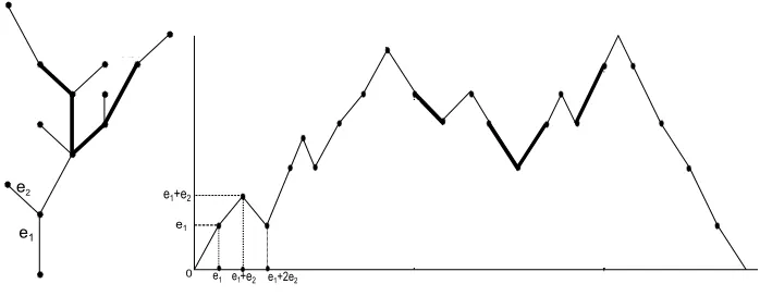
at timesand the root; figure 1, taken from Pitman [2006], offers a more intuitive description with edge
lengths not all equal to one. Therefore, ifτnis a tree of sizenthe sequence (Hn(0), Hn(1),· · ·, Hn(2n))
is its Dyck path of length 2n. The representation of the Dyck path of a treeτnin terms of the distance
dbetween its vertices is related to the functionHn as
(2.1) Hn(s) =d(root, v),
where v is the vertex obtained during the depth-first walk such that the sum of the edges traversed
tillv iss. This discussion is formalized by the following proposition whose proof is straightforward.
Proposition 1. The map τn 7→(Hn(0), Hn(1),· · · , Hn(2n)) is a bijection from the set of plane trees with sizento the set of all Dyck paths of length 2n.
The key result combining the two ideas is the following result in Aldous [1993]:
Theorem 1. Let τn be a CGW tree conditioned to have n vertices with offspring distribution with mean1 and variance σ2
∈(0,∞). Let Hn(k),0≤k≤2n be the Dyck path associated with τn. Then, asn→ ∞through the possible sizes of the unconditioned Galton-Watson tree,
1
√nHn([2nt]),0≤t≤1
⇒
2 σB
ex
t : 0≤t≤1
whereBex is the standard Brownian excursion and
⇒implies weak convergence of processes inC[0,1], the space of continuous functions on[0,1], and[·]stands for the integer function.
1There is an identifiability issue for them-ary trees with m= 3 since the variance is 2/3 which is the same as the variance for the unary-binary trees.
H(x)
H(y)
γ(x) γ(y)
e1 e2
e1
e1 e1+e2
+e2
[image:5.612.137.486.89.225.2]τ 0 e1 e1+2e2 2L(τ)
Figure 1. A tree with root at the bottom and its corresponding Dyck path. The
x axis ranges from 0 to twice the sum of lengths of the edges; the Dyck path is
constructed by traversing the tree in a depth-first manner at unit speed.
Roughly, the Brownian excursion in the limit is the ‘Dyck path’ of the CRT and the distribution of the CRT is specified by a careful construction from the excursion.
2.4. Least Common Ancestor subtrees. We define here the class of spanning subtrees which
characterize the distribution of the CRT. For a CGW finite treeτn = (V(τn),E(τn)), define its Least
Common Ancestor (LCA) tree in the following manner: choose a subset B of V(τn); for vertices v1
andv2in B find their last common ancestor, or the branch point after which the paths to thev1and
v2from the root diverge or branch out. Now, the LCA tree corresponding to the subsetB of vertices
of τn is the tree, denoted as LCA(τn, B), containing the root, the vertices of B and all the branch
points with distances from the root to the vertices ofB preserved. Figure 2 illustrates this idea with
B={v1, v2, v3, v4}; the branch points areb1 andb2, and in order to preserve the distances from root
to the vertices ofB, the new edge from the branch points to elements ofB are the sum of the edges
along the path from the root to elements ofBin the original tree. Now, for a treeτn randomly reorder
1
v
2
v
3
v
4
v
1
v
3
v
4
v
1
b b2
1
b
2
b
2
v
1
e
2
e
3
e
4
e
2 1 e
e e3e4
Figure 2. A tree on the left and its LCA tree on the right corresponding to vertices
{v1, v2, v3, v4}. The LCA tree contains the root, the branch pointsb1,b2 and the set
of vertices{v1, v2, v3, v4}.
the vertex setV(τn) to obtain (vn,1, . . . , vn,n). For a fixedk < n, consider the LCA tree ofτn defined
byLCA(τn,(vn,1, . . . , vk,n)); this is akin to pickingk < nvertices according to a uniform distribution
onV(τn). LCA trees have been used in the context of reconstruction of the trees; see Gronau and
Moran [2007] for a phylogenetic applications and Aho et al. [1981] for related work in a computational
context. Aldous showed that for eachk, asn→ ∞, the random LCA trees LCA(τn,(vn,1, . . . , vk,n))
converge, as subsets of`1, to a limit treeL(k), which is strictly binary (each vertex has either 0 or 2
[image:5.612.113.472.459.567.2]children) withkleaves or terminal vertices. The key point here is that Aldous proved that the family
(L(k), k ≥1) is a consistent class of subtrees which characterize the CRT (S, µ); in other words, for
modeling purposes one can justifiably view the class (L(k), k ≥1) as finite dimensional distributions
of the CRT. One can then use the distribution of the limiting class to approximate the distributions of the LCA trees of CGW trees.
2.5. A parametric family. Throughout, we shall assume that we have a random sample of
fully-observed treesτni = (V(τni,E(τni))) for i = 1, . . . , N from some distribution on the product space
⊗N
i=1Tni×R
ni−1
+ . The six types of CGW trees outlined in section 2.2 represent a very broad class for
modeling purposes. The variancesσ2 of the distributions considered are, respectively, 2,1
2,1, 2 3,
2 2+√2
and m−1
m for m = 4,5, . . .. Since the offspring distributions completely characterize the law on
the CGW trees, it is conceivable that a class of probability distributions on the non-negative
inte-gers parameterized by their variance parameter σ2 can be used for statistical purposes. Let
S = n
2,1 2,1,
2 3,
2 2+√2,
m−1
m ;m= 4,5, . . .
o
. Then, the class
(2.2) nπk,σ2 :k= 0,1,2, . . .;σ2∈ S
o
is a one-parameter class of probability models for fully observed finite rooted, ordered trees, with the constraintsP∞k=0kπk,σ2 = 1 andP∞k=0k2πk,σ2 <∞, and setσ2 =P∞k=0k2πk,σ2−P∞k=0kπk,σ2
2
. The first constraint implies that the Galton-Watson branching process generating the CGW tree is critical. An obvious shortcoming with the class in (2.2) is the absence of any branch-length information in the distribution—the probabilities purely reflect the topological structure or “shapes” of trees.
Since our primary interest is in developing hypothesis tests for parametric families, we recall the definition of distinguishable property of parametric families.
Definition 1. Suppose Θ is an index set and Θ0and Θ1are disjoint subsets of Θ such that Θ0∪Θ1= Θ.
Denote byH0 andH1the null and the alternative hypothesis that θis a member of either Θ0 or Θ1.
Then, the set of probability measuresnPθ:θ∈Θ
o
is distinguishable if
(i) Pθ6=Pθ0 for all distinctθ, θ0∈Θ;
(ii) There is at least one Borel set Asuch thatPθ(A)6=Pθ0(A) forθ∈H0 andθ0 ∈H1.
This is a crucial requirement while testing with parametric families; it will be shown that the parametric families induced by the LCA-tree based approach and Dyck path approach satisfy the above conditions.
3. Parametric family and test from LCA trees
In this section we consider a parametric family for finite rooted trees which may or may not be
ordered; the canonical CGW tree containsn vertices and methodology is developed by constructing
a subtree by choosingk < nvertices according to a uniform distribution on the vertex set excluding
the root; the root is always included in the subtree as its root. Recall that any treeτn is represented
as (V(τn),E(τn)) with vertex setV(τn) ={root, v1, . . . , vn−1} and edge set E(τn) ={e1, . . . , en−1}; a
similar representation holds for any subtree. From section 3, it is known that the family of subtrees
(L(k), k ≥ 1), arising as the limit of LCA trees, can be regarded as consistent “finite dimensional
projections” of the CRT. For a random CGW treeτn with distribution πσ2 for some σ2 in S,
con-sider its LCA(τn, v1, . . . , vk) defined earlier for k < n vertices chosen randomly from V(τn). Since LCA(τn, v1, . . . , vk) converges in distribution toL(k) (see p. 251 in Aldous [1993]), the limit
distribu-tion inheritsσ2too. Lemma 21 in Aldous [1993] provides the limit distribution and Theorem 3 proves
the characterization of the CRT by (L(k), k ≥1). We combine the two results into a single Lemma
for our purposes.
Lemma 1. There exists a consistent family (L(k), k ≥ 1) of strictly binary trees which define the CRT having the density
f(l(k)) = "k−1
Y
i=1
1 2i−1
#−1
1 2k−1se
−s2
2 ,
wheres=e1+· · ·+ek−1 andl(k) is a strict binary tree withkvertices.
We propose to use the density above for the LCA trees of large CGW treesτnwith the dependence
onσ2 introduced in a natural manner: 1/σ will be the scale parameter; as a consequence, we have a
parameterized class of distributions forLCA(τn, v1, . . . , vk), given by
(3.1) nfσ2:σ2∈ S
o
,
where, for the LCA tree withkverticeslk,
(3.2) fσ2(lk) =
"kY−1
i=1
1 2i−1
#−1
1 2k−1σ
2se−s22σ2,
wherelk has edge setE(lk) = (e1,· · · , ek−1). The vertex set manifests itself in the factor 2−(k−1); see
Aldous [1993] for details.
Remark 1. Note that the density in (3.2) uses information about the branch-length aspects of the tree;
this is in contrast to the distribution in (2.2). Choosing k vertices from n according to a uniform
distribution might appear to be restrictive. This can be relaxed in a simple manner as remarked in p.274 of Aldous [1993]. The word “consistent” in the Lemma refers to two properties: if an edge is
removed from L(k), then the remainder tree is distributed as L(k−1); second, the labeling of the
vertices are exchangeable. Upon ignoring the normalizing factors, when viewed as a density of the random variable representing the sum of the edges, the density in (3.2) is the Rayleigh density.
While class in (3.1) is a family of distributions on the LCA trees and consistent for the CRT, it is
not immediately clear if the class can be extended toτn for everyn; this is especially important while
developing tests based on the LCA trees. Specifically, noting the obvious fact thatLCA(τn,V(τn)) =
τn, it is necessary that fσ2(·) defined onLCA(τn, B) for anyB ⊂ V(τn) can be extended toτn upon
inserting vertices fromV(τn)−BtoLCA(τn, B), whileretaining the interpretability ofσ2. To formalize
this ideas, recall thatτn = (V(τn),E(τn)) resides inTn×Rn+−1; its LCA corresponding toB ⊂ V(τn),
where |B| = k, lies in Tk ×Rk+−1. Then, for all k and n with k < n, the class in (3.1) defined on
Tk×Rk+−1can be extended toTn×Rn+−1, or isn-extendable, iffσ2(·) onLCA(τn, B) can be recovered
by marginalization overfσ2(τn) onTn×R+n−1 for everyσ2. Denote byPσ2 the law on CGW treesτ
withσ2
∈ S corresponding to the density in (3.1). The following Propositions justifies the use of the
class in (3.1) for defining a proper family onτn for every n, and its amenability for testing purposes.
Proposition 2. The class nfσ2 :σ2∈ S
o
onTk×Rk+−1isn-extendable for everyn.
Proposition 3. The parametric class of probability measures nPσ2 :σ2∈ S
o
is distinguishable.
Remark 2. The issue of extendability was considered by Shalizi and Rinaldo [2013] in the context of
Exponential Random Graph Models, where they defined a notion of the class of distributions being projectivefor the exponential family of distributions. Without going into details of their work, it suffices
here to note that the density in (3.2), when viewed as the density ofs, is the Rayleigh distribution with
a scale factorσ, which belongs to the one-parameter exponential family. Then,s=e1+· · ·+ek−1is
the minimal sufficient statistic forσ2and is clearlyseparableas defined by Shalizi and Rinaldo [2013]—
adding an edge increases the value of the sufficient statistic by an amount equaling the edge length.
In fact, theconditional volume factor defined by them, in our case, is precisely the length, saye, of
the newly added edge when viewed as the Lebesgue measure of the interval [0, e] as a generalization of
the definition of conditional volume factor. We remark here that the sufficient statisticsinduces the
density on the tree and the density is hence with respect to the Lebesgue measure. This is in contrast to the density in the Exponential Random Graph Models which posses density with respect to the counting measure.
We now put to use the parametric class in (3.1) to the inferential problem of testing hypothesis on sets of random trees. The method involves choosing a subset of vertices (excluding the root) uniformly from the vertex set of each tree and constructing its corresponding LCA tree; this leads to a sample of LCA trees. The LCA trees are assumed to have been generated from the family in (3.1)
parameterized byσ2 as the number of vertices of the original trees approach infinity. The conclusions
of the subsequent hypothesis test on the LCA trees are extended on to the fully observed trees using Proposition 2.
Theorem 2. Suppose we have an independent sample of CGW trees τni = (V(τni,E(τni))) for
i = 1, . . . , N from a distribution πσ2 on the product space ⊗Ni=1Tni ×Rn+i−1 with σ2 ∈ S. Let K = (K1, . . . , KN), where Ki ⊂ V(τni) chosen according to a uniform distribution on V(τni) for
eachi= 1, . . . , N; let #Ki denote the cardinality of setKi and denote byCα,2N, the αth percentile of a Chi-square distribution with2N degrees of freedom.
(1) GivenK, define the critical function
φ(K, N, α, σ2 0) =
1 ifσ2
0
N
X
i=1
s2
i < Cα,2N
0 ifσ2
0
N
X
i=1
s2
i > Cα,2N,
wheresi=e1+· · ·+e#Ki−1. Then, conditional onK, for the pair of hypothesesH0:σ
2=σ2 0
vs H1 : σ2 = σ21 where σ21 > σ20, the test given by φ(K, N, α, σ20) is such that as ni → ∞ for each i = 1, . . . , N, Eπφ(K, N, α, σ20) → α, and is the most powerful test for the pair of
hypotheses.
(2) Given K, the likelihood ratio test for testing H0 : σ2 =σ20 vs H0 : σ2 6=σ20 is given by the
critical function
ψ(K, N, α, σ2 0) =
1 ifσ2
0
N
X
i=1
s2
i < Cα2,2N or σ20
N
X
i=1
s2
i > C1−α
2,2N;
0 otherwise,
where asni → ∞for eachi= 1, . . . , N,Eπψ(K, N, α, σ20)→αand all other quantities are as
in part 1.
Theorem 3. Suppose we have two independent samples of CGW trees τni = (V(τni),E(τni)) for
i= 1, . . . , N1, and ηmj = (V(ηmj),E(ηmj)) forj = 1, . . . , N2, from distributions πσ12 and πσ22 on the
product spaces ⊗N1
i=1Tni ×R
ni−1
+ and ⊗
N2
j=1Tmj ×R
mj−1
+ , respectively, with σ 2
i ∈ S for i = 1,2. Let
K = (K1, . . . , KN1), whereKi ⊂ V(τni) is chosen according to a uniform distribution on V(τni) for
i= 1, . . . , N1; in similar fashion letL = (L1, . . . , LN2), where Lj ⊂ V(ηmj) is chosen according to a
uniform distribution onV(ηmj). GivenKandL, asni, mj → ∞, for eachiandj, the likelihood ratio
test of asymptotic sizeα, for the pair of hypotheses H0:σ21=σ22 vsH0:σ126=σ22 is given by
φ(K,L, N1, N2, α) =
(
1 if N1PNi=12 r 2
i
N2PNi=11 s2i
< Fα
2,2N2,2N1 or
N1PNi=12 r 2
i
N2PNi=11 s2i
> F1−α
2,2N2,2N1;
0 otherwise,
wheresi =eτ1 +· · ·+eτ#Ki−1 and rj =e
η
1+· · ·+e
η
#Lj−1, for 1 ≤i≤N1 and 1 ≤j ≤N2, with e
τ
and eη representing generic elements of the edge sets
E(τ) and E(η) respectively; Fα,a,b denotes the αth percentile of anF distribution with a, bdegrees of freedom.
Remark 3. Observe that the tests in Theorem 2 and 3 are finite sample tests in the sense that we do
not let the sample sizeN1 or N2 tend to infinity. The class in (3.1) is a valid distributional class on
a set of trees and whenever the data generating model is a CGW model, the test represents a useful tool to distinguish between a fairly general class of trees. It is evident now how crucial Proposition 2 on extendability is for inferential purposes.
4. Parametric family and test based on Dyck Path
In the section, we consider a parametric class and develop tests for trees which are ordered and can be embedded on the plane. The pertinent question behind the Dyck path representation of an ordered tree
is this: suppose a CGW treeτnis distributed as a member of the class (2.2); what is the ramification of
the bijective transformationτn 7→Hn on the class{πk,σ2 :k= 0,1,2, . . .; 0< σ2<∞}? If we propose
to develop inferential tools on the space of Dyck paths, it is then required to establish the equivalence of statistical procedures, perhaps in the Le Cam sense, on{πk,σ2 :k= 0,1,2, . . .; 0< σ2<∞}and the
class resulting from the transformation. Indeed, this requires us to know exactly the induced class prior
to establishing equivalence. The probabilistic structure of the Dyck path corresponding to anarbitrary
CGW tree is not easily ascertained; only under the special case when the offspring distribution is the Geometric with success probability 1/2, is it known that the corresponding Dyck path can be modeled as a simple symmetric random walk conditioned on first return to 0 (see Aldous [1993]). This issue poses a serious difficulty if one wishes to establish some sort of equivalence between procedures on the two classes using the notion of a deficiency distance. However, weak equivalence of the procedure
is easily established as consequence of the invariance principle in Theorem 12: for a CGW treeτ
n, if
{Pnσ2 : σ2 ∈ S}is the experiment associated with its density (with respect to the counting measure)
π2
σ, then as n → ∞ through the sizes of the unconditional CGW tree, {Pnσ2 : σ2 ∈ S} ⇒ {Pσex2 :
σ2
∈ S}, wherePex is the law on the Brownian excursion. This is our motivation in using the weak
convergence argument in developing statistical models on trees: we are able to circumvent the issue of proving equivalence since the limit process is a Brownian excursion regardless of the original offspring distribution. Conveniently though, the dependence on the offspring distribution arises through the
variance parameterσ2as the scaling factor.
To recall, 2
σB
ex is the limit of normalized Dyck paths which code CGW trees uniquely. Aldous’
result connects the CRT to 2
σB
ex in the following manner: PickU
1, . . . , Uk uniformly from [0,1] and
consider the order statisticsU1:k <· · · < Uk:k. Set Vi = minUi:k≤t≤Ui+1:k
2
σB
ex(t). Draw an edge of
length 2
σB ex(U
1:k) and label one end as the root and the other end asU1. Inductively, fromUi:k move
back a distance 2
σB ex(U
i:k)−Vi towards the root, draw a new edge of length 2σBex(Ui+1:k)−Vi and
label the new endpoint Ui+1. Aldous then proved that the resulting binary tree on k vertices with
k−1 edges has the density given in (3.2). The implication of this construction is that the random
tree constructed the Brownian excursion at k uniform random times leads to the class of consistent
distributions given in (3.1) which characterize the CRT. This opens up the possibility of another family of parametric models for large CGW trees using the excursion.
For a tree τn, let 0 =U0:n < U1:n <· · · < Un+1:n = 1 be uniform order statistics and let Vi =
minUi:n≤t≤Ui+1:n
2
σB
ex(t). Now define the 2n+ 2 dimensional vector taking values in
R2+n+2 as
Xn =
2
σB ex(U
i:n),
2 σB
ex(V i)
.
Based on the construction above it can be seen that the distribution of the random vectorXn defines
a distribution on the random tree constructed withn vertices. One way at looking at the density in
(3.2) via the construction above is as the density of the random variable which is the total variation
of the function obtained via a linear interpolation between points in Xn; using this approach it was
2Note that if we restrict ourselves to a finite setSfor modeling purposes, then weak convergence of the procedures is equivalent to convergence in deficiency distance since the canonical Blackwell measure of the two experiments coincide.
shown in Theorem of Pitman [1999] that
Xn d
= σ(2Γn+1)
1/2
4
Ui−1:n−Vi−1, Ui:n−Vi−1; 1≤i≤n+ 2
∩n
i=1(Ui:n> Vi)
,
where Un+2:n := 1 and Γn+1 is a Gamma random variable with shape n+ 1 and scale 1. While, in
principle, it would be reasonable to define a parametric class, the distribution of Xn is not easy to
compute.
4.1. Test based on random projection. Testing on trees with offspring varianceσ2
∈ S is weakly
equivalent to distinguishing between brownian excursions scaled by 2
σ. We first construct a parametric
class based on a random coordinate projection ofBex; by this, we mean that we consider the family
of distributions induced by the mappU : σ2Bex 7→ σ2Bex(U), where U is chosen uniformly on [0,1].
In order for this approach to bear fruition, we first need to verify that the law on the Brownian
excursion is completely determined by the law ofpU(Bex) for a randomU. This would then ensure
that the resulting family based on random projections is distinguishable. In the tree-setting, the
approach translates to the following scenario: For a treeτn with offspring varianceσ2, pick a vertex
v from V(τn) according to a uniform distribution, and use the distribution of d(root, v) to define a
parametric class. In the language of Dyck paths, we would be interested in the distribution ofHn(s)
for 0≤s≤2Pin=1−1ei wherescorresponds to the sum of the edges up to vertexv encountered during
the depth-first walk.
Proposition 4. For ordered CGW trees, the class of distributions {rU
σ2 : σ2 ∈ S} induced through
pU σ2B
exis distinguishable.
This immediately provides the following useful result:
Proposition 5. On an ordered CGW tree τn with offspring varianceσ2, suppose V is a vertex chosen according to a uniform distribution onV(τn). Then, the random variable
n−1/2d(root, V) d →W,
whereW is a Rayleigh distributed random variable with scale 1/σ. Therefore,pV 2σBexis Rayleigh distributed with scale1/σ.
Remark 4. The question, Given a vertexvwhat is the distribution ofd(root, v)?, is different to the one
answered above, which is more meaningful for the following reason: the distance of a given vertex on tree is completely determined by the value of the Dyck path which was constructed using the depth-first walk; indeed, there are several ways to uniquely code a tree and the distance of a vertex from the root should not be dictated by the choice of a traversal. More importantly, if we wish to define a parametric class to distinguish between populations of trees, then this becomes a more pressing issue.
Remark5. It is interesting to note that the Rayleigh distribution arises again as the limiting distribution—
-this was the case in (3.2) when viewed as the density ofPki=1−1ei. This is not a coincidence; in the
interests of brevity, we refer to the intricate construction of the CRT and Corollary 22 in Aldous [1993] for an explanation of the connection. In the context of LCA trees, the Rayleigh density was used to
define the density on anentire LCA tree; the tree functional of interest in this setup is, however,
dif-ferent. Supposevis a vertex chosen randomly fromτn and is a part of the subset ofB ofV(τn) chosen
to constructLCA(τn, B). Note now that the distance from the root ofv is preserved inLCA(τn, B).
In the Dyck path approach the induced parametric family is based on this distance, whereas in the
LCA-tree based approach the induced parametric family is based on thesum of all such distances in
theLCA(τn, B) which additionally contains the branchpoints.
In the context of hypothesis testing on CGW trees, we are again under the exponential family framework with the Rayleigh distribution, but this time using the Dyck path approach. We state results omitting the proofs, as they are similar to the ones under the LCA approach.
Theorem 4. Suppose we have an independent sample of ordered CGW treesτni = (V(τni,E(τni)))for
i= 1, . . . , N from a distributionπσ2 on the product space⊗Ni=1Tni×R
ni−1
+ with σ 2
∈ S. In each tree, choose a vertexVi uniformly fromV(τni) = (root, v1, . . . , vni−1)and record its distance from the root:
d(root, Vi); then letdi=n−1/2d(root, Vi)fori= 1, . . . , N.
(1) GivenV= (V1, . . . , VN), define the critical function
φ(V, N, α, σ2 0) =
1 if σ2
0
N
X
i=1
d2
i < Cα,2N
0 if σ2
0
N
X
i=1
d2
i > Cα,2N.
Then, conditional on V, for the pair of hypotheses H0 : σ2 = σ02 vs H1 : σ2 = σ12 where
σ2
1 > σ02, the test given by φ(V, N, α, σ02) is such that as ni → ∞ for each i = 1, . . . , N, Eπφ(K, N, α, σ20)→α, and is the most powerful test for the pair of hypotheses.
(2) Given V, the likelihood ratio test for testing H0 : σ2 = σ20 vs H0 : σ2 6=σ20 is given by the
critical function
ψ(K, N, α, σ20) =
1 if σ2
0
N
X
i=1
d2
i < Cα2,2N or σ 2 0 N X i=1 d2
i > C1−α
2,2N;
0 otherwise,
where asni → ∞for eachi= 1, . . . , N,Eπψ(K, N, α, σ20)→αand all other quantities are as
in part 1.
Theorem 5. Suppose we have two independent samples of ordered CGW trees τni= (V(τni),E(τni))
fori= 1, . . . , N1, and ηmj = (V(ηmj),E(ηmj)) forj = 1, . . . , N2, from distributions πσ12 and πσ22 on
the product spaces ⊗N1
i=1Tni×R
ni−1
+ and ⊗
N2
j=1Tmj ×R
mj−1
+ , respectively, with σi2 ∈ S for i = 1,2. GivenV= (V1, . . . , VN1)andW= (W1, . . . , WN2), letdi andcj be the normalized distances from the
root for the chosen vertices as in Theorem 4, for 1≤i≤N1 and 1≤j ≤N2. Given V andW, as
ni, mj → ∞, for eachi andj, the likelihood ratio test of asymptotic size α, for the pair of hypotheses H0:σ21=σ22 vsH0:σ126=σ22 is given by
φ(V,W, N1, N2, α) =
(
1 if N1PNi=12 c 2
i
N2PNi=11 d2i
< Fα
2,2N2,2N1 or
N1PNi=12 c 2
i
N2PNi=11 d2i
> F1−α
2,2N2,2N1;
0 otherwise,
whereFα,a,b denotes the αth percentile of an F distribution witha, bdegrees of freedom.
5. Simulations
For a non-negative integer-valued random variable ξ with distribution πk for k = 0,1, . . ., the
construction of a Galton-Watson tree τ was explained in Section 2.2. However the construction of
τn, the Galton-Watson tree conditioned to have nvertices, is not straightforward. Using a
random-walk construction from n independent copies of ξ, it can seen that in order to generate a CGW τn,
a necessary condition is to generate a vector Ξ = (ξ1, . . . , ξn) such that P
n
i=1ξi = n−1 and then
determining a rotation of Ξ, i.e. a vector (ξk, ξk+1, . . . , ξn, ξ1, ξ2, . . . , ξk−1), with the property that
the total number vertices of τ equals n. We use an efficient algorithm provided by Devroye [2012]
with linear expected time to generate the CGW trees. This enables us to efficiently simulate a large number of CGW trees, each containing a large number of vertices—each tree is generated in expected
linear time. We have made our C++ code is available at www.github.com/pkambadu/DyckPaths.
Pseudo-code and description of the algorithm and shuffling can be found in the Appendix.
5.1. Performance of LCA-based tests. Computing details pertaining to the construction of an LCA tree following the CGW tree are elucidated in the Appendix. We report here the performance of
the LCA test for distinguishing between two tree populations with offspring distributionsπσ2 where
σ2
∈ S. Recall from Theorem 2 that the critical function for the test was based on the statistic
corresponding to the sum of edge lengths of the LCA tree constructed from a randomly chosen subset
of the vertex set of the CGW tree. We generate CGW trees from πσ2 for different values ofσ2 and
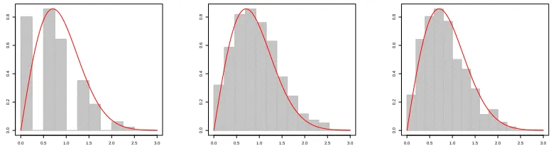
present empirical rates of rejection for the test. We perform 10000 simulations at varying sample sizes of tree—note that Theorem 2 represents a finite sample test. Firstly, Figure 3 plots the histogram of the sum of the edges of the constructed LCA tree; as postulated, the Rayleigh distribution with
scale 1/σoffers a good approximation. Tables 1 and 2 detail the performance of the one-sample most
0.0 0.5 1.0 1.5 2.0 2.5 3.0
0.0
0.2
0.4
0.6
0.8
0.0 0.5 1.0 1.5 2.0 2.5 3.0
0.0
0.2
0.4
0.6
0.8
0.0 0.5 1.0 1.5 2.0 2.5 3.0
0.0
0.2
0.4
0.6
[image:12.612.111.499.239.347.2]0.8
Figure 3. Histograms ofs=e1+· · ·+ek−1from LCA trees of 10000 CGW trees from
π2with number of vertices 10, 100 and 1000 (from left). LCA trees were constructed
by choosing 40% of the vertices randomly from the vertex set of the CGW tree. Solid
red curve is the Rayleigh density with scale 1/√2.
powerful (MP) and Likelihood Ratio (LR) tests. Power calculation is performed only for the LR test since the MP is for simple hypotheses.
H0:π=πσ2 Rejection rate for test of MP test Rejection rate of LR test
10 50 100 10 50 100
π2/3 0.036 0.040 0.047 0.041 0.049 0.050
π1/2 0.071 0.043 0.052 0.067 0.053 0.049
[image:12.612.132.474.479.542.2]π2 0.024 0.047 0.056 0.029 0.049 0.051
Table 1. Level of one sample UMP and LR tests underH0based on the LCA method
for CGW trees with 1000 vertices each from different offspring distributions. LCA trees were constructed by choosing 30% of vertices from the vertex set of each tree at random.
For the two-sample LR test, we generate 1000-vertex CGW trees from different distributions at varying sample sizes and examine the simulation level of the test and its power; these are reported in Tables 3 and 4.
The tests based on the LCA, in general, appear to be performing well with low sample sizes as long as the number of vertices of the CGW trees are large, validating the use of the CRT approach. Since the LCA trees are, in a sense, finite dimensional distributions of the CRT, the tests based on them are able to distinguish between populations of trees quite efficiently.
H0:π1/2 vsH1: Rejection rate for test of LR test
10 50 100
π2/3 0.948 0.964 0.991
π1 0.924 0.967 0.999
[image:13.612.186.423.84.147.2]π2 0.919 0.957 0.987
Table 2. Rejection rate under alternative hypothesis when H0: πσ2 =π1/2 for the
one sample LR test based on the LCA method for CGW trees with 1000 vertices each from different offspring distributions. LCA trees were constructed by choosing 30% of vertices from the vertex set of each tree at random.
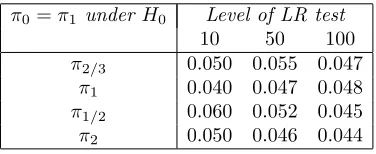
π0=π1 under H0 Level of LR test
10 50 100
π2/3 0.050 0.055 0.047
π1 0.040 0.047 0.048
π1/2 0.060 0.052 0.045
[image:13.612.211.399.224.301.2]π2 0.050 0.046 0.044
Table 3. Level of two-sample LR test underH0based on the LCA method for CGW
trees from two distributions with 1000 vertices each from different offspring distribu-tions. LCA trees were constructed by choosing 30% of vertices from the vertex set of each tree at random.
π0 vsπ1 underH1 Rejection rate for LR test
10 50 100
π2/3 vsπ1 0.508 0.897 0.991
π2/3 vsπ1/2 0.271 0.926 1.000
π2/3 vsπ2 0.781 0.874 0.993
π1 vsπ1/2 0.943 0.982 1.000
π1 vsπ2 0.914 1.000 1.000
π1/2 vsπ2 0.977 0.985 1.000
Table 4. Rejection rate of two-sample LR test under the alternative based on the LCA method for CGW trees from two distributions with 1000 vertices each from different offspring distributions. LCA trees were constructed by choosing 30% of vertices from the vertex set of each tree at random.
5.2. Performance of Dyck path-based tests. In this section we evaluate the performance of the tests based on the random projection method on normalized Dyck paths of CGW trees from Theorems
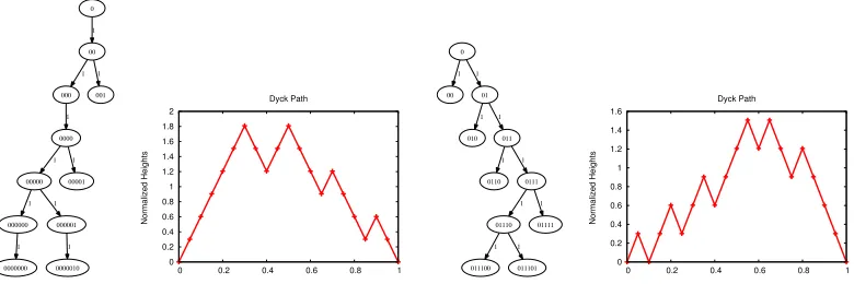
4 and 5. Figure 4 provides an illustration of CGW trees with offspring distributionsπ1/2 andπ1and
their corresponding normalized Dyck paths. Recall that the test statistics were based on the distance from the root of a randomly chosen vertex which is equivalent to the value of the corresponding Dyck path at a randomly chosen point on the x-axis. Figure 5 below plots the histogram of this statistic
scaled byn−1/2 wherenis the number of vertices of the tree for varyingn. This offers verification of
Proposition 5. We now examine the performance of the one-sample and two-sample tests based on the Dyck-path approach and Brownian excursion. Tables 5, 6,7 and 8 tabulate the results.
While the performance of the Dyck path-based tests are acceptable while verifying their attained level of significance, their power under small samples, say 10-20 trees, is quite poor; this can be seen from the power at sample size 10 in Table 8. But upon increasing the sample size to 100 or so, there
[image:13.612.197.411.380.479.2]0 00 1 000 1 001 1 0000 1 00000 1 00001 1 000000 1 000001 1 0000000 1 0000010 1 0 0.2 0.4 0.6 0.8 1 1.2 1.4 1.6 1.8 2
0 0.2 0.4 0.6 0.8 1
Normalized Heights Dyck Path 0 00 1 01 1 010 1 011 1 0110 1 0111 1 01110 1 01111 1 011100 1 011101 1 0 0.2 0.4 0.6 0.8 1 1.2 1.4 1.6
0 0.2 0.4 0.6 0.8 1
Normalized Heights
[image:14.612.111.501.88.218.2]Dyck Path
Figure 4. Left: 11-node CGW tree with offspring distribution π1/2 and its
corre-sponding normalized Dyck path. Right: 11-node CGW tree with offspring distribution
π1 and its normalized Dyck path.
0 1 2 3 4
0.0 0.1 0.2 0.3 0.4 0.5 0.6 0.7
0 1 2 3 4
0.0 0.1 0.2 0.3 0.4 0.5 0.6 0.7
0 1 2 3 4
[image:14.612.113.500.297.406.2]0.0 0.1 0.2 0.3 0.4 0.5 0.6 0.7
Figure 5. Histograms of n−1/2d(root, V) where V is vertex chosen at random on
10000 CGW trees fromπ1/2with number of verticesn= 10, 100 and 1000 (from left).
Solid red curve is the Rayleigh density with scale√2.
H0:π=πσ2 Rejection rate for test of MP test Rejection rate of LR test
10 50 100 10 50 100
π2/3 0.043 0.050 0.049 0.041 0.044 0.052
π1 0.051 0.049 0.046 0.061 0.047 0.049
π1/2 0.046 0.054 0.049 0.057 0.043 0.049
π2 0.047 0.051 0.051 0.049 0.051 0.050
Table 5. Level of one sample UMP and LR tests underH0 based on the Dyck path
method for CGW trees with 1000 vertices each from different offspring distributions.
is marked improvement in the distinguishing power. The fact that the test is based on one randomly chosen vertex, as opposed to LCA subtrees, is reflected in the its minimal utility in small sample sizes.
6. Discussion
Aldous’ papers on the CRT and variants (see, in addition, Aldous [1994a, 1991b]) provide use-ful distributional results and connections to common stochastic processes, which in principle can be harnessed in developing asymptotic statistical tools. The circumscription of our considerations to
H0:π1/2 vsH1: Rejection rate for test of LR test
10 50 100
π2/3 0.262 0.873 0.998
π1 0.197 0.764 0.989
π1 0.441 0.777 0.979
[image:15.612.187.421.84.159.2]π2 0.631 0.816 1.000
Table 6. Rejection rate under alternative hypothesis when H0: πσ2 =π1/2 for the
one sample LR test based on the Dyck path method for CGW trees with 1000 vertices each from different offspring distributions.
π0=π1 under H0 Level of LR test
10 50 100
π2/3 0.056 0.056 0.047
π1 0.052 0.046 0.053
π1/2 0.057 0.051 0.054
[image:15.612.211.399.225.302.2]π2 0.050 0.043 0.052
Table 7. Level of two-sample LR test underH0 based on the Dyck path method for
CGW trees from two distributions with 1000 vertices each from different offspring distributions.
π0 vsπ1 underH1 Rejection rate for LR test
10 50 100
π2/3 vsπ1 0.258 0.833 0.994
π2/3 vsπ1/2 0.169 0.371 0.996
π2/3 vsπ2 0.628 0.999 1.000
π1 vsπ1/2 0.308 0.939 1.000
π1 vsπ2 0.235 0.859 0.994
π1/2 vsπ2 0.817 0.993 1.000
Table 8. Rejection rate of two-sample LR test under the alternative based on the Dyck path method for CGW trees from two distributions with 1000 vertices each from different offspring distributions.
hypothesis testing for distributions is not a shortcoming of the CRT-based approach; rather, as men-tioned in the introduction, this article represents a first step in developing inferential procedures on large tree-structured data. One immediate extension to this work is to approximate distributions of local tree-functionals by corresponding Brownian excursion functional. For example, the Wiener
in-dex of a tree, popular in phylogenetics and chemistry, is exactly 2
nAn where An is the area under
the curve of the Dyck path of a tree with n vertices. The distribution of An can be approximated
by the distribution of Brownian excursion area which is well-know (albeit difficult to compute); see Janson [2012] and references therein for details. Other tree functionals whose limit distributions as Brownian excursion functionals are known include height of a tree, which is the number of generations before extension, maximal distance between a pair of vertices etc. Preliminary investigations based on simulations appear promising.
The ‘weak convergence paradigm’ set forth by Aldous wherein properties (global and local) of ran-dom combinatorial objects likes trees, triangulations, planar maps etc. are studied through continuous approximations offers a fertile ground for development of statistical methodologies on such objects;
[image:15.612.198.411.368.468.2]see Aldous [1994b]. This is an investigative route well worth pursuing in today’s data centric climate wherein complex data structures, modeled in a combinatorial fashion, is prevalent.
On a modeling note, our statistical characterizations of the trees using CRT admits a full likelihood based inference using frequentist and Bayesian techniques. For the latter, a particular context of importance might be regression models that enable modeling of covariate effects on tree-structured
responses. For instance, the offspring varianceσ2 can be modeled as a function of covariates through
parametric and non-parametric prior specifications. This might be particularly appealing in applied contexts where evaluations of systematic variations induced by the covariates are of prime interest. We leave these tasks for future consideration.
7. Appendix
Proof. Proposition 2. First observe that the density in (3.2) implies that the edge lengths are
ex-changeable: s=Pki=1−1ei is invariant to permutations ofei. This implies that the actual labeling to
the vertices and the edges has no relevance to the distribution. For ease of notation, let
Ck=Tk×Rk+−1.
For a tree,τn = (V(τn),E(τn)), with nvertices, we shall consider its LCA tree,LCA(τn, v1, . . . , vk),
constructed fromkvertices, chosen uniformly, withk < n. The question of extendability is basically a
question of whether models specified in terms of joint distributions over a class of index sets isprojective
as defined in eq. 13, p. 92 of Kallenberg [1997]—this is the basis of our definition ofn-extendability.
The probability kernelpk from C1× · · · × Ck−1 to Ck is defined in terms of the conditional density
(ignoring the normalizing factors)
fσ2
LCA(τn, v1, . . . , vk) =·
LCA(τn, v1, . . . , vk−1)
,
which is obtained as
f(LCA(τn, v1, . . . , vk)|LCA(τn, v1, . . . , vk−1)) =
f(LCA(τn, v1, . . . , vk)) f(LCA(τn, v1, . . . , vk−1))
= s
0
se
−(s02−2s2 )σ2,
with s = e1+· · ·+ek−1 and s0 = s+ek. By induction on k, we can extend the existence of the
probability kernelpn toCn with conditional density
f(LCA(τn, v1, . . . , vn)|LCA(τn, v1, . . . , vn−1)) =
s0
se
−(s02−s2 )σ2
2 ,
wheres=e1+· · ·+en−1 ands0 =s+en. By Theorem 5.17 in Kallenberg [1997], we can assert the
existence of the treeτn with distributionp1⊗ · · · ⊗pn; in other words, the distribution on τn can be
defined via the conditional densities as
f(τn) =f(LCA(τn, v1))f(LCA(τn, v2)|LCA(τn, v1))f(LCA(τn, v3)|LCA(τn, v1, v2))
. . . f(LCA(τn, vn)|LCA(τn, v1, . . . , vn−1)).
Straightforward computation with the conditional densities verifies this fact. IfB={v1, . . . , vk}and
V(τn)−B is the set difference, what should be noted is that
X
τ∈V(τn)−B
fσ2(τ) =
Z
ek>0 Z
ek+1>0
. . .
Z
en−1>0
fσ2(τ) dek. . . den−1.
The density on the tree is induced by the density ofswith respect to the Lebesgue measure.
Proof. Proposition 3. SupposeBis a Borel subset ofCn=Tn⊗Rn+−1. Suppose we define a relation∼
on subsetsB1andB2 ofCn asB1∼B2if they containall trees withnvertices; by this we mean that
the “shape” of the tree is disregarded and imply that all trees with n vertices are equivalent. Note
that ∼is an equivalence relation and the generates the quotient classC∼
n = (tn,(e1, . . . , en−1)) with
(e1, . . . , en−1)∈R+n−1 andtn is the canonical tree withnvertices. The Borel sets ofCn∼ are the usual
open rectangles generating the Euclidean spaceRn+−1. Note that the lawPσ2 assigns different mass to
distinct elements inC∼. We are hence interested primarily in Borel subsets ofC∼and will restrict our
examination of distinguishability to this equivalence class.
Suppose the null hypothesis H0 is that σ2 ∈ S0 and the alternative H1 is that σ2 ∈ S1 where
S0∪ S1=S andS0∩ S1=∅. Note that
S=
2,1 2,1,
2 3,
3 4,
4 5, . . .
is a countable set and consequently, so areS0andS1. Furthermore the distribution function associate
withPσ2, for a treeτn, corresponding to the continuous densityfσ2(·)
Fσ2(x1, . . . , xn−1) =
Z x1
0
. . .
Z xn
0
fσ2(τ) de1. . . den
is continuous for each vector (x1, . . . , xn) representing edge lengths. Therefore by part (i) of Theorem
1 in Rao [2000], the proof is complete.
Proof. Theorem 2.
(1) Simple hypotheses:
The key observation here is that conditional onK,s= (s1, . . . , sN) wheresi=e1+· · ·+eki,
is a vector of independent Rayleigh distributed random variables with scale 1/σ. Let us first
perform some calculations in the limit asni→ ∞for eachi= 1, . . . , N. SupposeW1, . . . , WN
are i.i.dR+-valued random variables from a Rayleigh distribution with scale 1/σand density
fσ2(w) =σ
2
we−w
2σ2 2 ,
leading to the likelihood
Lσ2 = (σ2)Nexp
"
−σ 2
2
N
X
i=1
w2
i
#YN
i=1
wi.
Consider
Λ = Lσ21
Lσ2 0
∝exp " PN
i=1w 2
i(σ
2 1−σ
2 0)
2
#
.
By the Neyman-Pearson Lemma (see, p. 60 Lehmann and Romano [2005]), the most powerful test for testingH0 : σ2 =σ20 againstH1 :σ2 =σ21, where σ21 > σ20 is given by the rejection
region
{(w1, . . . , wn) : Λ> Cα}
for a suitable valueCαsuch thatP(Λ> Cα) =αwithP denoting the law corresponding to the
Rayleigh density. Note now that Λ> Cα if and only ifPNi=1w2i < Cα. It is easy to ascertain
thatσ2PN
i=1W 2
i follows a Chi-square distribution with 2N degrees of freedom; therefore the
rejection region defined as
{(w1, . . . , wn) :σ02
N
X
i=1
W2
i < Cα,2N},
whereCα,2N is chosen such thatP(χ2N > Cα,2N) =αwithχ2N denoting a Chi-square random
variable with 2N degrees of freedom, is of sizeα. The power function of the test is
(7.1) θ(N, α, σ2) =Pσ2
N
X
i=1
W2
i < Cα,2N
,
withθ(N, α, σ2
0) =α. For eachi= 1, . . . , N, from discussion earlier, we know thatLCA(τnij, v1, . . . , vki|Ki=
ki) converges in distribution toL(ki), asni→ ∞, with density
fσ2(l(ki)) :=fσ2(e1, . . . , eki−1) =
kYi−1
j=1
1 2j−1
−1
1 2ki−1σ
2s
ie−
σ2s2i
2 .
Note now that a calculation of likelihood ratio forL(ki) using the density above leads to the
exact ratio as Λ. Therefore it is now easy to see that asni→ ∞, for everyi= 1, . . . , N, and
for everyk,
Eπφ(K, N, α, σ2)→θ(N, α, σ2) ∀σ2∈ S,
ensured by the extendability of the class proved in Proposition 2; quite naturally then,
Eπφ(K, N, α, σ20)→θ(N, α, σ20) =α.
(2) Composite hypothesis:
If Wi, i = 1, . . . , N are i.i.d. Rayleigh distributed random variables with scale 1/σ, the it
is easy to determine that the MLE ofσ2 is ˆσ2= 2N
PN
i=1Wi2. The likelihood ratio test, then, is
to rejectH0 if and only if
(σ2 0)Ne−
σ20PN i=1wi2
2
( ˆσ2)Ne−N < β
⇐⇒ te1−tN < β,
wheret = σ20 PN
i=1w 2
i
2 for a suitable β. Observe that the functiong(t) =te
1−t fort > 0;g is
increasing fort <1 and decreasing fort >1. Therefore, the likelihood ratio test is equivalent
to rejectingH0 if and only if
σ20
N
X
i=1
wi2< β1 or σ02
N
X
i=1
w2i > β2;
then, β1 and β2 are determined as in part 1 for the Neyman-Pearson test. Using identical
arguments with power function and weak convergence, as in part 1, the proof is complete.
Proof. Theorem 3. We will work again in the limiting scenario of the Rayleigh densities. In the interests of brevity, we refer the reader to the proof of Theorem 2 for arguments concerning the trees—
they follow along identical lines. SupposeX1, . . . , XN1are i.i.d. from a Rayleigh distribution with scale
1/σ1andY1, . . . , YN1are i.i.d. from a Rayleigh distribution with scale 1/σ2. UnderH0:σ 2
1=σ22=σ2,
the maximum likelihood estimate ofσ2 is
ˆ
σ2=PN2(N1+N2)
1
i=1x 2
i +
PN2
i=1y 2
i .
The maximum likelihood estimates, in general, ofσ2
1 andσ22 are, respectively,
ˆ σ12=
2N1
PN1
i=1x2i
and σˆ22=
2N2
PN2
i=1y2i .
Then likelihood ratio is
Λ = (ˆσ
2)N1+N2
( ˆσ12)N1( ˆσ22)N2
=
N1
N2 + 1
N1+N2
N1
N2
N1 1 +
PN2
i=1y 2
i
PN1
i=1x 2
i
!−N1
1 + PN1
i=1x 2
i
PN2
i=1y 2
i
!−N2
.
Consider now functiong(t) =tN2(1 +t)−(N1+N2) fort >0. Observe thatg(0) = 0 and
g0(t) = t
N2−1
(1 +t)N1+N2
N2−
t(N1+N2)
(1 +t)
,
which is positive (negative) fort >(<)N2
N1, implying thatg(t) is increasing (decreasing) fort >(<)
N2
N1
. Settingt= P
N1
i=1x 2
i
PN2
i=1y 2
i
, it is the case thatt∼N2
N1F2N2,2N1 underH0where σ 2 1 =σ
2
2.
Proof. Proposition 4. First, we need to establish that law on the Brownian excursion is completely
determined by the law of pu(Bex) for a random u on [0,1]. For this we use a result from
Cuesta-Albertos et al. [2006]. It can be checked thatmk=
R
||x||kne(de) fork
∈N, the moments of the scaled
excursion are finite, whereneis the normalized Ito measure of positive excursion of linear Brownian
motion—this is true for everyσ2
∈ S. Now suppose ne1 andne2 are two excursion measures on R+
andneu
1 and neu2 are the randomly projected excursion measures corresponding to the projection pu
whereuis uniform in [0,1]. Consider the set
Eu:={x:neu1(x) =ne
u
2(x)}.
Sinceneis atomless it is the case thatne(Eu)>0 for everyu. Using the so-called Carleman condition
(see, for instance, p. 19 Shohat and Tamarkin [1943]) and Theorem 2.8 from Cuesta-Albertos et al.
[2006], we can claimne1 =ne2. The implication of this is that the distribution of the excursion is
fully determined by just one random projectionpu for a uniformuin [0,1].
Before proving distinguishability, we need to ascertain the density ru
σ2 of pU σ2Bex
= 2
σB ex(U)
whereU is uniform on [0,1]. Note that the density of the Brownian excursion 2
σB
ex at timet
∈(0,1) is given by (see Tak´acs [1991])
(7.2) f(t, x) = x
2σ3
4p2πt3(1−t)3e
−x2σ2
8t(1−t), x >0.
This implies that
ru σ2(x) =
Z ∞
0
f(s, x)ds
=σ2xe−1 2x
2σ2
,
which is a Rayleigh density with scale 1
σ, with continuous distribution function
Ru
σ2(x) = 1−e−
x2σ2
2 .
Bearing in mind that ru
σ2 completely determines the distribution of σ2Bex, from Theorem 1 in Rao
[2000] we have distinguishability. We have omitted details regarding the Borel sets, as detailed in the
proof of Proposition 3, in the interests of brevity.
Proof. Proposition 5. Let Hn be the Dyck path corresponding toτn. Then,d(root, V) is distributed
asHn(2nV). Since for 0≤s≤1,n−1/2Hn(2ns) converges weakly in C[0,1] toBex(s), we can claim
that n−1/2d(root, v) d
→Bex(v) on the set
{V =v}. Using (7.2), we can ascertain the unconditional
density ofBex(V) as
r(x) =
Z ∞
0
f(s, x)ds,