Benchmarking Raspberry Pi 2 Beowulf Cluster

Benchmarking Raspberry Pi 2 Beowulf Cluster

Dimitrios Papakyriakou

mVAS Testing and Deployment

Engineer

COSMOTE Fixed and Mobile

Telecommunications S.A

Athens, Greece

Dimitra Kottou

Core Network Design

Engineer

COSMOTE Fixed and Mobile

Telecommunications S.A

Athens, Greece

Ioannis Kostouros

mVAS Testing and Deployment

Engineer

COSMOTE Fixed and Mobile

Telecommunications S.A

Athens, Greece

ABSTRACT

This paper presents a performance benchmarking of a Raspberry Pi 2 Beowulf cluster. Parallel computing systems with high performance parallel processing capabilities has become a popular standard for addressing not only scientific but also commercial applications. The fact that the raspberry pi is a tiny and affordable single board computer (SBC), given the chance to almost everyone to experiment with knowledge and practices in a wide variety of projects akin to super-computing to run parallel jobs. This research project involves the design and construction of a high performance Beowulf cluster, composed of 12 Raspberry Pi 2 model B computers with CPU 900MHz, 32-bit quad-core ARM Cortex-A7 CPU processors and RAM 1GHz each node. All of them are connected over an Ethernet Network 100 Mbps in a parallel mode of operation so that to build a kind of supercomputer. In addition, with the help of the High Performance Linpack (HPL), we observe and depict the cluster performance benchmarking of our system by using mathematical applications to calculate the scalar multiplication of a matrix, extracting performance metrics such as runtime and GFLOPS.

Keywords

Raspberry Pi cluster, Cluster Computing, Message Passing Interface, High Performance Linpack (HPL), Benchmarking RPi clusters.

1.

INTRODUCTION

We may not have been realized in our mind that our real world is massively parallel, where many complex and interrelated events are happening at the same time. Parallel computing compared to serial computing is much better suited to model, simulate and understand complex real world phenomena, such as Galaxy Formation, Planetary Movements, and Climate Changes. That is to say, when we deal with large and complex problems, it’s impractical or impossible to solve them on a single computer, with given limited RAM memory, and even worst to deal with the so called “Grand Challenge Problems”. In this case we definitely require Petaflops and Petabytes of computer resources to possibly reach a mathematical problem solution.

Nowadays, we all understand that Digital Globalization is the new era of global flows of data information and communication. Internet of Things (IoT) and Clouding are driving data complexity and advanced analytic techniques against large and diverse data sets from different sources. The Big Data era needs to embrace data parallel computing technics so that to increase the efficient data analysis, where data processing and data excavation are the main area in supercomputer applications today. Since supercomputers require an enormous amount of energy to operate, the alternative solution is to use an affordable single board

computer (SBC), such as Raspberry Pi 2 Model B to experiment parallel computing topics.

Raspberry Pi (RPi) 2 Model B “Figure 1” is equipped with a 900 MHz quad-core ARM Cortex-A7 CPU (BCM2836) and 1 GB of RAM (LP DDR2 SDRAM) [1]. The low cost of the Raspberry Pi was the driving force for us to investigate a viable option for building a high performance cluster computer and to study the Pi’s ability to perform in a parallel clustering mode of operation.

An additional motivation for this project is to gain knowledge, experience and understanding of a fully functional clustering computer by the construction and using different benchmarking processes. Moreover, there is an Academic and Professional interest from the authors to investigate later on, how the parallel computing systems can be used for testing purposes in cloud environment.

At this stage in our current project we built a 12 node RPi’s 2 cluster with message passing interface (MPI) configuration so that to measure the performance of the cluster with the High-performance Linpack (HPL) benchmark.

Figure 1: Single Board Computer (SBC) - Raspberry Pi 2 Model B [1].

2.

SYSTEM DESCRIPTION

2.1

Hardware Equipment

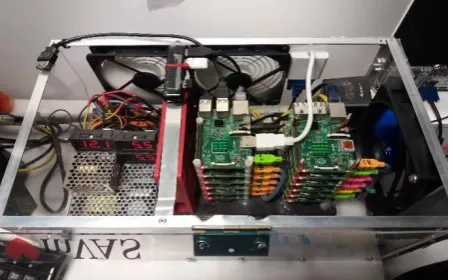
needed to boot it. Moreover, there are 3 USB cords to power the individual Pi’s with 2 switch-mode power supplies of 100W with 5V output boosted to 5.5V so as to adjust the voltage drop. In addition, there are 4 cooling FANs to provide cooling solutions to the system thermal problems and 3 voltage meters to supervise the voltage output of the switch-mode power supplies.

Figure 2: Construction of the Beowulf Cluster.

2.2

Software Tools

The Operating System used to setup the RPi’s in the cluster is the Raspbian GNU/Linux 8 (Jessie) which is one of the official supported Operating System (OS) [2].

The 2nd Software Package we needed to install is the Message Passing Interface (MPI). The MPI is not a library but a standard for development of message-passing libraries based on recommendations of the MPI Forum [3]. There are two prominent implementations of MPI that can be used on the Raspberry Pi. These are: OpenMPI and MPICH. In our case we use MPICH [4], which originally standing for Message Passing Interface Chameleon. It’s an implementation of the MPI standard that supports C, C++ and FORTRAN applications. MPICH is a high performance and wide portable implementation of the Message Passing Interface (MPI) standard.

The 3th software package we needed to install is the (GNU Compiler Collection) GCC Fortran compiler which has optimization and multi-threading features. It’s the default compiler suite in High Performance Computing (HPC). The 4th SW package we needed to install so that to configure properly the cluster is the MPI4PY which stands for MPI for Python. MPI for Python provides MPI bindings for Python. This allows any python program to use a multiple-processor configuration computer. This package is built on top of the MPI-1/2/3 specifications and provides an object-oriented interface for parallel programming in Python. It supports point-to-point (send and receive) and collective (broadcast, scatter and gather) communications for any Python object. Since Message Passing Interface (MPI) is the de facto standard for High Performance Computing (HPC) and parallel programming and the MPI4PY is well-regarded and efficient implementation of MPI for Python, we decided to use this package on the Raspberry Pi for parallel programming. The 6th SW package was the High Performance Linpack (HPL) [5]. The High Performance Linpack benchmark used to measure the performance of a HPC system. It’s used by both the TOP 500 [6] and the Green 500 [7] to compile their rankings. The HPL benchmark is based on the original Linpack benchmark, measuring performance based on solving a system of linear equations using LU factorization [8].

In addition to the above software packages, we lastly needed to load the High Performance Linpack (HPL) software dependency which was the Basic Linear Algebra Subprograms (BLAS). BLAS are a set of well-defined basic linear algebra operations routines to provide standard building blocks so as to perform basic vector and matrix operations [9].

2.3

Design and Setup

The below mentioned “Figure 3” depicts the RPI cluster architecture diagram.

Figure 3: Beowulf cluster architecture diagram

2.3.1

Design

The Cluster design is composed of 12 Raspberry Pi’s connected to the 16-Port 10/100 Mbps Ethernet switch. One out of the 12 Pi is the master or head of the cluster and the rest 11 are slaves or workers. The network configuration is built with static routing namely, each node has a static IP address and the configuration is in such a way where the master can only communicate to every node with secure shell. NFS server shared folder created and configured to both master and slaves Raspberry Pi’s since it’s easier to setup the whole cluster from design point of view. Moreover, there is a sharing internet connection to Raspberry Pi’s meaning that the slave nodes communicate with the Internet via the master node, having the ability to update the operating system with new releases and the RPi’s firmware software as well. As far as the master node is concerned, the boot partition still remains in the microSD card but the root partition is located in the external Hard Disk (HD) with size 320GB. A backup and Shrink procedure to save the master node image is applied prior any significant upgrade and configuration changes so that to be able to reload the previous backup image in case of serious software crash.

2.3.2

Setup

At this stage the cluster can be tested successfully provided that everything is configured correctly. Here, the Network File System (NFS) configuration took place so that to easier configure the High Performance Linpack (HPL).

The last step was to install the High Performance Linpack (HPL) with all the dependencies, such as the Basic Linear Algebra Subprograms (BLAS) development libraries in the master node. In the slave nodes, there is only a need to install the Basic Linear Algebra Subprograms (BLAS) development libraries and nothing more.

3.

PERFORMANCE EVALUATION

The crucial aim of the running tests in the raspberry cluster is to determine if the cluster was scalable, meaning that, if the addition of more cores resulted an addition to the processing capacity of the cluster. Moreover, we had to keep in our mind that each Raspberry Pi comprises a quad-core CPU (4 threads total), meaning that 4 processes can run at the same time per RPi. As a result, 12 Pis comprises 48 cores and as a result 48 processes can be run simultaneously.

3.1

HPL Benchmarks

Broadly speaking, benchmarking is a process of running standard programs to evaluate the speed of a system, where in our case we use the so called High-Performance Linpack (HPL). The Linpack Benchmark is a measure of a computer’s floating rate of execution and determines the upper bound of double precision floating point performance on a distributed parallel system. In other words, measures how fast a computer solves a random dense linear system of equations of order (n), [𝛢 × 𝑥 = 𝑏; 𝐴 ∈ 𝑅𝑛𝑥𝑛_{; 𝑥, 𝑏 ∈ 𝑅}𝑛_{] by first computing the} LU factorization [10], with row partial pivoting of [𝑛 𝑏𝑦 (𝑛 + 1)] coefficient matrix [𝛢 𝑏] = [ L, U y]. Since the lower triangular factor (L) is applied to (b) as the factorization progresses, the solution (x) is obtained by solving the upper triangular system 𝑈 × 𝑥 = 𝑦. The lower triangular matrix (L) is left unpivoted and the array of pivots is not returned. The data is distributed onto a two-dimensional grid of processes (𝑃 𝑏𝑦 𝑄), according to the block-cyclic scheme, to ensure "good" load balance, as well as the scalability of the algorithm [11],[12]. To determine the scalability of the cluster, the problem size or matrix size (N) was kept constant and the number of processors was gradually varied from 4 (1 RPi) to 48 (12 RPi). Since there is no formula mentioned anywhere we run the benchmark several times in order to get the best possible results of HPL benchmark. We had to fine tune several configuration parameters in the HPL.dat file, focusing especially in the Number of problems size (N), the Number of the block size (NBs) in the grid and the Number of process grids (𝑃 × 𝑄) [13].

Briefly, the most important parameters in HPL.dat file that we had to configure are analyzed below:

Number of problems sizes (N). – Parameter (N) specifies the problem size. The aim is to find the largest problem size that fits into the main memory of a specific cluster and for this reason, the main memory capacity for storing double precision (8 Bytes) numbers is calculated. That is to say, in order to get the best performance of the cluster, it’s needed to have the largest problem size that can fix in the entire main RPi memory. We use an “optimal” configuration which is found by the Nelder-Mead tuning method and changes the problem size (N) with other parameters unchanged. The max problem size is calculated as [14] suggests: 𝑁𝑚𝑎𝑥 =

80% 𝑚 × 𝑛where (m) is the free memory in doubles for the machine with the least available free memory and (n) is the number of nodes. The mathematical expression can be seen as such:

Nmax = (Memory in Gbytes × 1024

3 _{× No of Nodes}

8 ) × Z The

(N) in overall must be (80-90) % of the size of the total memory. In particular, in our Raspberry Pi cluster, the maximum possible value for (N) is 32105 (representing approximately the 80% of the available memory) taking into account the 12 RPi nodes, the 4 cores per RPi node, the Memory per Node equal to 1GB and the block size (NB) equal to 128. As a rule of thumb, it’s wise to use the (N) equal to 80% of available memory in order to avoid cluster crash with errors. For a single RPi, Nmax ≈ 11585 × 0.8 = 9268 or alternatively we have the following,: Nmax ≈ 11585 ×

0.9 = 10426.

Number of block size (NBs). – The (NB) is the block size in the grid. HPL uses the block size (NB) for the data distribution and for the computational granularity. Usually block sizes giving good results are within [96, 104, 112, 120, 128… 256] range. The principle is that smaller (NB) gives better load balance from a data distribution point of view, but it’s preferred not to have very large values of (NB). From computational point of view, a too small value of (NB) will probably limit the computational performance. As a result there is a need to apply a trial and error method to find the best approach for better computational performance.

Number of process grids (𝑃 × 𝑄). – (𝑃 × 𝑄) is the size of the grid where P (the number of process rows) and Q (the number of process columns) should be close to being a “square”. According to the developers of the (HPL) in [15], [16] (P) and (Q) should be approximately equal, with Q slightly larger than P which is equal to the number of processors that the cluster has.

Since (N) should be (NB) aligned [17], [18] an additional optimization is needed. For instance, if we consider NB=128, with 12 RPi’s, then (N) is calculated as following:

Nmax = (Memory in Gbytes ×1024

3_{×No of Nodes}

8 ) × Z

Where (Z) is the reduction coefficient, taking values between (80-90) percent, and as a result we have below:

N = (1GB ×10243 ×12

8 ) × 80% = 32105. Considering NB=128, we calculate (32105

128 × 128 = 250.8203125 ≈

250) and next (250 × 128 = 32000). As a result, we optimize the parameters N=32000, NB=128 and 𝑃 × 𝑄 = 48 in the HPL.dat when we run it for the 12 RPi’s. The same optimization logic was applied when executing the benchmark with different values using all the nodes, since there is different proportion of the systems’ total main memory when we use different number of RPi’s in the testing.

3.2

Results

3.2.1

Computing Performance vs. Number of

Node (HPL)

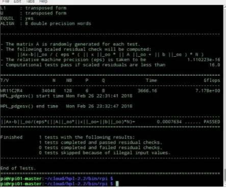
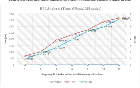
solve the linear system and the achieved GFlops. In “Table 1”, the HPL run with system memory utilization (≈ 80%) compared to what “Table 2” shows up, which is (≈ 85%). The highest performance peaks can be seen in “Figure 4”, and “Figure 5”, respectively in the command line interface as well, whereas “Figure 6” and “Figure 7” depict the cluster performance results in GFlops with 80% and 85% system memory utilization. The theoretical peak performance can be determined by counting the number of floating-point additions and multiplication (in double precision), that can be completed during the cycle time of the machine. The equation (1) which gives the theoretical peak performance is depicted below:

Rpeak GFlops =

Average frequency GHz × No of Cores × operations per cycle (1)

The efficiency of the system in percent is calculated such as 𝑅𝑚𝑎𝑥

𝑅𝑝𝑒𝑎𝑘 × 100 and is dependent on the executed operations. The

ARM Cortex A7 processors, used in our cluster, can process one floating-point addition in one cycle, requiring two cycles for a floating-point multiplication.

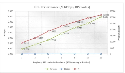
Moreover, the results in “Figure 8” show that increasing the problem size (N), results in a better GFlops performance. At the same time we notice that increasing the problem size (N) and the RPi’s in the testing, results an increasing of the speedup of the system which can be seen easily in the “table 1” and “table 2” as well. Apart from the cluster performance in GFlops, the investigation of the speedup when we add gradually RPi nodes in the test was a research question to be answered. The speedup (Sp) that can be achieved when the

testing is run and can be defined with equation (2) as following:

𝑆𝑝 = 𝐹𝑝 𝐹1 (2)

Where (F1) is the GFlops on a single-processor system and

(Fp) is the GFlops on a multiprocessor system. The theoretical

maximum speedup is equal to the number of single-processor nodes. That is to say, for the two RPi nodes the value is 2, for the four nodes the value is 4 and so on. The “Table 1” and “Table 2” depicts the experimental results of the HPL benchmarking testing. It can be seen the increased speedup performance achieved by (HPL) testing when we gradually increase the RPi Nodes from 1 to 12 in the cluster. The outcome of the (HPL) is exactly what we were expecting since the increased RPi’s means increased processors in the testing.

Table 1. Beowulf cluster setup parameters and testing results with 80% system memory utilization

System Memory

utilized

N Nodes used

NB Time

[sec] GFlops Speedup

≈ 80%

9216 1 128 587.51 0.888 1.00

13056 2 128 842.38 1.762 ≈1.98 18560 4 128 1640.98 2.598 ≈ 2.92 22656 6 128 2028.69 3.822 ≈ 4.30 26240 8 128 2446.26 4.924 ≈ 5.54 29312 10 128 2938.29 5.715 ≈ 6.43 32000 12 128 3137.71 6.963 ≈ 7.84

Table 2. Beowulf cluster setup parameters and testing results with 85% system memory utilization.

System Memory

utilized

N Nodes used

NB Time

[sec] GFlops Speedup

≈ 85%

9984 1 128 702.79 0.944 1.00 13952 2 128 1021.63 1.773 ≈ 1.87 19712 4 128 1905.89 2.679 ≈ 2.83 24192 6 128 2373.69 3.977 ≈ 4.21 27904 8 128 2742.70 5.282 ≈ 5.59 31104 10 128 3385.03 5.927 ≈ 6.27 34048 12 128 3666.16 7.178 ≈ 7.60

Figure 4: Highest measured cluster performance results in GFlops with 80% system memory utilization.

Figure 4: HPL cluster performance results in GFlops with 80% system memory utilization (4 threads per node)

Figure 5: HPL cluster performance results in GFlops with 85% system memory utilization (4 threads per node) 587.51

842.38

1640.98

2028.69

2446.26

2938.29

3137.71

0.888

1.762

2.598

3.822

4.924

5.715

6.963

0.000 1.000 2.000 3.000 4.000 5.000 6.000 7.000 8.000

0 500 1000 1500 2000 2500 3000 3500

1 2 4 6 8 10 12

G

Flo

p

s

Time

(se

c)

Raspberry Pi 2 Nodes in Cluster (80 % memory utilization)

HPL Analysis (Time, GFlops, RPi nodes)

Nodes Time GFlops

702.79

1021.63

1905.89

2373.69

2742.7

3385.03

3666.16

0.944

1.773

2.679

3.977

5.282

5.927

7.178

0 1 2 3 4 5 6 7 8

0 500 1000 1500 2000 2500 3000 3500 4000

1 2 4 6 8 10 12

G

Flo

p

s

Time

(se

c)

Raspberry Pi 2 Nodes in Cluster (85% memory utilization)

HPL Analysis (Time, GFlops, RPi nodes)

Figure 6: HPL cluster performance results compared to increased problem size (4 threads per node)

4.

CONCLUSION

In this project, we implemented and analyzed the performance of a cluster with low cost, with embedded ARM processors and Raspberry Pi 2 platform by using the HPL benchmark. After performing this work, we can state the following observations: (a) the increase of the number of processors or the number of the RPi nodes, resulted a considerable increase in the peak performance in GFlops; (b) the increase of the RPi nodes resulted a considerable increase in speedup of the cluster; (c) In addition, increasing the problem size (N) resulted in a better GFlops performance; (d) after the analysis and the results obtained by running the HPL benchmark, we can conclude that the ARM processors performed well when running parallel applications. Apparently, such an RPi cluster cannot be used for scientific research as a large scale supercomputer, but can be used for Academic educational reasons with no doubts. (e) We have noticed that with increasing the system memory utilization from 80 % into 85%, the performance in GFlops had been better –or slightly better- as expected to be, but the speedup was not. The explanation could be that the on-board (10/100 Mbps) Ethernet limits the cluster ability to outperform due to interconnection limits, meaning how quickly nodes/processes could communicate with each other. Obviously, the limitation of the 1 GB memory is an obstacle to achieve better performance but the cluster is scalable with no doubts. Despite the limitations the RPi’s depicted, since it’s a single board computer (SBC) with embedded RAM, the Beowulf cluster can be used in a professional manner for automation testing purposes. In our job, we are moving from manual testing to automation testing procedures with agile methodologies. The parallel computing systems can be used as a centralized architecture to perform, in a large scale, automation testing in cloud environment with Internet of Things (IoT) applications by using for instance Python programming. This idea has been applied successfully by the

authors in functional testing used in the Telecom sector and in particular in Value Added Services (VAS) Nodes. Linux and Python used with incredible performance in limited functional tests, using the parallel computing feature itself to increase the performance or in a way where the master node guides the clients to perform different set of testing batches, in different Telecom nodes at the same time.

In addition, for the authors the project had been extremely educational to see in practice how to build and analyze a parallel computing system with low cost and affordable single board computers (SBCs) and how the parallel computing systems can be used for testing purposes.

5.

FUTURE WORK

Since our primary job is the design, testing and deployment in the Telecom Core Network and Value Added Services (VAS) domain, we are very interested in researching the Telecom cloud environment with High Performance Parallel Computing Systems. Our first attempt was to design and deploy an affordable parallel computing system using Raspberry’s Pi 2 so that to move forward a few steps the idea of using cluster architectures in automation testing. The next step is to carry on with building a High Performance Hadoop cluster so that to research and analyze the cluster processing capabilities of large amount of data under the scope of Big Data Analytics. The Internet of Things (IoT) is served by cloud environments producing huge amount of data, especially in the Telecom sector where High Performance Computing Systems are needed and in turn there is a challenge opportunity to investigate not only the design and architecture but also the Automation Testing Methodologies in clouding.

6.

ACKNOWLEDGMENTS

We express our sincere gratitude to all multi Value Added Services (mVAS) team for the precious suggestions, 0.888

1.762

2.598

3.822

4.924

5.715

6.963

9216

13056

18560

22656

26240

29312

32000

0 5000 10000 15000 20000 25000 30000 35000

0.000 1.000 2.000 3.000 4.000 5.000 6.000 7.000 8.000

1 2 4 6 8 10 12

Prob

le

m

Siz

e

(N)

G

Flo

p

s

Raspberry Pi 2 nodes in the cluster (80% memory utilization)

HPL Performance (N, GFlops, RPi nodes)

27 motivation and knowledge contribution for the successful

completion of this project.

7.

REFERENCES

[1] Raspberry Pi 2 Model B. [Online]. Available: https://www.raspberrypi.org/products/raspberry-pi-2-model-b/

[2] Raspberry Pi 2 Model B. Operating System. [Online]. Available: https://www.raspberrypi.org/downloads/ [3] MPI. MPI Forum. [Online]. Available:

http://mpi-forum.org/

[4] MPI. MPICH. [Online]. Available: https://www.mpich.org/

[5] Netlib. HPL. [Online]. Available: http://www.netlib.org/benchmark/hpl/

[6] Top500.org. Top500 lists. [Online]. Available: https://www.top500.org/.

[7] Green500.org. Green500 lists. [Online]. Available: https://www.top500.org/green500/.

[8] LU factorization. [Online]. Available: https://www.geeksforgeeks.org/l-u-decomposition-system-linear-equations/

[9] Netlib. Netlib blas, [Online]. Available: http://www.netlib.org/blas/.

[10]Mathematics. LU Decomposition of a System of Linear

Equations. [Online]. Available:

https://www.geeksforgeeks.org/l-u-decomposition-system-linear-equations/

[11]Dunlop, D., Varrette, S. and Bouvry, P. 2010. Deskilling HPL, Vol. 6068 of Lecture Notes in Computer Science, Springer, Heidelberg, Berlin, 102–114.

[12]Luszczek, P., Dongarra, J., Koester, D., Rabenseifner, R., Lucas, B., Kepner, J., McCalpin, J., Bailey, D. and Takahashi, D. 2005. Introduction to the HPC Challenge Benchmark Suite, Technical Report, ICL, University of Tennessee at Knoxville.

[13]Netlib. HPL Tuning.

http://www.netlib.org/benchmark/hpl/tuning.html#tips [14]Dunlop, D., Varrette, S. and Bouvry, P. 2008. On the use

of a genetic algorithm in high performance computer benchmark tuning, Proceedings of the International Symposium on Performance Evaluation of Computer and Telecommunication Systems, SPECTS 2008, Art. No.:4667550, 105-113.

[15]HPL Frequently Asked Questions. [Online]. Available: http://www.netlib.org/benchmark/hpl/faqs.html

[16]Sindi, M. 2009. HowTo – High Performance Linpack (HPL), Technical Report, Center for Research Computing, University of Notre Dame.

[17]Petitet, A., Whaley, R. C., Dongarra, J., and Cleary, A. HPL - a portable implementation of the high- performance linpack benchmark for distributed-memory computers. http://www.netlib.org/benchmark/hpl/ [18]Cox J. Simon, Cox T. James, Boardman P. Richard,

Johnston J. Steven, Scott Mark, and Neil S. O’Brien. Iridis-pi: a low-cost, compact demonstration cluster. Cluster Computing 17, no. 2 (June 22, 2013): 349-58. doi: 10.1007/s10586-013-0282-7.