Temporal difference Learning with Sampling Baseline for Image Captioning

Temporal-difference Learning with Sampling Baseline for Image Captioning

Hui Chen

, Guiguang Ding

, Sicheng Zhao

, Jungong Han

†_{School of Software, Tsinghua University, Beijing 100084, China}

‡_{School of Computing and Communications, Lancaster University, Lancaster, LA1 4YW, UK}

{jichenhui2012,schzhao,jungonghan77}@gmail.com, [email protected]

Abstract

The existing methods for image captioning usually train the language model under the cross entropy loss, which results in the exposure bias and inconsistency of evaluation metric. Recent research has shown these two issues can be well ad-dressed by policy gradient method in reinforcement learning domain attributable to its unique capability of directly opti-mizing the discrete and non-differentiable evaluation metric. In this paper, we utilize reinforcement learning method to train the image captioning model. Specifically, we train our image captioning model to maximize the overall reward of the sentences by adopting the temporal-difference (TD) learn-ing method, which takes the correlation between temporally successive actions into account. In this way, we assign dif-ferent values to difdif-ferent words in one sampled sentence by a discounted coefficient when back-propagating the gradien-t wigradien-th gradien-the REINFORCE algorigradien-thm, enabling gradien-the correlagradien-tion between actions to be learned. Besides, instead of estimating a “baseline” to normalize the rewards with another network, we utilize the reward of another Monte-Carlo sample as the “baseline” to avoid high variance. We show that our proposed method can improve the quality of generated captions and outperforms the state-of-the-art methods on the benchmark dataset MS COCO in terms of seven evaluation metrics.

Introduction

Scene understanding is one of the ultimate goals of computer vision. Image captioning aims at generating reasonable cap-tions automatically for images which is of great importance to scene understanding. It is a challenging task not only be-cause the captioning models must be capable of recognizing what objects are in the image, but also must be powerful e-nough to understand the semantic relationships among the objects and describe them properly in natural language. It is also of great significance to enable machine mimicking the human ability to express the rich visual information with descriptive language, and thus attracts much attention from academic researchers and industry companies.

∗

This research was supported by the National Natural Science Foundation of China (Grant Nos. 61571269, 61701273), the Royal Society Newton Mobility Grant (IE150997) and the Project Funded by China Postdoctoral Science Foundation (No. 2017M610897). Corresponding authors: Guiguang Ding and Jungong Han. Copyright c2018, Association for the Advancement of Artificial Intelligence (www.aaai.org). All rights reserved.

Inspired by the machine translation domain, recent works focus on the deep network based and end-to-end method-s mainly under the encoder-decoder framework. In general, the recurrent neural networks (RNN), especially long short term memory (LSTM) (Hochreiter and Schmidhuber 1997), are employed as the decoder to generate captions (Vinyals et al. 2015; Jin et al. 2015; Xu et al. 2015; You et al. 2016; Zhao et al. 2017) on the basis of the visual features of im-age extracted by the CNN. These models are usually trained to maximize the likelihood of next ground-truth word giv-en the previous ground-truth words. However, this method will lead to a problem calledexposure bias(Ranzato et al. 2015), since at test time, the model uses the word sampled from the model predictions as the next LSTM input, instead of the ground-truth words. The second problem is about the inconsistency between the optimizing function at training time and the evaluation metrics at test time. The training procedure attempts to lower the cross entropy loss, while the metrics used to evaluate a generated sentence are some discrete and non-differentiable NLP metrics such as BLEU, ROUGE, CIDEr, and METEOR. These two problems limit the ability of the model to understand the image and describe it with descriptive sentences.

of RNN like Ranzato et al. did. This method usually exhibits high variance, thus making the training unstable.

In this paper, we apply the temporal difference method (Sutton 1988) to model the RL value function, instead of the monte carlo rollouts, because the monte carlo rollouts method only learns from the observed values, meaning that the value can not be obtained until the sequence is finished. Differently, the temporal difference method assumes that there are correlations between temporally successive action-s, thuaction-s, it can estimate the value of actions based on the pre-viously learned estimates of the successive actions by means of the dynamic programming idea. Since the context of the sentence has a strong correlation, we assume that the tempo-ral difference learning could be more appropriate to model the value function. Besides, to reduce the variance during the model training, we also use the baseline suggested by (Ren-nie et al. 2017) where they consider the caption generated by the test-time inference algorithm to be the baseline caption. However, we notice that the way of baseline in (Rennie et al. 2017) can not approximate the value function correctly, because the test-time inference algorithm tends to pick the fairly good sentence which is better than the sentence sam-pled from the model distribution in most cases. Instead, we generate two sentences both sampled from the model distri-bution with the idea that the quality of actions sampled from the same distribution in multinomial sample policy are close in terms of the probability. Therefore, we adopt one of the two sentences as the baseline sequence, and apply the tem-poral difference method.

Overall, the contributions of this paper are three-fold: • We directly optimize the evaluation metrics during

train-ing through a temporal difference method in reinforce-ment learning where each action at different time step has different impacts on the model.

• To avoid the high variance during the training, we employ a novel baseline modelling method by using a sequence sampled from the same distribution as the sequence for gradient to calculate the baseline.

• We conduct a massive of experiments and comparisons with other methods. The results demonstrate that the pro-posed method has a significant superiority over the-state-of-the-art methods

Related Work

The literature on image captioning can be divided into three categories based on different ways of sequence gen-eration (Jia et al. 2015): template-based methods (Farhadi et al. 2010; Kulkarni et al. 2011; Elliott and Keller 2013), transfer-based methods (Gong et al. 2014; Devlin et al. 2015; Mao et al. 2015) and the neural network-based methods. S-ince the proposed method adopts the same framework as the neural network-based methods, we mainly introduce the re-lated works about image captioning with them.

The neural network-based methods get inspirations from machine translation (Schwenk 2012; Cho et al. 2014) where two RNNs are used as the encoder and the decoder respec-tively. Vinyals et al. (2015) replaced the RNN encoder with a deep CNN, and adopted the LSTM to decode the image

vector to a sentence. This work achieved a reasonable re-sult and hereafter there are many works following this idea and studying further. Xu et al. (2015) applied the attention mechanism in the image captioning task in which the de-coder can function as the human’s eye focusing its atten-tion on different regions of the image at each time step. Lu et al. (2017) improved the attention model by introducing a visual sentinel allowing the attention module adaptively attend to the visual regions. You et al. (2016) proposed a se-mantic attention model which selectively attends to sese-mantic concept regions by fusing the global image feature and the semantic attributes feature from an attribute detector. Chen et al. (2017a) proposed a spatial and channel-wise attention model to attend to both image features and visual regions adaptively.

Recently, researchers made efforts to incorporate re-inforcement learning into the standard encoder-decoder framework to address the exposure bias and the non-differentiable metric issues. Specifically, (Ranzato et al. 2015) used the REINFORCE algorithm (Williams 1992) and proposed a novel training method at sequence level direct-ly optimizing the non-differentiable test metric. (Liu et al. 2016) applied the policy gradient algorithm in the training procedure for image captioning models, in which the word-s word-sampled from the current model at each time word-step were awarded with different future rewards via averaging the re-wards of some Monte-Carlo samples. A simple MLP was used to produce the estimate of the future reward, and such estimate will in turn be treated as the baseline to reduce the variance. Self-critical sequence training (SCST) (Rennie et al. 2017) adopted the policy gradient algorithm as well but the difference from (Liu et al. 2016) is that SCST just ran the LSTM forward process twice and obtained two sequences, one generated by running the inference algorithm at test time and the other sampled from the multinomial strategy. SCST made the reward of the sequence from the inference algo-rithm as a baseline to reduce the training variance.

CNN …

Training Set

LS

TM

LS

TM

𝑤1𝑠 sample

LS

TM

𝑤𝑇𝑠

R

ew

ar

d

𝑟𝑠_{− 𝑟}𝑠′

𝜸𝑇−𝑡−1_𝑟𝑠_{− 𝑟}𝑠′

𝜸𝑇−1_𝑟𝑠_{− 𝑟}𝑠′ BP

sample

BP

𝑤𝑡𝑠

LS

TM

LS

TM

𝑤1𝑠′ sample

LS

TM

𝑤𝑇𝑠′

𝑤𝑡𝑠′

sample

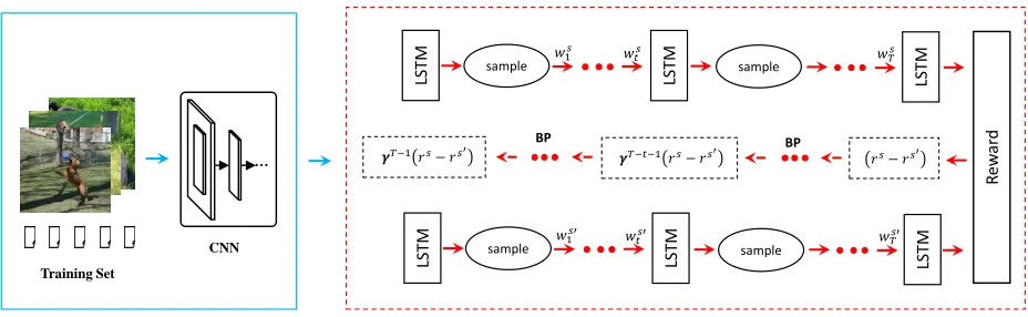
Figure 1: The framework of the proposed model, including two parts: the encoder (in blue rectangle) and the decoder (in red rectangle). The top and bottom LSTMs share the same parameters. The right arrow means the forward operation and the left arrow means the backward operation.Ws_{= (w}s

1, ws2, ..., wsT)andW

s0 _{= (w}s0 1, ws

0 2, ..., ws

0

T)are two sampled sequences from

the model in multinomial policy.rs_andrs0_{are the rewards of sequencesW}s_andWs0_{, respectively.γis a discounted coefficient}

in temporal difference method.stis the output of the softmax function.

Methodology

Encoder-Decoder framework

Given an imageI, the image captioning model needs to gen-erate a caption sequenceW = {w1, w2, ..., wT}, wt ∈ D

whereD is the vocabulary dictionary. We adopt the stan-dard CNN-RNN architecture for image captioning. CNN, which can be seen as an encoder, encodes an input image into a vector. RNN functions as a decoder aiming to gen-erate the captions given the image feature. Here, we use L-STM (Hochreiter and Schmidhuber 1997) as the decoder. During generation, LSTM generates a word at each time step conditioned on the previously generated words wt−1,

the previous hidden stateht−1 and the context vectorct−1

containing the context information that LSTM has seen. The LSTM updates the hidden units and cells as follows:

x−1=CN N(I), x0=E(w0) xt=E(wt)

it=σ(Wixxt+Wihht−1+bi)(input gate) ft=σ(Wf xxt+Wf hht−1+bf)(forget gate) ot=σ(Woxxt+Wohht−1+bo)(output gate)

ct=itφ(Wzx⊗xt+Wzh⊗ht−1+bc⊗) +ftct−1 ht=ottanh(ct)

qt=Wqhht

(1)

wherew0 is a special token indicating the start of the

se-quence,CN N(I)is the feature extractor for imageI,E()

is the embedding function which maps the one-hot repre-sentation of a word into the embedding semantic space. We initialize thec0andh0to the zero vector.

Then a distribution over the next word wt will be

pro-duced by using the softmax function:

wt∼Sof tmax(qt) (2)

The likelihood of a wordwtat time steptis decided by a

conditional probability conditioned on the input imageIand

previous words w0, w1, ...wt−1: p(wt|I, w0, w1, .., wt−1). So the probability of a generated sequence W = (w0, w1, w2, .., wT) given the input image I will be the

product of the conditional probability of each word:

p(W|I) = T Y

t=0

p(wt|I, w0, w1, ..., wt−1) (3)

Show and tell paper (Vinyals et al. 2015) uses the cross-entropy loss (XENT) to train the whole network. The XENT loss maximizes the probability of the descriptionW gener-ated by the model, which intends to minimize:

L=−

T X

t=0

logp(wt|I, w0, w1, ..., wt−1) (4)

The XENT loss will lead the model to generate the word with the highest posteriori probability at each time step t

without considering the quality of the whole sequence at test time and cause a phenomena called search error (Ranzato et al. 2015).

Temporal difference learning: TD(λ)

Reinforcement learning can provide solutions for decision-making problem. We consider the image captioning task as a decision-making problem or a finite Markov process (MDP). In the MDP setting, the state can be defined as the informa-tion that has known at the current time step. So we consider the statestas a list consisting of the image and the previous

words:

st={I, w0, w1, ..., wt−1} (5)

And the action is the input image or the word generated at different time step. The parameter of the network,θ, defines the policy networkpθ which will produce an action

an “action” (image feature and words) in guidance of the ac-tion distribuac-tion. After each acac-tionat, the LSTM updates its

internal parameters to increase or decrease the probability of taking the action at according to the reward. “Reward”

is an important element in RL, which decides the evolution direction of the agent. Here, we define the reward as the s-core computed by evaluating the generated captions using the corresponding ground-truth sequences under the stan-dard evaluation metrics, such as BLEU-1,2,3,4,CIDEr, ME-TEOR, etc. We denote the reward byrin the following.

In reinforcement learning, the agent’s task is to maximize the total amount of rewards passing from the environment to the agent. For image captioning, the reward will not be calculated until the EOS, a special token indicating the end of the sequence, is generated by the model. Therefore, it is necessary to define the reward function for each word. In this paper, we define the reward for each wordwtas follows:

rt=

r t=T

0 t <T (6)

whereris the score calculated using the evaluation metrics andT is the final time step.

The agent aims to maximize the cumulative rewards it re-ceived in the long run. For an episode(a0, a1, ..., aT), we

define the Q-value functionQ(st, at+1)as a function of the

current statestof the model and some possible actionat+1

to estimate the expected future reward. There are many ways to define the Q-value function. (Liu et al. 2016) exploited Monte Carlo rollouts method in which the model will gener-ate many sequences and used the average of rewards of these sequences as the Q-value. While in this paper, we adopt the temporal-difference (TD) learning to estimate Q-value func-tion.

In temporal difference learning, n-step expected return

Gt:t+n is defined as the sum of the next n rewards plus the

estimated value of the next(n+ 1)’th state, each appropri-ately discounted, in n-step TD method:

Gt:t+n=rt+1+γrt+2+...+γn−1rt+n+γnV(st+n) (7)

where0 ≤t ≤T −n. The n-step expected return can be viewed as a n-step backup starting from current time step

t. And the Q-value is a weighted average of a few n-step back-ups in the TD(λ) method, in which all weights sum to 1. Specifically, the Q-value in TD(λ) is defined as follows:

Q(st, at+1) = (1−λ)

∞

X

n=1

λn−1Gt:t+n (8)

Since the length of generated sequence has limitT in im-age captioning, we have:

Q(st, at+1) = (1−λ) T−t−1

X

n=1

λn−1Gt:t+n+λT−t−1Gt (9)

whereλis the trad-off parameter which decides how much the model depends on the current expected returnGt. Here,

we setλ = 1for our image captioning model. Then, with

λ= 1, Eq. (6) and Eq. (7), we have:

Q(st, at+1) =γT−t−1r (10)

Now, we define the RL loss function as follows:

L(θ) =−EWs_∼p θ[

T X

t=0

Q(st, at+1)] (11)

whereWs _{= (w}s

0, ws1, ..., wsT)andwtsis sampled from the

model at time stept. The gradient∇L(θ)can be calculated as in REINFORCE algorithm (Williams 1992):

∇L(θ) =−EWs_∼pθ[ T X

t=0

Q(st, at+1)∇θlogpθ(Ws)]

(12) In practice, Eq. (12) can be approximated using one se-quence generated by the network using the Monte-Carlo sample method for each training sample. So we have:

∇L(θ) =−

T X

t=0

Q(st, at+1)∇θlogpθ(Ws)

=−

T X

t=0

γT−t−1r∇θlogpθ(Ws)

(13)

The definition of Q-value above makes the estimator with high variance. In order to reduce the variance during train-ing, we introduce the baseline. (Rennie et al. 2017) used the reward of the sequence obtained by the current model with the greedy sampling strategy. (Liu et al. 2016) used an MLP to estimate the baseline reward. In this paper, we intro-duce a new baseline strategy similar to (Rennie et al. 2017) where the difference is that we use a sequence obtained with a multinomial sampling strategy. Then the gradient function will be as follows:

∇L(θ) =−

T X

t=0

γT−t−1(r−rbaseline)∇θlogpθ(Ws)

(14) In fact, the two sequences, one for gradient and the oth-er for baseline, are both genoth-erated by the current network

pθ with a multinomial sampling strategy. The idea is that

the difference between rewardrandrbaselineis small since

they are computed by two sequences which are both sam-pled from the same distribution and this will achieve a lower variance during training than the way in (Rennie et al. 2017) resulting in a more stable parameters updating.

Then according to the chain rule, the final gradient will be as follows:

∇L(θ) =−

T X

t=0 ∂L(θ)

∂qt ∂qt

∂θ (15)

whereqtis the input of the softmax function at time stept

and

∂L(θ) ∂qt

=γT−t−1(r−rbaseline)(1ws

t −pθ(wt|ht)) (16)

hidden vectors for language model. Next, at each time step, the LSTM will be fed in the word sampled from the curren-t model acurren-t lascurren-t curren-time scurren-tep, excepcurren-t acurren-t curren-the 0curren-th curren-time scurren-tep, uncurren-til a special token EOS is generated. The model will generate two sequences,WsandWs0, sampled in multinomial pol-icy. The gradient put on words ofWs_{is determined by the}

difference between the rewards ofWs_andWs0_{. This can}

lower the variance of the gradients and makes the training procedure stable.

Experiments

Dataset and setting

We evaluate our proposed method on the popular MS CO-CO dataset (Lin et al. 2014). MS CO-COCO-CO dataset contain-s 123,287 imagecontain-s labeled with at leacontain-st 5 captioncontain-s includ-ing 82783 traininclud-ing images and 40504 validation images. MS COCO provides 40775 images as test set for online evalu-ation as well. Since the standard test set is not public, we use 5000 images for validation, 5000 images for test and the remains for training, as in previous works (Xu et al. 2015; You et al. 2016; Chen et al. 2017c) for offline evaluation. We use the code publicly1to preprocess the dataset, such as pruning infrequent words, and we end up with a vocabulary set which has 9567 different words. We use different metric-s, including BLEU-1, BLEU-2, BLEU-3, BLEU-4, METE-OR, ROUGE-L and CIDEr, to evaluate the proposed method and compare with other methods.

We extract the image’s feature in two different ways. In the first way, the image is encoded as a global feature vector of dimension 2048, and during training, the image feature vector is only fed into the LSTM unit at the beginning. In the second, the full image is encoded with the final convolu-tional layer of Resnet-101 and ends up with a7×7×2048

feature map, and at each time step, this feature map will be input into the LSTM units. In the following, we denote the models with image features obtained in the first way as the FCmodels, and those in the second way asattention(att) models.

Implementation Details

We use ResNet-101 (He et al. 2016) pretrained on ImageNet to encode images. All images are preprocessed as follows: scaling the smaller edge to 256, doing color normalization and cropping to centered rectangle. The decoder is a one-layer LSTM with a hidden state size of 512. The embedding dimension of word is fixed to 512. We set the embedding di-mension of image feature to 512 using a linear layer. When training the attention model, the parameter updating of L-STM follows (Rennie et al. 2017). We train models under the XENT loss using ADAM optimizer with a learning rate of5×10−4_{and finetune the CNN from the beginning. We}

then train the models under the reinforcement loss to opti-mize the CIDEr-D metric without finetuning. For all models, the batch size is set to 16 and every 1K iterations the model evaluation will be performed during training. When train-ing models under the RL loss, the learntrain-ing rate for language

1

https://github.com/karpathy/neuraltalk

model is initialized to1×10−4and set to5×10−5after 50K iterations, then decreased1×10−5_{every 100K iterations}

un-til1×10−5_{. When training models using RL loss, we use}

the models trained under XENT loss as pretrained models to reduce the search space. By default, the beam search size is fixed to 3 for all models for test.

Performance on MS COCO

Performance of our models. To test the effectiveness of TD(λ) modelling method and the baseline method we pro-posed, we conduct a series of experiments for image cap-tioning on karpathy’s split of MS COCO dataset. The con-figurations of models are listed as follows:

• XENT-FC: the FC model trained with the XENT loss. • SR-Greedy-FC: the FC model trained with a shared

re-ward for every word in a sampled sentence.

• TD-Greedy-FC: the FC model trained with TD learning and the baseline is computed by the reward of the se-quence sampled from the greedy policy.

• TD-Multinomial-FC: the attention model trained with TD learning and the baseline is computed by the reward of the sequence sampled from the multinomial policy.

The results of these four models above are listed in Ta-ble 1. The model in the first row is trained with the XENT loss and three models in the second row are trained with the reinforcement learning. Through comparing the result of the XENT-FC with the three RL models in the second row, we can find that our proposed method with the reinforcemen-t learning can improve reinforcemen-the performance areinforcemen-t a greareinforcemen-t margin. Compared with the performance of the SR-Greedy-FC mod-el, the TD-Greedy-FC model performs better in all metrics, indicating the effectiveness of the TD(λ) modelling method. The TD-Multinomial-FC model achieves an improvemen-t of 1.1% and 2.4% in improvemen-terms of improvemen-the CIDEr meimprovemen-tric com-pared with the TD-Greedy-FC model and SR-Greedy-FC model respectively. Better performance can be attributed to the TD(λ) modelling method which approximates different actions with the discounted expected future reward and the baseline method we proposed which can make the variance more lower than the method that uses the sampled sequence from a greedy policy as the baseline sequence.

Table 1: Performance of the proposed method on MS COCO dataset.

BLEU-1 BLEU-2 BLEU-3 BLEU-4 METEOR ROUGE-L CIDEr

XENT-FC 72.6 55.5 41.5 31.1 25.2 53.3 96.3

SR-Greedy-FC 75.1 58.6 43.8 32.5 25.5 54.4 107.4

TD-Greedy-FC 75.6 59.2 44.5 33.1 25.7 54.9 108.7

TD-Multinomial-FC 75.9 59.5 44.6 33.1 26.0 54.9 109.8

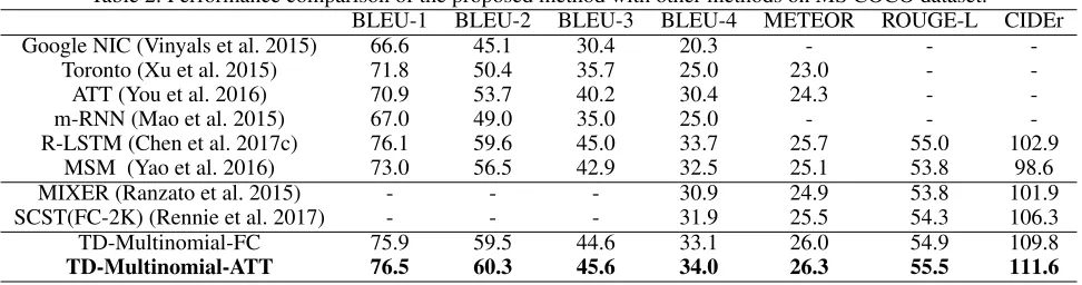
Table 2: Performance comparison of the proposed method with other methods on MS COCO dataset.

BLEU-1 BLEU-2 BLEU-3 BLEU-4 METEOR ROUGE-L CIDEr

Google NIC (Vinyals et al. 2015) 66.6 45.1 30.4 20.3 - -

-Toronto (Xu et al. 2015) 71.8 50.4 35.7 25.0 23.0 -

-ATT (You et al. 2016) 70.9 53.7 40.2 30.4 24.3 -

-m-RNN (Mao et al. 2015) 67.0 49.0 35.0 25.0 - -

-R-LSTM (Chen et al. 2017c) 76.1 59.6 45.0 33.7 25.7 55.0 102.9

MSM (Yao et al. 2016) 73.0 56.5 42.9 32.5 25.1 53.8 98.6

MIXER (Ranzato et al. 2015) - - - 30.9 24.9 53.8 101.9

SCST(FC-2K) (Rennie et al. 2017) - - - 31.9 25.5 54.3 106.3

TD-Multinomial-FC 75.9 59.5 44.6 33.1 26.0 54.9 109.8

TD-Multinomial-ATT 76.5 60.3 45.6 34.0 26.3 55.5 111.6

Table 3: Evaluation on the online MS COCO testing server.†indicates the results of ensemble models. BLEU-1 BLEU-2 BLEU-3 BLEU-4 METEOR ROUGE-L CIDEr c5 c40 c5 c40 c5 c40 c5 c40 c5 c40 c5 c40 c5 c40 MSM†(Yao et al. 2016) 73.9 91.9 57.5 84.2 43.6 74.0 33.0 63.2 25.6 35.0 54.2 70.0 98.4 100.3 R-LSTM (Chen et al. 2017c) 75.1 91.3 58.3 83.3 43.6 72.7 32.3 61.6 25.1 33.6 54.1 68.8 96.9 98.8 Adaptive Attention†(Lu et al. 2017) 74.6 91.8 58.2 84.2 44.3 74.0 33.5 63.3 26.4 35.9 55.0 70.6 103.7 105.1

Google NIC†(Vinyals et al. 2015) 71.3 89.5 54.2 80.2 40.7 69.4 30.9 58.7 25.4 34.6 53.0 68.2 94.3 94.6 ATT†(You et al. 2016) 73.1 90.0 56.5 81.5 42.4 70.9 31.6 59.9 25.0 33.5 53.5 68.2 94.3 95.8 ERD (Wu and Cohen 2016) 72.0 90.0 55.0 81.2 41.4 70.5 31.3 59.7 25.6 34.7 53.3 68.6 96.5 96.9 SCA-CNN (Chen et al. 2017b) 71.2 89.4 54.2 80.2 40.4 69.1 30.2 57.9 24.4 33.1 52.4 67.4 91.2 92.1 MS Captivator (Fang et al. 2015) 71.5 90.7 54.3 81.9 40.7 71.0 30.8 60.1 24.8 33.9 52.6 68.0 93.1 93.7 TD-Multinomial-ATT 75.7 91.3 59.1 83.6 44.1 72.6 32.4 60.9 25.9 34.2 54.7 68.9 105.9 109.0

1 3 5 7 9 1 0

9 3 9 4 9 5 9 6 9 7

C

ID

E

r

b e a m s i z e K

(a) XENT-FC

1 3 5 7 9 1 0

1 0 9 . 5 1 0 9 . 6 1 0 9 . 7 1 0 9 . 8 1 0 9 . 9

C

ID

E

r

b e a m s i z e K

(b) TD-Multinomial-FC

Figure 3: The influence of beam search sizeKon the XENT-FC and TD-Multinomial-XENT-FC models

our two models outperform the models trained without the reinforcement learning from comparison between models in the first row and the third row. And under the same condi-tions, our models have an superiority over MIXER and SC-ST models with an improvement of 9.7% and 5.3% in terms of the CIDEr metric, respectively.

Performance on COCO test Server.We also submit re-sults of the official test set generated by our best model on online coco testing server2, and compare the performance

2

http://mscoco.org/dataset/#captions-leaderboard

with state-of-the-art systems. The results are shown in Ta-ble 3. We can see that our single model achieves the best performance on BLEU-1 (c5), BLEU-2 (c40) and CIDEr (c5 and c40) among these published systems. When looking at other metrics, our method is also one of the the best. Our model does not have advantages in all metrics for two rea-sons: (1) we only optimize the CIDEr metric when training our image captioning models; (2) we do not employ models ensemble to improve the performance further. Further ex-ploration of optimizing the fusion of the metrics and models ensemble can be left as the future work.

Parameter analysis

We now analyze the influence of the beam search size

a stuffed animal is sitting on a window sill

a teddy bear sitting on top of a window

1 2 3 4

5 6 7 8

9 10 11 12

a group of people riding surfboards on top of a wave

a group of people riding surfboards on a wave in the ocean

a man and woman standing next to each other

a woman and a man holding a glass of wine

a kitchen with a refrigerator and a sink

a kitchen with a stove and a window

a herd of elephants standing next to each other

a herd of elephants walking in a street

a little boy sitting in front of a bag of food

a young child sitting on a table with a bag

a bunch of ripe bananas sitting next to each other

a bunch of oranges and bananas on a table

a man with a hat and glasses on his head

a man wearing a hat talking on a cell phone

a city street filled with lots of traffic

a group of cars driving down a city street with a traffic light

a herd of wild animals grazing in a field

a herd of elephants walking in a field

a couple of people that are in the water

two people are riding on a boat in the water

a little girl is holding a green banana

a little girl holding a green toothbrush

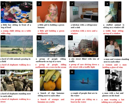
Figure 2: Quality examples of our best model (red) compared with the attention model trained under XENT loss (black).

distribution become bigger because our method encourages the action with a higher future reward being sampled more frequently by the model when training.

Qualitative Analysis

Here we provide some quality examples of our captioning model shown in Figure 2. The sentences in black are gener-ated by the pretrained attention model under the XENT loss. And the sentences in red are generated by our best model trained under the RL loss based on the pretrained attention model. So we can sense the improvement by the reinforce-ment learning intuitively by analysing the captions generat-ed by the two models. In general, the RL model can gener-ate more descriptive captions than the base attention model. Specifically, in Figure 2, for the top four images, the base attention cannot recognize some objects in the image cor-rectly. An example can be found in image 2 where the tooth-brush is mistaken as a banana by the base model, whereas the RL model correctly describes it. For the middle four images, the RL model can express the visual content in more detail and descriptively, for instance in image 7, the RL model can “see” the traffic light and “infer” that the cars are driving on the street, while the base model just recognizes the city

street and the traffic. For the bottom four images, the RL model can organize the language better matching the habit of human cognition than the base attention model. Taking image 12 as an example, this image shows us a scene that a man is talking on the cell phone. The RL model describes the scene correctly while the base attention model does not, though its description of the man is not completely wrong.

Conclusion

References

Chen, L.; Zhang, H.; Xiao, J.; Nie, L.; Shao, J.; and Chua, T.-S. 2017a. Sca-cnn: Spatial and channel-wise attention in convolutional networks for image captioning. InIEEE

Conference on Computer Vision and Pattern Recognition.

Chen, L.; Zhang, H.; Xiao, J.; Nie, L.; Shao, J.; and Chua, T.-S. 2017b. Sca-cnn: Spatial and channel-wise attention in convolutional networks for image captioning.CVPR. Chen, M.; Ding, G.; Zhao, S.; Chen, H.; Liu, Q.; and Han, J. 2017c. Reference based lstm for image captioning. AAAI. Cho, K.; Van Merri¨enboer, B.; G¨ulc¸ehre, C¸ .; Bahdanau, D.; Bougares, F.; Schwenk, H.; and Bengio, Y. 2014. Learning phrase representations using rnn encoder-decoder for statis-tical machine translation. InEMNLP, 1724–1734.

Devlin, J.; Gupta, S.; Girshick, R.; Mitchell, M.; and Zit-nick, C. L. 2015. Exploring nearest neighbor approaches for image captioning. arXiv preprint arXiv:1505.04467. Elliott, D., and Keller, F. 2013. Image description using visual dependency representations. InEMNLP, 1292–1302.

Fang, H.; Gupta, S.; Iandola, F.; Srivastava, R. K.; Deng, L.; Doll´ar, P.; Gao, J.; He, X.; Mitchell, M.; Platt, J. C.; et al. 2015. From captions to visual concepts and back. InCVPR, 1473–1482.

Farhadi, A.; Hejrati, M.; Sadeghi, M. A.; Young, P.; Rashtchian, C.; Hockenmaier, J.; and Forsyth, D. 2010. Ev-ery picture tells a story: Generating sentences from images. InECCV, 15–29.

Gong, Y.; Wang, L.; Hodosh, M.; Hockenmaier, J.; and Lazebnik, S. 2014. Improving image-sentence embeddings using large weakly annotated photo collections. InECCV, 529–545.

He, K.; Zhang, X.; Ren, S.; and Sun, J. 2016. Deep residual learning for image recognition.CVPR00:770–778.

Hochreiter, S., and Schmidhuber, J. 1997. Long short-term memory.Neural Computation9(8):1735–1780.

Jia, X.; Gavves, E.; Fernando, B.; and Tuytelaars, T. 2015. Guiding the long-short term memory model for image cap-tion generacap-tion. InICCV, 2407–2415.

Jin, J.; Fu, K.; Cui, R.; Sha, F.; and Zhang, C. 2015. Align-ing where to see and what to tell: image caption with region-based attention and scene factorization. arXiv preprint

arX-iv:1506.06272.

Kulkarni, G.; Premraj, V.; Dhar, S.; Li, S.; Choi, Y.; Berg, A. C.; and Berg, T. L. 2011. Baby talk: Understanding and generating simple image descriptions. InCVPR, 1601–1608.

Lin, T. Y.; Maire, M.; Belongie, S.; Hays, J.; Perona, P.; Ra-manan, D.; Dollr, P.; and Zitnick, C. L. 2014. Microsoft coco: Common objects in context. InECCV, 740–755.

Liu, S.; Zhu, Z.; Ye, N.; Guadarrama, S.; and Murphy, K. 2016. Optimization of image description metrics using pol-icy gradient methods.arXiv preprint arXiv:1612.00370. Lu, J.; Xiong, C.; Parikh, D.; and Socher, R. 2017. Knowing when to look: Adaptive attention via a visual sentinel for image captioning.CVPR.

Mao, J.; Xu, W.; Yang, Y.; Wang, J.; and Yuille, A. L. 2015. Deep captioning with multimodal recurrent neural networks (m-rnn). InICLR.

Ranzato, M.; Chopra, S.; Auli, M.; and Zaremba, W. 2015. Sequence level training with recurrent neural networks.

I-CLR.

Rennie, S. J.; Marcheret, E.; Mroueh, Y.; Ross, J.; and Goel, V. 2017. Self-critical sequence training for image caption-ing.CVPR.

Schwenk, H. 2012. Continuous space translation models for phrase-based statistical machine translation. In COLING, 1071–1080.

Sutton, R. S. 1988. Learning to predict by the methods of temporal differences.Mach. Learn.3(1):9–44.

Vinyals, O.; Toshev, A.; Bengio, S.; and Erhan, D. 2015. Show and tell: A neural image caption generator. InCVPR, 3156–3164.

Williams, R. J. 1992. Simple statistical gradient-following algorithms for connectionist reinforcement learning.

Ma-chine learning8(3-4):229–256.

Wu, Z. Y. Y. Y. Y., and Cohen, R. S. W. W. 2016. Encode, re-view, and decode: Reviewer module for caption generation.

NIPS.

Xu, K.; Ba, J.; Kiros, R.; Cho, K.; Courville, A.; Salakhudi-nov, R.; Zemel, R.; and Bengio, Y. 2015. Show, attend and tell: Neural image caption generation with visual attention. InICML, 2048–2057.

Yao, T.; Pan, Y.; Li, Y.; Qiu, Z.; and Mei, T. 2016. Boost-ing image captionBoost-ing with attributes. arXiv preprint

arX-iv:1611.01646.

You, Q.; Jin, H.; Wang, Z.; Fang, C.; and Luo, J. 2016. Image captioning with semantic attention. InCVPR, 4651– 4659.

Zhao, S.; Yao, H.; Gao, Y.; Ji, R.; and Ding, G. 2017. Contin-uous probability distribution prediction of image emotions via multitask shared sparse regression. IEEE Transactions