Autonomous Data-driven Clustering for Live Data
Stream
Xiaowei Gu and Plamen P. Angelov
Data Science Group, School of Computing and Communications, Lancaster University,
Lancaster, LA1 4WA, UK. E-mail: [email protected]
Abstract— In this paper, a novel autonomous data-driven clustering approach, called AD_clustering, is presented for live data streams processing. This newly proposed algorithm is a fully unsupervised approach and entirely based on the data samples and their ensemble properties, in the sense that there is no need for user-predefined or problem-specific assumptions and parameters, which is a problem most of the current clustering approaches suffer from. Moreover, the proposed approach
automatically evolves its structure according to the
experimentally observable streaming data and is able to recursively update its self-defined parameters using only the current data sample, meanwhile, discards all the previous data samples. Experimental results based on benchmark datasets exhibit the higher performance of the proposed fully autonomous approach compared with the comparative approaches with user- and problem- specific parameters to be predefined. This new clustering algorithm is a promising tool for further applications in the field of real-time streaming data analytics.
Keywords— fully unsupervised clustering; live data streams; ensemble properties; recursive update; streaming data analytics
I. INTRODUCTION
Due to the fast progress of information and hardware technologies, in the past few years, astronomical amount of streaming data is being generated from various aspects of human societies and daily lives, such as network flows, sensor data and website traffic. Analyzing these data is becoming increasingly important because of the valuable information with the data streams. Facing the potential and challenge at the same time, data analytics is now a rapidly growing field involving the efforts of researchers and scholars from all over the world.
Currently, clustering algorithms require a number of assumptions and parameters to be known in advance [1-9], for instances, number of clusters in k-means clustering algorithm [1], the kernel size in mean shift clustering algorithm [2], which usually are impractical for users to decide in reality. In addition, most of the well-known clustering algorithms [1-5] as well as many recently proposed clustering algorithms [8, 10] are restricted to offline data processing and not applicable to the live data streams with potential changes of data patterns [11, 12]. In order to handle the huge amount of data samples continuously arriving with the data streams, the clustering algorithm needs to be memory- and computation- efficient [13]. The system structure of the clustering algorithm also
should have the ability to evolve, which means the system structure will be changing all the time to follow the shifts and drifts of the data streams [11].
In this paper, a novel autonomous data-driven clustering algorithm, named AD_clustering, is proposed for live data streams processing. This algorithm is entirely based on the data and their mutual distribution in the data space. No predefined specific parameter or assumption is needed in AD_clustering
clustering. The proposed approach starts “from scratch”, self-decides its structure as well as all parameters according to the density and the ensemble features of the data samples in the live data streams. Once the structure and parameters are defined, the algorithm keeps re-adjusting them to follow the time-varying data pattern.
In addition, the proposed approach sequentially learns from the current data sample and automatically discards all the previous data samples. Therefore, all the parameters of the proposed approach are updated recursively and only the meta-information is stored in memory, which ensures AD_clustering
the advantages of computation-and memory-efficiency.
This remainder of this paper is organized as follows. Section II introduces the theoretical basis of the proposed algorithm. The proposed algorithm is described in section III and the summary is given in section IV. Section V presents the numerical experiments and section VI concludes the paper.
II. THEORETICAL BASIS
In this section, the theoretical basis of the proposed
AD_clustering approach will be introduced. The main
quantities representing ensemble properties of the data samples of the live data stream will be firstly introduced followed by their corresponding recursive calculation expressions of these quantities. The well-known Chebyshev inequality will be briefly recalled in the end of this section.
A. Main Quantities
First of all, considering the real Hilbert space Rd, we assume the live data stream with continuous arrival of new data samples is denoted as
x1,x2,x3,...,xk,...
, where the subscripts indicate the time instance at which each data sample arrives and each data sample has d dimensions.1) Cumulative proximity
Cumulative proximity is used to measure how close/similar of a particular data sample is to all other existing data samples [14].
The centrality of the data sample xi is calculated as:
d i kk
j
j i i
k ( , ) 1,2,...,
1 2
x x x (1)
where d(xi,xj)denotes the distance between the two data samples xi and xj. The distance can be of Euclidean, Mahalanobis type and other metrics based on cosine [15]. In this paper, we only use the most representative Euclidean distance for derivation, namely d(xi,xj) xi xj .
2) Standardized eccentricity
Standardized eccentricity is directly derived from eccentricity introduced in [14] as a measure that represents the association of the data point with the tail of the distribution and the property of being an outlier/anomaly. The expression of standard eccentricity of the data sample xi is as follows:
i kk k k j k v v j k v v i k j j k i k i
k 1,2,...,
2 2 1 1 2 1 2 1
x x x x x x x (2)
Notice that :
kk i i k 2 1
x .3) Density
Density is the inverse of the standardized eccentricity expressed as follows,i1,2,...,k[14]:
k v v i k j k v v j i k k j j k i k i k k k D 1 2 1 1 2 1 2 2 1 x x x x x x x x (3)
B. Recursive Expressions of Calculation
The memory- and calculation-efficiencies of the algorithm for online data stream processing mainly rely on the recursive expressions of calculation of the main quantities used in the algorithm.
The recursive expression of xi’s cumulative proximity is
[15]:
2 2
k k k i i
k x k x μ X μ
(4)
where μk 1μk11xk μ1x1 k
k k
(5)
1 11 x 2 X1 x1 2 k
X k k
Xk k k (6)
The sum of the cumulative proximity of all the existing data samples can also be updated recursively using (7) [15]:
k
kk i i k k i i
k x x x
2 1 1 1 1
(7)Therefore, by utilizing (4) and (7), the online recursive expressions of standardized eccentricity and density are as follows [15]:
2 2 2 2 2 1 1 1 2 2 1 1 1 2 2 2 2 2 2 2 k k k i k k k k k i i k i k k k k k k i i k k k k i i k X k X k D X k X k μ μ x μ μ x x x μ μ x x μ μ x x (8)C. Chebyshev Inequality
The well-known Chebyshev inequality states that, in any
probability distribution, no more than 12
n of the values of the
distribution can be n standard deviations away from the mean [16]. For Euclidean type of distance, the Chebyshev inequality has the following form:
22 2 2 1 1 n n
P xi μk k (9) where k is the standard deviation of all the existing data samples to their mean, and there is k2 Xk μk 2. In this approach, the Chebyshev inequality will be used to decide the radius of the cluster.
III. THE PROPOSED AD_CUSTERING ALGORITHM
AD_clustering is a novel online algorithm based entirely on the ensemble properties of the data samples. The proposed algorithm does not require any user- or problem- specific assumption or parameters to be predefined. Only a few meta-information is needed to be kept in memory and all the parameters can be updated recursively, which makes the algorithm efficient and suitable for live data streams.
The global meta-parameters need to be kept in memory are as follows:
1) Mean of the data samples: μk.
2) Mean of scalar product of the data samples: Xk.
3) The sum of the cumulative proximity of all the existing
data samples:
k i i k 1 x .4) Number of the existing clusters: Nk.
1) The support of the cluster (number of members of the cluster):Sj.
2) Center of the cluster (mean of all the data samples in the
cluster):
j S i i j j jS 1 ,
1
x
c , where xj,idenotes the ith data
sample of the jthcluster.
3) The mean of square of the data samples belonging to the
cluster:
j S i i j j j S L 1 2 , 1 x .
There is no need to keep the radii of the clusters because the radii can be obtained directly from cjand Ljusing the Chebyshev inequality given in section II:
k j j j r j
j n L j N
r x, c c 2 1,2,, (10) where xj,re is the assumed farthest member for the jthcluster.
Here n2 is used in our algorithm because it ensures the cluster to have enough tolerance to normal deviations but still be sensitive to abnormal data samples.
In rest of this section, we will demonstrate the three stages of the proposed algorithm.
A. Global Update Stage
For each new data sample, the first stage of the proposed algorithm focuses on the updating of global parameters and finding out the cluster that the new coming data sample is associated to.
At each time a new data sample denoted as xk1 comes, the global parameters μkand Xkare updated firstly to μk1and
1
k
X using (5) and (6) respectively.
Then, the cumulative proximity k1
xk1 of xk1is calculated using (4) and the sum of cumulative proximity of allexisting data samples
k i i k 1 x is updated using (7). With the
new k1
xk1 and
1 1 1 k i i k x , xk1’s density Dk1
xk1 isobtained using (8).
The densities of the centers of all the existing clusters are also needed to be updated to help decide whether there is new cluster appearing:
2 1 1 2 1 2 1 1 1 1 12 j k k k
k i i k j k X k D μ μ c x c (11)
where j1,2,...,Nk; Nk is the number of existing clusters at the time instance k; cjis the center of the jth existing cluster.
After all the global parameters have been updated, we come to the second stage of the proposed approach.
B. Local Update Stage
At the beginning of this stage, we need to check Condition A [17]:
Condition A:
1
min max 1 1 1 1 1 1 1 1 1 k k j k N j k k j k N j k k N N THEN D D OR D D IF k k c x c x (12)
If Condition A is satisfied, the new data sample is associated with a new cluster, Nk1Nk1. xk1 is set to be the original center
1
k N
c of the new cluster and other local
parameters are set to be 1
1
k N
S and 1 2
1
k
Nk
L x .
On the contrary, if Condition A is not satisfied, xk1 is a potential member of one of the existing clusters and
k
k N
N1 . The cluster that xk1 possibly belongs to is decided by the following equation:
1 1
min
arg
N j k
j k
label
Cluster c x (13)
After the label of the possible cluster that xk1 could be assigned is obtained, it is necessary to check whether xk1 is within the radius of influence of the cluster. Denoting the center of the selected cluster as cv, if the support of the cluster
1
v
S , we assign xk1 to the cluster directly and update the corresponding parameters as follows:
1 _new v
v S
S (14a)
2 1 _
v k new
v
x c
c (14b)
2 1 _ 2 1 2 1 v k
new
v L
L x (14c)
while, if Sv1, Condition B is needed to be checked:
Condition B:
v k1 rv
THEN
Nk1Nk1
IF c x (15)
where rv n Lv cv 2 .
Fig. 1 Illustration of Condition C
Fig. 2 Illustration of Condition D
In contrast, when Condition B is not met, xk1 is a formal member of the existing cluster with center cv. The local parameters of this cluster are updated recursively:
1 _new v
v S
S (16a)
1 _ _ _ 1 k new v v new v v new v S S S x c
c (16b)
2 1 _ _ _ 1 k new v v new v v new v S L S S
L x (16c)
For other clusters that do not take in new member at the current time instance, their local parameters are kept as the same.
C. Adjustment Stage
In this stage, all the existing clusters will be examined and adjusted to avoid overlap.
Condition C is executed first.
Condition C:
1
... ) , max( ) , max( k k i l i l i j i j i N N AND Split THEN AND r r AND r r IF c c c c c (17)
If the ith cluster meets Condition C, it means that more than two other clusters have covered this cluster. In this case, the ith
cluster should be split according to the following rules:
il l new l ij j new
j S s S S s
S _ _ (18a)
i new j ij j new j j new j i new l il v new l l new l S s S S S s S S c c c c c c _ _ _ _ _ _ (18b) 2 _ _ _ 2 _ _ _ i new l il l new l l new l i new j ij j new j j new j S s L S S L S s L S S L c c (18c)
where Si sijsil; (19a)
i l i j i l i il i l i j i j i ij S Ro s S Ro s c c c c c c c c c c c c
; (19b)
Ro denotes the operation - round to the nearest integer.
Then, we check Condition D:
Condition D:
1
) , max( k k j i j i j i N N AND and Merge THEN r r IF c c c c (20)
If the ith and the jth cluster satisfy Condition D, the two clusters are very close to each other. We should merge them together according to the following rules:
j i new
i S S
S_ (21a)
j new i j i new i i new i S S S S c c c _ _
_ (21b)
j new i j i new i i new i L S S L S S L _ _
_ (21c)
Here, the new ith cluster becomes a combination of the old
ith cluster and jth cluster.
After Condition C and Condition D are checked, the adjustment stage is finished, and the algorithm is ready for the next data sample.
In order to ensure the most comprehensive output, once a cluster is formed, the proposed algorithm will keep its meta-parameters in memory unless it is split or merged with others. Nonetheless, all the clusters will automatically be divided into three classes according to their support for easier analysis of the result.
For the clusters with support smaller than 3, they are recognized as abnormal clusters. With the shift and drift of the data pattern [11], these clusters will possibly grow into minor clusters or major clusters later. Despite of their potential, at the time instance that output of the algorithm is carried out, they are meaningless, and can be viewed as noise.
2) Major clusters
The clusters, which have supports above threshold Sthreshold, can be viewed as major clusters. Namely, they are the most representative and important clusters in the data streams. The major clusters are the output of the AD_clustering algorithm because they represent the ensemble properties within the data samples in a relatively high degree.
The threshold Sthreshold is set to be a quarter of the average value of the numbers of data samples allocated to “meaningful” (non-abnormal) clusters and can be expressed as:
k N
i i threshold
N S S
k
1 4 1
(22)
where Nk is the number of clusters with supports Sj 2 ( j1,2,...,Nk); {Si}is the collection of clusters’ supports that satisfy Sj 2 (j1,2,...,Nk).
3) Minor clusters
The clusters, which have the supports below threshold
threshold
S , are recognized as minor clusters. Minor clusters are less important clusters in the clustering results at the time instance that output of the algorithm is carried out. If new data samples continue to arrive, they have potential to be major clusters due to the possible shift/drift of data pattern [11]. Minor clusters serve as the optional output if users want to see a more detailed result.
IV. ALGORITHM SUMMARY
The overall algorithm process is summarized in this section presented in the form of pseudo-code.
AD_clustering Algorithm
While the data samplexk is available (or until not interrupted)
I. If (k1) Then
1.μ1x1; 2.X1 x1 2; 3.
01
1
1
ii
x
;
4.N11;
5.c1x1; 6.S11; 7.L1 x1 2; II. Else
1. Update μkandXk using eq. (5) and eq. (6);
2. Calculate k
xk using eq. (4);3. Update
ki i k
1 x
using eq. (7);
4. Calculate Dk
xk using eq. (8);5. Update the Dk
cj (j1,2,...,Nk) using eq. (11);6. If (Condition A is met) Then
a. N k
k x
c 1 ;
b.SNk11; c. N 1 k 2
k
L x ;
d.Nk Nk1; 7. Else
a. Use eq. (13) to find the possible cluster v for
k
x ;
b. If (Sv1) Then
i. Update Sv, cv Lvusing eq. (14); c. Else
i. If (Condition B is met) Then
*. Update Sv, cv Lvusing eq. (14); ii. Else
*. N k
k x
c 1 ;
*. 11
k N
S ;
*. N 1 k 2
k
L x ;
*.NkNk1; iii. End If
d. End If
8. End If
9. While there are existing clusters meeting Condition C)
a. Split the clusters using eq. (18)-(19); 10. End While
11. While there are existing clusters meeting Condition D)
a. Merge the clusters using eq. (21); 12. End While
III. End If End While
V. NUMERICAL EXPERIMENTS
In this section, numerical experiments with several benchmark datasets are conducted to test the performance of the newly proposed AD_clustering algorithm.
A. Benchmark Datasets
Seven benchmark datasets are used in the experiments with Euclidean type of distance:
1) Fisher Iris Dataset [18]:
2) Climate Dataset [19]:
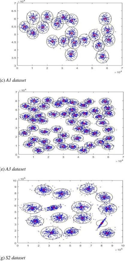
3) A1 Dataset [20];
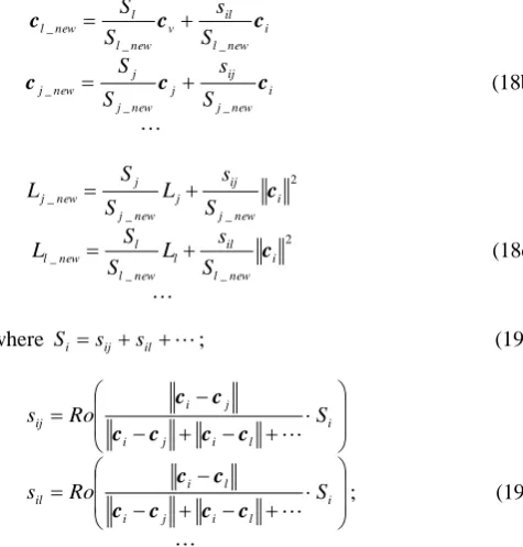
TABEL II (a).EXPERIMENTAL RESULTS
UIa Data set
Measures
Nfinal Nmaj Kmaj Smax Smin texe
AD b
FI
9 3 137 60 32 0.11
MS c
0.1 145 1 3 3 3 0.04
0.5 20 9 137 36 4 0.02 1 2 2 150 100 50 0.02
EC d 0.05 4 3 149 70 18 0.02
0.5 4 2 139 70 69 0.02 AD
C
3 2 936 475 461 0.32
MS
1 920 1 3 3 3 0.82
5 98 11 775 334 9 0.13 10 8 2 929 494 435 0.06
EC
10 8 6 908 309 49 0.10 100 5 5 938 411 58 0.10
a.
User Input; b.
AD_clustering Algorithm; c.
Mean Shift Algorithm; d.
[image:6.595.303.569.62.596.2]eClustering Algorithm. TABLE I. BENCHMARK DATASET DESCRIPTION
Data set
Details Number of
Data Samples
Number of clusters
Number of Attributes
Maximum Cluster
size
Minimum Cluster
size
FI a 150 3 4 50 50
C b 938 2 6 479 459
A1 3000 20 2 150 150
A2 5250 35 2 150 150
A3 7500 50 2 150 150
S1 5000 15 2 350 300
S2 5000 15 2 350 300
a.
Fish Iris; b. Climate.
TABEL II (b).EXPERIMENTAL RESULTS
UI Data set
Measures
Nfinal Nmaj Kmaj Smax Smin texe
AD
A1
27 20 2989 154 143 8.39
MS
100 2756 23 70 4 3 9.65
1000 236 132 2783 100 5 0.27 5000 17 17 3000 324 139 0.04
EC
10 3 3 3000 2274 340 0.28 1000 1 1 3000 3000 3000 0.25 AD
A2
53 35 5213 160 140 39.99
MS
100 4791 45 144 5 3 44.68 1000 408 217 4854 101 5 0.7 5000 28 28 5250 393 75 0.07
EC
10 3 2 4909 3774 1135 0.50 1000 1 1 5250 5250 5250 0.43 AD
A3
71 50 7456 160 140 111.74
MS
100 6851 59 185 5 3 114.34 1000 558 296 7000 131 5 1.24 5000 41 40 7477 417 79 0.10
EC
10 3 2 7159 4269 2890 0.72 1000 1 1 7500 7500 7500 0.61 AD
S1
42 15 4763 349 218 35.31
MS
500 4787 33 124 7 3 39.51 5000 2038 466 3030 166 3 7.09 25000 111 21 4678 347 21 0.28
EC
10 2 2 5000 2737 2263 0.47 1000 2 2 5000 2737 2263 0.47 AD
S2
31 15 4849 360 240 20.55
MS
500 4831 23 91 10 3 39.62 5000 2460 410 2514 94 3 9.98 40000 196 57 4528 327 9 0.33
EC
10 2 2 5000 3685 1315 0.46 1000 2 2 5000 3685 1315 0.47 5) A3 Dataset [20];
6) S1 Dataset [20];
7) S2 Dataset [20];
Details of the seven datasets are given in Table I. Although, these datasets were primarily for offline processing, they are transformed into live data streams according to the rule that at each time instance only one data sample is used as the input to the clustering approach.
B. Results
Due to the fact that the proposed AD_clustering approach is for live data streams, the algorithm will not keep the members of the existing clusters in the memory because each time after the newly coming data sample is processed, it is discarded. Nonetheless, we still can measure the performance of the algorithm by using the standard measures as detailed below:
1) Number of clusters generated from all the data, Nfinal;
2) The number of major clusters, Nmaj;
3) The number of data samples in major clusters, Kmaj;
4) Maximum support of the major clusters, Smax;
5) Minimum support of the major clusters, Smin;
[image:6.595.33.290.479.707.2]
(b) Climate dataset (c) A1 dataset
(d) A2 dataset (e) A3 dataset
[image:7.595.310.521.261.695.2]
(f) S1 dataset (g) S2 dataset Fig. 3 Experimental results
(a) Fisher iris dataset The detailed experimental results are depicted in Table II. The 2D figures of the clustering results are additionally depicted in Fig. 3.
For further discussion of the performance, the proposed
AD_clustering algorithm is compared with two well-known clustering algorithms: mean shift clustering algorithm (offline) [2] and eClustering algorithm (online) [7]. To ensure the effectiveness of the comparison, we additionally apply the same rule measuring the importance of clusters described in Section III to the experimental results of the comparative algorithms
Because this paper is focused on a new method for live data streams analytics, the requirement of user inputs is also taken into consideration. For mean shift clustering algorithm, kernel size is the parameter needed to be predefined and ‘for
eClustering algorithm, user needs to predefine the initial radius.
As we can see clearly from Table II, the mean shift
proper user input, namely kernel size, which is often impractical in real cases because of the lack of prior
knowledge. eClustering algorithm is the fastest and more stable than mean shift clustering algorithm. However, its accuracy is not as high as that of AD_clustering.
Comparatively, the clustering results of the newly proposed online AD_clustering algorithm are supreme compared with the other well-known clustering algorithms. Without the need of prior knowledge or pre-defined parameters from users,
AD_clustering algorithm is entirely driven by the data streams and exhibits high purity results. Despite of the fact that the proposed algorithm costs more time that the two comparative algorithms, it is acceptable due to its excellent performance and the feature of being totally free of user inputs.
VI.CONCLUSION
A fully autonomous unsupervised clustering algorithm called AD_clustering is introduced in this paper. This newly proposed clustering algorithm is entirely free of any kind of user- and problem- specific restrictive assumptions and parameters. The algorithm is completely based on the data samples and their mutual distributions and is able to self-define and re-adjust its system structure as well as parameters. The recursive update of the parameters ensure the proposed algorithm to be calculation-efficient, and update parameters only based on the current data sample also give AD_clustering
algorithm the advantage of memory-efficiency, which make this approach extremely suitable for online data stream processing. This newly proposed algorithm is a solid basis and promising tool for the area of streaming data analytics.
In the future, we intend to conduct the research on the performance of this algorithm using different distances and dissimilarities including Mahalanobis type and other metrics based on cosine, and will be further applied to other fields like natural language processing.
REFERENCES
[1] J. MacQueen, “Some methods for classification and analysis of multi-variate observations”, in Porceedings of the Fifth Berkeley Synposium on Mathematical Statistics and Probability, Volue 1: Statistics, Berkeley, 1967, pp. 281-297.
[2] K. Fukunaga and L. Hostetler, “The estimation of the gradient of a density function, with applications in pattern recognition”, IEEE Transactions on Information Theory,1975, vol. 21(1), pp. 32-40. [3] Yager, R. and D. Filev, “Generation of fuzzy rules by mountain
clustering”, Journal of Intelligent & Fuzzy Systems, 1994, vol. 2(3), pp. 209-219.
[4] Chiu, S.L., “Fuzzy model identification based on cluster estimation”. Journal of Intelligent & Fuzzy Systems, 1994, vol.2(3), pp. 1064-1246. [5] M. Ester, H. P. Kriegel, J. Sander, and X. Xu, “A density-based
algorithm for discovering clusters in large spatial databases with noise”, in 2nd International Conference on Knowledge Discovery and Data Mining. 1996. Portland, Oregan, vol. 96(34), pp. 226-231.
[6] J. Csirik, L. Epstein, C. Imreh, and A. Levin, " Online clustering with variable sized clusters", Algorithmica, 2013, vol.65(2), pp.251-27. [7] P. Angelov, "An approach for fuzzy rule-base adaptation using on-line
clustering", International Journal of Approximate Reasoning, 2004, vol.35(3), pp. 275-289.
[8] R. Hyde and P. Angelov, "A fully autonomous Data Density based Clustering technique", 2014 IEEE Symposium on Evolving and Autonomous Learning Systems (EALS), 2014, Orlando, pp.116-123. [9] C. Wang, J. Lai, D. Huang and W. Zheng, "SVStream: A support
vector-based algorithm for clustering data streams", IEEE Transactions on Knowledge and Data Engineering, 2013, vol.25(6), pp.1410-1424. [10] P. Angelov, X. Gu, G. G. Gutierez, J. A. Iglesias and A. S. de Miguel,
“Autonomous data density based clustering method”, in IEEE World Congress on Computational Intelligence, 24-29 July 2016, Vancouver, Canada, in press.
[11] E. Lughofer and P. Angelov, "Handling drifts and shifts in on-line data streams with evolving fuzzy systems", Applied Soft Computing Journal, 2011, vol.11(2), pp.2057-2068
[12] P. Angelov, ‘Outside the Box: An Alternative Data Analytics Framework’. Journal of Automation, Mobile Robotics and Intelligent Systems, 2014, vol. 8(2), pp. 53-59.
[13] J. Silva, E. Faria, R. Barros, E. Hruschka, A. de Carvalho and J.Gama, "Data stream clustering: A survey", ACM Computing Surveys, 2013, vol.46(1), p.13.
[14] P. Angelov, X. Gu, J. Principe and D. Kangin, “Empirical data analysis: A new tool for data analytics”, unpublished.
[15] P. Angelov, X. Gu and D. Kangin, “TEDA: typicality based empirical data analysis”, unpublished.
[16] J. Saw, M. Yang, and T. Mo, "Chebyshev inequality with estimated mean and variance", The American Statistician, 1984, vol.38(2), pp.130-132
[17] P. Angleov, Autonomous Learning Systems from Data Stream to Knowledge in Real Time. West Sussex, United Kingdom: John Wiley & Sons, Ltd., 2012.