Joint Analysis of Binomial and Continuous Traits with a Recursive Model: A Case Study Using Mortality and Litter Size of Pigs

(1)

INVESTIGATION

Joint Analysis of Binomial and Continuous Traits

with a Recursive Model: A Case Study Using

Mortality and Litter Size of Pigs

Luis Varona* and Daniel Sorensen†,1

*Departamento de Anatomía, Embriología y Genética Animal, Facultad de Veterinaria, Universidad de Zaragoza, E-50013, Spain, and†Department of Molecular Biology and Genetics, Aarhus University, PB 50, DK-8830 Tjele, Denmark

ABSTRACTThis work presents a model for the joint analysis of a binomial and a Gaussian trait using a recursive parametrization that leads to a computationally efﬁcient implementation. The model is illustrated in an analysis of mortality and litter size in two breeds of Danish pigs, Landrace and Yorkshire. Available evidence suggests that mortality of piglets increased partly as a result of successful selection for total number of piglets born. In recent years there has been a need to decrease the incidence of mortality in pig-breeding programs. We report estimates of genetic variation at the level of the logit of the probability of mortality and quantify how it is affected by the size of the litter. Several models for mortality are considered and the bestﬁts are obtained by postulating linear and cubic relationships between the logit of the probability of mortality and litter size, for Landrace and Yorkshire, respectively. An interpretation of how the presence of genetic variation affects the probability of mortality in the population is provided and we discuss and quantify the prospects of selecting for reduced mortality, without affecting litter size.

M

IXED linear models (Henderson 1984) are broadly used in livestock and plant breeding and play an im-portant role in evolutionary and theoretical quantitative ge-netics (Lande 1979; Cheverud 1984; Walsh 2003). The classical approach for a multiple-trait analysis is to use mod-els posing that the nature of the correlation between response variables (phenotypes) is due to linear associations between unobservables, such as additive genetic values or nongenetic sources, like permanent or temporary environmental effects. Structural equation models represent an extension of the standard linear model to account for links (feedback and/or recursiveness) involving either the phenotypes directly or latent variables; they are well established in econometrics and sociology (Goldberger 1972; Jöreskog 1973; Duncan 1975). These models were discussed in the early genetics literature by Wright (1921) but this work has not received much atten-tion in quantitative genetics. Xionget al.(2004) proposed the

use of structural equation models for modeling and identifying genetic networks. In a quantitative genetics context, Gianola and Sorensen (2004) studied the consequences of the existence of simultaneous and recursive relationships between phenotypes on genetic parameters and presented statistical methods for in-ference. An application to study the relationship between somatic cell score and milk yield in goats is in de los Camposet al.(2006). Varonaet al.(2007) present a recursive model for the joint anal-ysis of litter size and average litter weight in Danish pigs. These studies were concerned with normally distributed traits. Here the methodology is developed further for the joint analysis of a bi-nomial and a continuous trait and it is shown that a computation-ally simple implementation can be arrived at by appropriate choice of the recursive speciﬁcation. The method is illustrated using mortality and litter size in two breeds of Danish pigs.

Litter size is basically determined by ovulation rate and embryo mortality (Blasco et al.1995); these processes take place mainly at the early stages of gestation. Piglet weight at birth is determined mostly by growth in late gestation and is importantly related to piglet survival. It is then reasonable to postulate a one-way causal path establishing an effect of litter size on piglet mortality. This speciﬁcation deﬁnes a recursive two-trait system. On the other hand, simultaneity occurs when trait 1 affects trait 2 and vice versa.

Manuscript received December 16, 2013; accepted for publication January 7, 2014; published Early Online January 10, 2014.

Supporting information is available online athttp://www.genetics.org/lookup/suppl/ doi:10.1534/genetics.113.159475/-/DC1.

1_{Corresponding author: Department of Molecular Biology and Genetics, Aarhus}

(2)

Litter size has been under selection in the Danish pig-breeding program since the early nineties and resulted in considerable increase in total number born and also in the proportion of stillborn piglets (Sorensenet al.2000; Suet al. 2007). Sorensenet al.(2000) report an increase in the ob-served proportion of piglets born dead at higher-litter-size values. This has raised a number ethical and economic con-cerns and has led to measures designed to reduce mortality. A recently implemented approach in the Danish pig-breeding program is based on changing the emphasis of selection from total number born to total number of piglets alive 5 days after farrowing (Su et al.2007). Despite the fact that this selection strategy is not addressing the problem of mor-tality directly, it seems to have had a beneﬁcial effect on both litter size and mortality (Nielsenet al.2013).

A number of studies have reported genetic variation for mortality with heritabilities ranging from 0.03 to 0.17. These studies have assumed normality of the sampling model for mortality (e.g., Van Arendonket al.1996), based inferences on a variety of threshold models (e.g., Roehe and Kalm 2000; Arango et al.2006), or implemented mixed models for count data (Varona and Sorensen 2010). Mortality data, regarded as a trait of the mother, show typically a large proportion of “zeros”(many litters do not have stillborn piglets). The study of Varona and Sorensen (2010) included a variety of models that accounted for this feature of the data and concluded that the best ﬁt was achieved with a hierarchical binomial logit mixed model. In this work we extend this model in two direc-tions. First, the probability of mortality is assumed to be a func-tion of the total number of piglets born in the litter. This is achieved by assigning a recurrent relationship between the logit of the probability of mortality and litter size. Linear and higher-order functions of litter size are investigated, and the quality of

ﬁt of the models is studied. The second extension allows for a joint analysis of mortality and litter size. The recursive param-eterization implemented has the attractive feature that the joint posterior distribution of the two traits factorizes into two in-dependent posterior distributions, one for each trait, whereby the computational burden of implementation is reduced.

The article is organized as follows.Material and Methods introduces the models, including the prior and posterior dis-tributions, the method used to compare the models, and a brief description of the data. This is followed by Results, where the focus is on mortality but results for litter size are brieﬂy reported. A Discussion comprises theﬁnal section of the paper and theAppendixsketches technical details regard-ing the model and the Markov chain Monte Carlo algorithm.

Material and Methods

Model and prior distributions

Total number of dead piglets at birth (called mortality hereinafter, treated as a trait of the mother) and total number of piglets born (called litter size hereinafter, treated as a trait of the mother) are analyzed jointly using a model that exploits the

factorization of their joint distribution. The conditional binomial model for mortality in litteri,Yi, given litter size in litteri,tiis

fðYi¼yijti;fiÞ ¼

ti

yi

fyi

ið12fiÞti2yi; Yi¼0;1;. . .;ti;

(1) wherefiis the probability that a piglet dies (referred to as

the probability of mortality hereinafter) in litter i, which is assumed to vary over the observations as an inverse logistic deterministic function of unknown parameters. Thus, the linear structure of the logit offiis assumed to be equal to

logit fi¼x9iayþz9iu~yþw9i~pyþgjðtiÞ; (2)

wherex9i,z9i, andw9iare vectors of observed incidence

matri-cesX,Z, andW,ayis a vector of systematic effect parameters

affecting mortality (herd-year and parity), ~uy is a vector

of residual additive genetic values affecting mortality

de-ﬁned in theAppendix,p~y is a vector of residual permanent

environmental effects affecting mortality (see also the Appendix for an explanation), and g1(t1) = l1ti (j = 1

for Model 1), g2ðtiÞ ¼l1tiþl2ti2 (j = 2 for Model 2),

g3ðtiÞ ¼l1tiþl2ti2þl3t3i (j = 3 for Model 3), where the l9s are recurrent parameters. In the case of Model 1 it is easy to see that two possible partitions are

logit fi¼x9iayþz9iu~yþw9i~pyþl1ti

¼x9iayþz9iuyþw9ipyþl1x9iatþl1eti;

where uyi¼EðuyiutiÞ þu~yi and pyi ¼Eðpyi

j

ptiÞ þ~pyi (see Appendix) represent draws from the marginal distributions of additive genetic values and permanent environmental effects affecting mortality.

Given vectors of systematic effectsat(herd-year and parity),

of additive genetic valuesutand of permanent environmental

effectspt, litter size records are conditionally independent and

assumed to follow the Gaussian process tijat;ut;pt N

x9iatþz9iutþw9ipt;s2et

: (3)

In theAppendixit is shown that the structure ofð~pyi;ptiÞis

~ pyi;pti

N

" 0 0

; s

2

~ p_y 0

0 s2pt !#

and also in theAppendixit is shown that under the recursive parameterization employed,

~ uyi;uti

N

" 0 0

; s2u~y 0 0 s2ut

!# :

The covariance matrix of the joint distribution of the vectors ~

uyandutisG5A, whereG¼diagðs2_~uy;s 2

(3)

p

euy;utjA;s2u_~y;s

2 ut ¼p ~ uyA;s2u_~y

p

utjA;s2ut

and similarly, p

~

py;ptjs2_~py;s

2 pt ¼p ~ pys2~py

p

ptjs2pt

:

In these expressions,Ais the additive genetic relationship ma-trix, s2

~

uy is the residual additive genetic variance for mortality (conditional variance of the additive genetic value for mortality, given the additive genetic value of liter size),s2

utis the additive genetic variance for litter size,s2

py is the variance of permanent environmental effects for mortality, ands2

pt is the variance of permanent environmental effects for litter size. The phenotypic variance for litter size iss2

t ¼s2utþs 2 ptþs

2

et, wheres 2 et is the variance of the conditional distribution of litter size.

The variance component parameters, the recurrent param-eters, and the vectors ay and at are assigned independent

improper uniform distributionsa priori. Posterior distributions

Given the likelihood models (1) and (3) and the prior distributions of the parameters, the joint posterior distribu-tions corresponding to Model 1, say, are

p

ay;~uy;p~y;at;ut;pt;l1;s2_~uy;s

2

~ py;s

2 ut;s

2 pt;s

2 ety;t

}fyjt;ay;~uy;~py;l1

pðtjat;ut;ptÞ

3p

~ uys2_~uy

p

~ pys2_~p_y

p

utjs2ut

p

ptjs2pt

;

(4)

where y andt are vectors with elements yi and ti,

respec-tively and f

yjt;ay;~uy;p~y;l1;l2;l3

¼ Qn

i¼1

fðYi¼yijti;fiÞ

¼ Qn

i¼1

ti

yi

!

fyi

ið12fiÞti2yi;

pðtjat;ut;ptÞ¼

2ps2

et ₂n=2

exp h

2 1 2s2

etðt2XatþZutþWptÞ 9

3ðt2XatþZutþWptÞ

i :

Note that in (4), the joint posterior distribution factorizes into two independent posterior distributions, one for each trait. Model comparison

The models are compared using the pseudo-log-marginal prob-ability of the data. The pseudo-log-marginal probprob-ability of the data is a standard measure of model comparison (Gelfand 1996) and is deﬁned and computed as follows. Consider data vector y9¼ ðyi;y9₂iÞ, whereyiis theith datum, andy2iis the vector of

data with theith datum deleted. The conditional predictive dis-tribution can be interpreted as the probability of each data point given the remainder of the data and has probability density

pðyijy₂iÞ ¼

R

pðyiju;y₂iÞfðujy2iÞdu; u¼ fuigni¼1;

(5)

where u is the vector of parameters. The actual value of p(yi|y2i) is known as the conditional predictive ordinate

(CPO) for the ith observation. The pseudo-log-marginal probability of the data are given by

X

i

lnpðyijy₂iÞ: (6)

A Monte Carlo approximation of the CPO (5) for observa-tioniis given by (Gelfand 1996)

p

︹_ð

yijy₂i;MkÞ¼N

2 4XN

j¼1

1 p

yijuðijÞ;Mk

3 5

21

; (7)

where N is the number of MCMC draws, Mk is a label for

modelk, anduð_ijÞis thejth draw from the posterior ofuiunder

model k corresponding to theith observation. The so-called Log CPOs reported below are based on

X

i

ln^pðyijy₂i;MkÞ:

MCMC algorithm

The fully conditional posterior distributions associated with mortality do not all have closed forms, except for the variance

Figure 1 Raw phenotypic averages of the

(4)

componentss2

~ uyands

2

~

py, which are scaled inverted chi-square distributions and can therefore be easily updated. For the remaining parameters of the model,ay;u~y, and~py, a random

walk single-site Metropolis–Hastings algorithm was chosen as updating strategy. This required a little preliminary experi-mentation to tune the input parameters. For ~uy and~py, the

random walk proposal consisted of a draw from a uniform distribution centered at the current value, and with lower and upper bounds given by plus and minus the updated draw fromsu~y ands~py, respectively. For ay the uniform was also centered at the current value and the bounds were given by 60.15. In the case of the recursion parameters, the bounds were as follows: forl1,60.015, forl2,60.0015, and forl2, 60.00015. Theﬁnal inference was based on single chains of length 5 million (several were run with different starting values as checks and the convergence of the chains to their posterior distributions was studied by visual inspection of trace plots of chosen parameters). The effective chain sizes for the dispersion parameters for mortality varied from750 to 3600 in Landrace and from 400 to 4600 in Yorkshire. For the best ﬁtting models, the effective chain sizes associated with the regression parameter(s) were 3700 in Landrace (Model 1) and varied from 40 to 90 in Yorkshire (Model 3). Data

Data were obtained from an existing database of performance records collected from nucleus farms of Danish Landrace and Danish Yorkshire during the period from May 2002 until December 2004. Pedigrees were traced backfive generations or more. For Landrace, the data comprised records from 5178 litters and a pedigreefile of 8800 individuals. The Yorkshire data consisted of records from 3938 litters and a pedigreefile of 7143 individuals. Sows were kept under commercial conditions and all matings took place using artificial insemi-nation. More details can be found in Suet al.(2007).

Results

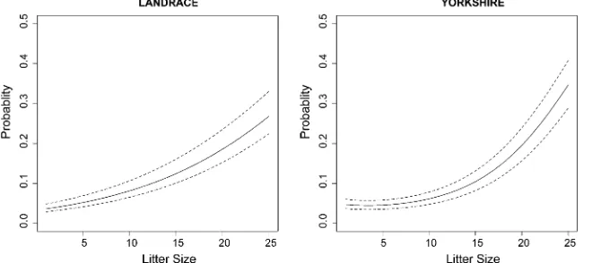
The raw means for litter size for parities 1, 2, 3, and.4 are as follows: 13.4, 15.3, 16.1, and 16.3 for Landrace and 12.3, 14.1, 14.5, and 14.6 for Yorkshire. The average observed proportion of dead-born piglets in parities 1, 2, 3, and .4 are 0.17, 0.17, 0.20, and 0.23 in Landrace and 0.11, 0.09, 0.12, and 0.17 in Yorkshire. Figure 1 shows the raw mortality proportions for a given litter size, across the range of values of

litter size of the data sets, in Landrace and Yorkshire. The

figures provide a rough illustration for the phenotypic rela-tionship between mortality and litter size, especially within the range defined by litter sizes between 7 and 20 in Land-race and between 6 and 19 in Yorkshire. Within this range each point is represented with a minimum of 100 observa-tions, and outside this range, especially at litter sizes,3 and .23 in Landrace, and 4 and 21 in Yorkshire, with,20 obser-vations. The figures indicate that the proportions increase nonlinearly with the size of the litters, but the relationships are a little different in the two breeds (this is more clearly visualized in Figure 4, which displays the probability of mor-tality as a function of litter size, based on the best-fitting models—Model 1 for Landrace and Model 3 for Yorkshire).

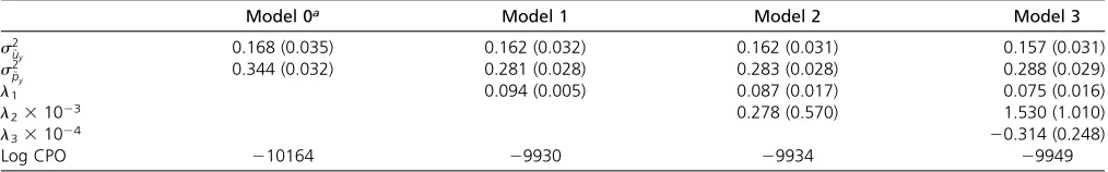
The Monte Carlo estimates of Log CPO (best model has the largest value) indicate that in both breeds, the poorest fit is obtained with Model 0, which assumes that the probability of mortality does not depend on litter size. The differences in the quality of fit are not very marked among the remaining models. For Landrace, the results in Table 1 indicate that a lin-ear relationship (Model 1) gives the best overall fit. The re-gression parameters differ in Yorkshire (Table 2) and the Log CPO indicates that for this breed a cubic relationship (Model 3) between the logit of mortality and litter size gives the best overallfit.

Shown in Table 1 are Monte Carlo estimates of posterior means and posterior standard deviations of various parame-ters in Landrace. In the case of mortality, the ﬁgures in the table indicate that37% of the total variance of the logit of mortality (total variance is equal to s2

~ uyþs

2

py ¼0:443) is accounted for by the residual additive genetic variance (for the best-ﬁtting model, Model 1 for Landrace). These results imply that at the level of the logit for mortality, the additive genetic correlation between mortality and litter size based on Model 1 is0.20 in both breeds [calculated from (9), using estimates of posterior means of the additive genetic variance for litter size,s^2ut 0:8, retrieves an estimate of the genetic correlation l1ð^sut=s^uyÞ 0:09ð0:80=0:16Þ

0:5_¼

0:20]. Simi-lar calculations show that the estimate of the correlation between permanent environmental effects is 0.13 in both breeds. Nielsenet al.(2013) report estimates of the genetic correlation between mortality and litter size ranging between 0.22 and 0.28. However, their analysis treats mortality as a Gaussian trait and the ﬁgures are not directly comparable with the results reported here.

Table 1 Posterior means and standard deviations (in brackets) of variance components, recursive parameters and of LogCPO in Landrace, for mortality

Model 0a Model 1 Model 2 Model 3

s2

~

uy 0.168 (0.035) 0.162 (0.032) 0.162 (0.031) 0.157 (0.031)

s2

~

py 0.344 (0.032) 0.281 (0.028) 0.283 (0.028) 0.288 (0.029)

l1 0.094 (0.005) 0.087 (0.017) 0.075 (0.016)

l231023 0.278 (0.570) 1.530 (1.010)

l331024 20.314 (0.248)

Log CPO 210164 29930 29934 29949

a_{For Model 0,}_s2 ~

uy¼s

2

uy ands

2 ~

py¼s

2

(5)

For Yorkshire (see Table 2), estimates of variances for mortality are broadly similar although the additive genetic variance comprises a somewhat smaller proportion of the total variance of the logit of mortality (26% for Model 3, the best-ﬁtting model in Yorkshire).

The estimates of heritability for litter size in both breeds are very similar. The posterior mean is equal to 0.077 with a posterior standard deviation of 0.020. These estimates are similar to those reported by Suet al.(2007).

We have also studied how predictions of residual additive genetic values for mortality (based on posterior means) differ among the four models. In both breeds, the three product moment correlations between the predictions based on Model 0 and those based on each of the other three models are in the vicinity of 0.96. The three product moment correlations between predictions derived from Models 1, 2, and 3 are all .0.99.

Discussion

In previous work we performed genetic analyses of count data using a number of discrete models (Varona and Sorensen 2010) with an illustration using mortality in pigs. Mortality data show overdispersion, due to a high propor-tion of litter records with an absence of mortality and het-erogeneity induced by covariation among observations. The models accounted for both sources of overdispersion and the study confirmed the presence of genetic variation for mor-tality. The model that showed the best globalfit was a hier-archical binomial logit model and was therefore chosen in this work. In contrast with the models implemented by Varona and Sorensen (2010), in this work the logit of the probability of mortality is assumed to be functionally related to litter size. Both linear and nonlinear functions at the level of the logit were studied and the results indicate that in Landrace, the linear relationship leads to the best global fit. In Yorkshire, quadratic and cubic relationships produce better globalfits and all the models translate into nonlinear relation-ships between the probability of mortality and litter size.

In mixed linear models the interpretation of variance components is straightforward because the random effects operate on the same scale as the values of the response variable. This is not the case in generalized mixed models. One way of studying the direct impact of the variances on the probability of mortality is as follows. Considerﬁrst the

simpliﬁed version (excluding“random effects”) of the model deﬁned in (2), withg1(ti) =l1ti,

ln

fi

12fi

¼miþlti;

wheremiis the mean of theith record (that includes the sum

of the effects herd-year and parity) and ti is the effect of

litter size. For example, in Landrace, replacing the values of the parameters for parity 1 and herd-year 1 by their pos-terior means (resulting in a value ofmi22.5), and using

the posterior mean of l(0.094), translates into a value of the probability

^ fi¼

expm^iþl^ti

1þexpm^_iþ^lti

equal to 0.17 forti= 10 and 0.21 forti= 17. The extended

“mixed model”version of the logit for theith record is

ln

fi

12fi

¼miþltiþqi;

where the random effect qiNð0;s2qÞ is the sum of the

residual additive genetic effect and of the residual perma-nent environmental effect, with s2

q¼s2~uyþs 2

~

p_y. Given mi

andtithe probability fiis a function ofqi, fi¼fðqiÞ ¼

expðmiþltiþqiÞ

1þexpðm_iþltiþqiÞ:

The inverse function is f21_ð_f

iÞ ¼ln½fi=ð12fiÞ2miþlti

and the Jacobian is equal to (fi(12fi))21. Therefore the

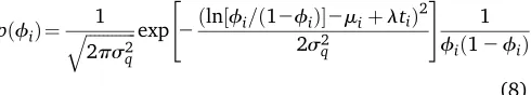
probability density of fiis

pðfiÞ¼

1 ffiffiffiffiffiffiffiffiffiffiffiffi 2ps2 q

q exp

"

2ðln½fi=ð12fiÞ2miþltiÞ2

2s2 q

# 1

fið12fiÞ:

(8) The effect of the variance component on the probability of mortality can be studied using the density (8).

Figure 2 displays the distribution offiforti= 10, where s2

q is replaced by its posterior means^ 2

q¼0:443 (computed

as 0.162 + 0.281; see Table 1). The variance parameters^2q

deﬁnes the range and shape of the distribution in a manner

Table 2 Posterior means and standard deviations (in brackets) of variance components, recursive parameters and of Log CPO in Yorkshire, for mortality

Model 0a Model 1 Model 2 Model 3

s2

uy 0.170 (0.044) 0.165 (0.046) 0.163 (0.045) 0.168 (0.053)

s2

py 0.585 (0.051) 0.494 (0.049) 0.484 (0.049) 0.487 (0.053)

l1 0.121 (0.007) 20.0094 (0.0362) 20.191 (0.046)

l231022 0.473 (0.129) 1.943 (0.306)

l331023 20.371 (0.076)

Log CPO 26363 26185 26181 26176

a_{For Model 0,}_s2 ~

uy¼s

2

uy ands

2 ~

py¼s

2

(6)

that depends on the value ofmi+lti. For example, forti=

10, the 0.1, 0.5, and the 0.9 quantiles arefi= 0.082, 0.173,

and 0.330, respectively, with a mode at fi= 0.131. Ass2q

tends to zero, the distribution offibecomes a point mass at a

value offigiven by the solution to lnðfi=½12fiÞ ¼miþlti

(resulting infi0:17). Theﬁgure shows also the

distribu-tion of the probability of mortality evaluated at the posterior mean of the residual additive genetic variance for mortality ^

s2

~

uy ¼0:162 (dashed lines).

The model speciﬁed by Equations 1 and 2 leads to a simple strategy to reduce mortality, without affecting litter size. Given the model, the residual additive genetic values of mortality are independent of the additive genetic values of litter size. The model predicts, therefore, that selecting on the basis of residual additive genetic values for mortality should not lead to correlated changes in litter size. This lack of association is supported by Figure 3, which discloses the pos-terior distribution of the product moment correlation be-tween the residual additive genetic values of mortality and the additive genetic values of litter size. The value of zero is in a region of very high-density mass.

To give an idea of the likely response to selection to reduce mortality that is expected under the model, we plotted in Figure 4 the range and mean of values of the probability of mortality based on the top and bottom 20% of the distribu-tion of the posterior means of the residual additive genetic values of mortality, for a given value of litter size. The range is

governed by the selection pressure and the variability of the posterior means among individuals. For example, Figure 4 indicates that in the Yorkshire population, for a value of litter size of 14 piglets, the average probability of mortality is 9.14%, and selecting for reduced mortality from the lowest 20% of the distribution changes this probability to 8.16% [a relative change in the proportion of mortality equal to (9.14%28.16%)/9.14%11%]. At a value of litter size of 17, the average probability of mortality is13.24% and select-ing from the lowest 20% changes the probability to 11.88% [a relative change in the proportion of mortality equal to (13.24%211.88%)/13.24%10%]. It is of course possible to retrieve from the MCMC output draws from the marginal distribution of the additive genetic values for mortality uyi using Equation 10 and base selection on these instead.

The classical analysis involving two or more traits is based on a description of their correlation structure at the level of additive genetic and environmental correlations. In this work a recursive parameterization as in Varona et al.(2007) was chosen instead. In this parameterization, a one-way causal path establishes a direct effect of the size of the litter on mortality, omitting the details of the underlying nature of this relationship. A graphical representation of this relationship is in Figure 4. The models that condition the logit of mortality on litter size retrieve estimates of residual (additive genetic and permanent environmental) variances, in contrast to Model 0, which provides estimates of marginal variances. Theﬁgures in Table 1 and Table 2 illustrate this, especially for the total variance of the logit of mortality (given by

s2

~ uyþs

2

~

p_y). Although the signal is not strong for each of the

terms taken separately, their sum is clearly larger for Model 0 (which yields instead estimates ofs2

uyþs 2

py) than for the remaining models, in both breeds.

From a practical point of view it is relevant to compare the predictive ability of this model with the one currently in operation in the Danish pig-breeding program. In the latter, the traits analyzed are total number born and total number born alive, from which parameters associated with number of piglets dead are derived. The model is based on multivariate normality and ignores the truncated nature of one of the traits (number born alive is smaller or equal to total number born). However, it has the appeal of ease of implementation,

Figure 2 Probability distribution of the probability of mortality forti= 10.

Solid line,s2

q¼0:443; dashed lines2~uy¼0:162.

Figure 3Monte Carlo posterior distribution (in

(7)

from the point of view of both computing requirements and data collection. Details of this model can be found in Suet al. (2007) and Nielsenet al.(2013). The comparison presented here for each breed is based on a 10-fold cross-validation (for example, Hastie et al. 2009), whereby the total number of sows with records were divided into 10 groups of equal size. Phenotypic records of each fold were excluded in the training phase, predicted in the validating data set, and the correla-tion between observed and predicted number of dead piglets in the validating data set was computed. The predictions of the number of dead piglets using both models are obtained conditional on observed total number of piglets born. We label the model currently in operation by MVN (multivariate normal), and the binomial-normal model by BN. The average correlations (over the 10 folds) in Landrace based on MVN and on BN are 0.52 and 0.57, respectively. In Yorkshire, the correlations are 0.46 (MVN) and 0.50 (BN). Thefigures in-dicate that the BN model has a small advantage in terms of predictive ability. However, a breeding program involves a large number of traits and further work is needed, including refinements of the model to account for possible effects of the sire on mortality (Strangeet al.2013), to study the feasibility of incorporating the BN model into a system that can yield routine predictions of aggregate genotypes in a computation-ally efficient manner.

We have investigated the properties of the logit model for mortality and the Gaussian model for litter size using a mod-estly sized data set. In this investigation no attempt was made at exploring efﬁcient MCMC algorithms. An implementation on a larger scale requires more attention to algorithmic details, especially if the model is extended to include dense genetic marker information. This should be the subject of future studies.

The Landrace and Yorkshire data and pedigree ﬁles as well as the FORTRAN code used forﬁtting the models can be found in supporting information,File S1.

Acknowledgments

Theﬁnal manuscript beneﬁted from criticism and suggestions from two reviewers and the editor. The work was funded by the Green Development and Demonstration Programme

(grant no. 3405-11-0279) of the Danish Ministry of Food, Agriculture and Fisheries, the Pig Research Center, and Aarhus University.

Literature Cited

Arango, J., I. Misztal, S. Tsuruta, M. Culbertson, J. W. Hollet al., 2006 Genetic study of individual preweaning mortality and birth weight in large white piglets using threshold linear mod-els. Livest. Sci. 101: 208_–218.

Blasco, A., J. P. Bidanel, and C. Haley, 1995 Genetics and neonatal survival, pp. 17_–38 inThe Neonatal Pig: Development and Survival, edited by M. A. Varley. CAB International, Wallingford, UK. Cheverud, J. M., 1984 Quantitative genetics and developmental

con-straints on evolution by selection. J. Theor. Biol. 110: 155–171. de los Campos, G., D. Gianola, P. Boettcher, and P. Moroni,

2006 A structural equation model for describing relationships between somatic cell score and milk yield in dairy goats. J. Anim. Sci. 84: 2934–2941.

Duncan, O. D., 1975 Introduction to Structural Equation Models. Academic Press, San Diego, CA.

Gelfand, A. E., 1996 Model determination using sampling-based methods, pp. 145–161 inMarkov Chain Monte Carlo in Practice, edited by W. R. Gilks, S. Richardson, and D. J. Spiegelhalter. Chapman & Hall, London.

Gianola, D., and D. Sorensen, 2004 Quantitative genetic models describing simultaneous and recursive relatiosnhips between phenotypes. Genetics 167: 1407_–1424.

Goldberger, A. S., 1972 Structural equation methods in the social sciences. Econometrica 40: 979_–1001.

Hastie, T., R. Tibshirani, and J. Friedman, 2009 The Elements of

Statistical Learning. Springer, New York.

Henderson, C. R., 1984 Applications of Linear Models in Animal

Breeding. University of Guelph, Guelph, Ontario, Canada.

Jöreskog, K. G., 1973 A general method for estimating a linear structural equation system, pp. 85–112 inStructural Equation

Models in the Social Sciences, edited by A. S. Goldberger, and

O. D. Duncan. Seminar, New York.

Lande, R., 1979 Quantitative genetic analysis of multivariate evo-lution, applied to brain:body allometry. Evolution 33: 402–416. Nielsen, B., G. Su, M. S. Lund, and P. Madsen, 2013 Selection for increased number of piglets at dayﬁve after farrowing has in-creased litter size and reduced piglet mortality. J. Anim. Sci. 91: 2575_–2582.

Roehe, R., and E. Kalm, 2000 Estimation of genetic and environ-mental risk factors associated with pre-weaning mortality in piglets using generalized linear mixed models. Anim. Sci. 70: 227_–240.

Figure 4 Posterior means of the average

(8)

Sorensen, D., A. Vernersen, and S. Andersen, 2000 Bayesian anal-ysis of response to selection: a case study using litter size in Danish Yorkshire pigs. Genetics 156: 283–295.

Strange, T., B. Ask, and B. Nielsen, 2013 Genetic parameters of the piglet mortality traits stillborn, weak at birth, starvation, crushing, and miscellaneous in crossbred pigs. J. Anim. Sci. 91: 1562–1569.

Su, G., M. S. Lund, and D. Sorensen, 2007 Selection for litter size at dayﬁve to improve litter size at weaning and piglet survival rate. J. Anim. Sci. 85: 1385–1392.

Van Arendonk, J. A. M., C. Van Rosmeulen, L. L. G. Janss, and E. F. Knol, 1996 Estimation of direct and maternal genetic (co)var-iances for survival within litters of piglet. Livest. Prod. Sci. 46: 163_–171.

Varona, L., and D. Sorensen, 2010 A genetic analysis of mortality in pigs. Genetics 184: 277–284.

Varona, L., D. Sorensen, and R. Thompson, 2007 Analysis of litter size and average litter weight in pigs using a recursive model. Genetics 177: 1791–1799.

Walsh, B., 2003 Evolutionary quantitative genetics, pp. 380–442

inHandbook of Statistical Genetics, Vol. 1, edited by D. J.

Bald-ing, M. Bishop, and C. Cannings. John Wiley, Chichester, UK. Wright, S., 1921 Correlation and causation. J. Agric. Res. 210:

557–585.

Xiong, M., J. Li, and X. Fang, 2004 Identi_ﬁcation of genetic net-works. Genetics 166: 1037_–1052.

(9)

Appendix

The model for the joint distribution of additive genetic and permanent environmental values for mortality and litter size

The independence of the residual additive genetic values for mortality and additive genetic values for litter size is based on the following result. A recurrent formulation for the additive genetic values for mortality and litter size for an individual is (Varonaet al.2007)

uyi;uti

N " 0 0

; s2uy ls

2 ut ls2

ut s

2 ut

!#

; (A1)

wherelis a recurrent parameter that describes the linear relationship between mortality and litter size. Then,

uyiuti

Nhluti;s

2 uy2l

2_s2 ut i

:

We can write

uyi¼E

uyiuti

þ~uyi; (A2)

where~uyi is the residual term in the additive genetic regression of mortality on litter size and is referred to as the residual additive genetic value of mortality. Then,

~ uyi;uti

N " 0 0 ; s 2 ~ uy 0 0 s2 ut

!#

; (A3)

where s2

~ uy ¼s

2 uy2l

2_s2

ut. The covariance matrix of the joint distribution of the vectors u~y and ut is G 5 A, whereG¼diagðs2

~ uy;s

2

utÞis the diagonal covariance matrix of (A3). Therefore the joint distribution factors into the product of the marginal distributions; that is,

p~uy;utjA;s2_~uy;s

2 ut

¼p~uyA;s2u_~y

putjA;s2ut

:

In the case of the permanent environmental values, the starting point is

pyi;pti N " 0 0

; s2py ls

2 pt ls2

pt s

2 pt

!#

; (A4)

which in a similar manner leads to

~ pyi;pti

N " 0 0 ; s 2 ~ py 0 0 s2pt

!#

: (A5)

Sketch of the MCMC algorithm

The fully posterior distributions of the parameters, except for the variance components, do not have closed forms. For example, updating thejth element ofayrequires the computation of its fully conditional posterior distribution

p

a

y;j

all

;

y

;

t

}

Q

n

i¼1

h

_exp

_ð

_x

i9ayþzi9~uyþwi9pyþgðtiÞ

Þ

1þexp

ð

x9ayþz9i~uyþwi9pyþgðtiÞ

Þ

i

yiI

ð

xi9ay¼ay;j

Þ

3

1

2

₁_þexp_exp

ð

x

_ð

i9_xayþz9i~uyþw9ipyþgðtiÞ

Þ

i

9_a_y_þzi9u~yþwi9pyþgðtiÞ

Þ

ðti2yiÞI

ð

xi9ay¼ay;j

Þ

;

(A6)

(10)

GENETICS

Supporting Information

http://www.genetics.org/lookup/suppl/doi:10.1534/genetics.113.159475/-/DC1