1
STABILITY ANALYSIS AND SEMI-ANALYTIC SOLUTION TO A SEIR-SEI
MALARIA TRANSMISSION MODEL USING HE’S VARIATIONAL ITERATION
METHOD
1. AKINFE, Timilehin Kingsley* 2. LOYINMI, Adedapo Chris 1, 2Department of Mathematics, Tai Solarin University of Education, Ijagun,
Ijebu ode, Ogun state, Nigeria; [email protected]*; [email protected] 1 ORC-ID: 0000-0002-5308-7053*; 2 ORC-ID: 0000-0002-6171-4256
*Correspondence: [email protected]
Abstract:
We have considered a SEIR-SEI Vector-host mathematical model which captures malaria
transmission dynamics, described and built on 7-dimensional nonlinear ordinary differential
equations. We compute the basic reproduction number of the model; examine the positivity and
boundedness of the model compartments in a region using well established methods viz:
Cauchy’s differential theorem, Birkhoff & Rota’s theorem which verifies and reveals the
well-posedness, and carrying capacity of the model respectively, the existence of the Disease-Free
(DFE) and Endemic (EDE) equilibrium points were determined and examined
Using the Gaussian elimination method and the Routh-hurwitz criterion, we convey stability
analyses at DFE and EDE points which indicates that the DFE (malaria-free) and the EDE
(epidemic outbreak) point occurs when the basic reproduction number is less than unity (one)
and greater than unity (one) respectively.
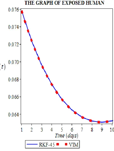
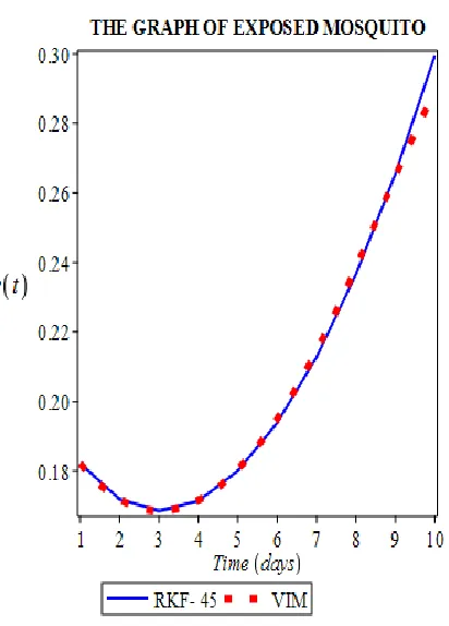
We obtain a solution to the model using the Variational iteration method (VIM) (an
unprecedented method) to each population compartments and verify the efficacy, reliability and
validity of the proposed method by comparing the respective solutions via tables and combined
plots with the computer in-built Runge-kutta-Felhberg of fourth-fifths order (RKF-45).
2
We illustrate the combined plot profiles of each compartment in the model, showing the dynamic
behavior of these compartments; then we speculate that VIM is efficient and capable to conduct
analysis on Malaria models and other epidemiological models.
Keywords:
SEIR-SEI, Basic Reproduction number, Disease-Free equilibrium point (DFE), Endemic
equilibrium point, Stability, Variational iteration method (VIM), Runge-Kutta-Felhberg
(RKF-45).
1. Introduction
Malaria is a mosquito-borne infectious disease that is life threatening to humans and other
animals (Malaria fact sheet, 2014) [16]. This infectious disease is widely spread throughout the
globe and predominantly present in tropical and sub-tropical regions of the earth including some
parts of Europe.
The wide spread of this vector-borne disease (malaria) has urged numerous researchers and
health organizations to study the epidemiology and transmission dynamics of the disease; so as
to be able to implement an appropriate intervention strategy on its ubiquitous nature.
Because of its nature of being a fatal disease, this is why 25th of April is set aside as the world’s annual malaria day for the global alertness against the disease. Malaria causes symptoms that
typically include fever, tiredness, vomiting, and headaches (Caraballo, 2014). In severe cases it
can cause yellow skin, seizures, coma, or death. (Caraballo, 2014) [15]. These symptoms usually
begin ten to fifteen days after being bitten by an infected mosquito and if not properly treated,
people may have recurrences of the disease months later (Malaria fact sheet W.H.O, 2014) [16].
Malaria is caused by single-celled microorganisms of the plasmodium group (Malaria Fact sheet
W.H.O, 2014). The disease is most commonly spread by an infected female Anopheles
mosquito. The mosquito bite introduces the parasites from the mosquito’s saliva into the Host
(Human). There are five different plasmodium species leading to malaria infection and disease
among humans; These are: Plasmodium Falciparum (P. falciparum), Plasmodium vivax (P.
vivax), Plasmodium Ovale (P. ovale), Plasmodium malariae (P. malariae), Plasmodium
3
Most deaths are caused by P. falciparum as it is the most dangerous of all plamodium species [8,
13]. P. vivax, P. ovale, and P. malariae generally cause milder form of malaria while the P.
knowlesi rarely cause disease in humans. This P. falciparum is mainly found in Africa as it is
common and causing deaths worldwide. In addition, Plasmodium knowlesi is a type of malaria
that infects macaques in Southeast Asia; also infect humans causing malaria that is transmitted
from animal to human (zoonotic malaria) [8, 13-14].
WHO Malaria report (2013) shows that approximately 80% of malaria cases and 90% of deaths
are estimated to occur in most countries of this sub-Saharan Africa [9]. In 2015, WHO estimates
that 212 million clinical cases of malaria occurred and 429,000 people died of malaria, most of
them were children in Africa [10]. The world Malaria Report in 2018 [38] shows an
unprecedented period of success in global malaria control. An estimated 219 million cases of
malaria occurred worldwide (95% confidence interval (CI): 203-262 million), compared with
239 million cases in 2010 (95% CI: 219-285 million) [11] and 217 million cases in 2016 (95%
CI: 200-259 million) [12] with 92% cases in the African region, 5% in the South-East Asia
region and 2% in the WHO Eastern Mediterranean region.
Very recently, in the common wealth malaria reports (April, 2019) [39]; a historic partnership of
governments, civil society, the private sector and multilateral organizations, came together in
London for a momentous malaria summit. Delivering US $4.1 billion for the global malaria fight
and two days later at the commonwealth heads of Government meeting (CHOGM), all 53 leaders
committed to halve malaria in the commonwealth within five years.
The report here shows that the commonwealth countries: The Gambia, Belize, Bangladesh, India,
Malaysia, Mozambique and Nigeria are already on a trajectory to achieve the target to halve
malaria in 2023. See [39].
Due to the everyday attempt to control the epidemic and prevalent nature of malaria, several
models have been developed by mathematicians; so as to understand the transmission dynamics
of this infectious disease and implement a control strategy. Majority of these models are being
described by differential equations of the nonlinear type. The first malaria model for malaria
4
(1957) [5] considering some biological assumptions. Since then, many models have been
developed like Ngwa and Shu (1999) [18] Jia Li (2011) [3], Prashant Goswami et al (2012) [20],
Olaniyi S and Obabiyi (2013) [2], Shah NH and Gupta. J (2013) [21], Hal-Feng Huo and
Guang-ming Qiu(2014) [23], Altaf Khan et al (2015) [22], Oti eno (2016), Osman et al (2017) [1],
Osman et al (2018) [24], Traore Bakare (2018) [7] to mention a few. Researchers and
mathematicians have endeavored to proffer solution to these models including that of malaria via
different methods so as to understand the transmission dynamics better in Nigar Ali et al. (2019)
using Adomian Decomposition method [25], Abioye adesoye idowu et al (2018) using
Differential transform method [28], Peter olumuyiwa james et al (2018) solved using Multi-step
Homotopy analysis method [30]. Morufu oyedunsi olayiwola (2017) using the Variational
iteration method solved a SEIRS epidemic model [26]. Yullita molliq Rangkuti (2014) obtained
a numerical analytical solution of SIR model of Dengue fever disease in South sulawesi using
HPM and VIM [19], Fazal Haq et al (2017) by Laplace Adomian decomposition method solved
an epidemic model of a vector borne disease [17].
Of all the semi-analytical methods implemented to solve epidemic models including malaria,
none have solved the malaria model using the variational iteration method and as a result, less
attention has been paid using this method on malaria models. This method is unprecedented.
The main reason of this paper is to validate the efficiency of variational iteration method and also
speculate its capability as alternative approach in solving and analyzing epidemiological models
including malaria.
The huge advantage of this method over other methods include: the simplicity and
straight-forwardness, less computational stress or efforts of the method with no linearization of the
nonlinear term, no computation of Adomian or He’s polynomials, yet yielding highly accurate
and rapidly convergent results devoid of errors when compared numerically and graphically.
In this research, we consider an existing SEIR model of Osman et al (2017), conduct a stability
analysis, and then obtain semi-analytic solution via Variational iteration method (VIM).
The model presented here in this research is of two compartmental system of nonlinear ordinary
differential equation involving the host which is the human and the Vector which is the
mosquito. The human (host) is described by four differential equations and the mosquito by three
5
The subsequent organization of this research work is structured as follows: Section 2 elucidates
the compartmental model of the malaria transmission dynamics as well as the flow diagram of
the model; Section 3 focuses on the mathematical analysis of the model which includes the
analysis on the feasible region of the model, so as to verify the epidemiological validity of the model; the disease-free equilibrium point (DFE), basic reproduction number, the endemic
equilibrium point (EDE), stability of the DFE via Gaussian elimination method and the EDE
with theorems, lemmas, and proofs were all computed here.
Semi-analytic solution was then proffered to the seven (7) compartments of the vector-host
model using He’s variational iteration method (VIM) in Section 4.
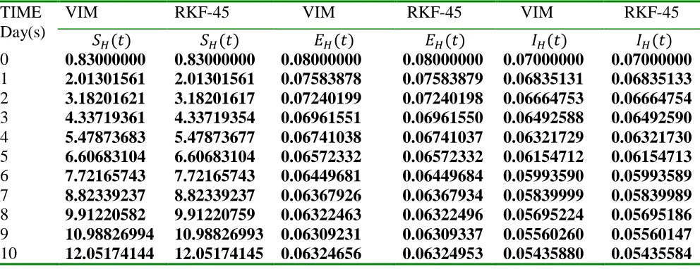
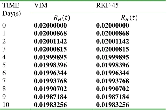
Lastly, numerical result comparison were made for the solved compartments via tables and
combined plots of Runge-Kutta-Felhberg 45 (RKF-45) and VIM, results were then interpreted
and discussed before the final conclusion in section 5 and 6 respectively.
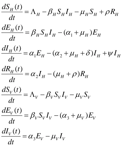
2. The Model
The model consists of two classes of population, the human population and the mosquito
population. The human 𝑁 population is subdivided into four compartments, the susceptible, the exposed, the infected, and the recovered. While the mosquito 𝑁 population is subdivided into three compartments, the susceptible, the exposed, the infected as it is assumed that mosquitoes
don’t recover. We then have that the 𝑆𝐸𝐼𝑅 model for the humans (host) and the 𝑆𝐸𝐼 model for
the mosquito (vector). (Table 1)
2.1 Model Assumptions
The Population of the susceptible human
S
H(
t
)
is increased by the recruitment of individuals at a rateH, and by the recovered individuals returning back to the compartment due to loss of immunity at a rate 𝜌, they acquire infection at a rate 𝛽𝐻, the population is thendecreased by natural death of humans at a rate 𝜇𝐻. (Fig 1) The population of the Exposed human
)
(
t
6
humans whose infection has developed to the infectious compartment at a rate 𝛼1 , and further decreased by natural death 𝜇𝐻. (Fig 2)
The population of the infected
I
H(
t
)
is generated by humans who are infectious at a rate 𝛼1,increased by newborn baby with infection at rate 𝜓 , then decreased by natural death 𝜇𝐻 ,
malaria induced death, and humans who have recovered at rates 𝜇𝐻 , 𝛿 , and 𝛼2 respectively. (Fig 3)
The Recovered population
R
H(
t
)
is generated by those who are infected but are being treated and recovering from malaria at a rate 𝛼2. It is then decreased by those who die naturally and losetheir immunity at rates 𝜇𝐻 and 𝜌 respectively. (Fig 4)
The susceptible mosquito population
S
V(
t
)
is generated by the recruitment of mosquitoes intothe compartment at a rateᴧ𝑉, decreased by infection and death by natural cause with rates 𝛽𝑉
and 𝜇𝑉. (Fig 5)
The Exposed mosquito’s population
E
V(
t
)
is generated by susceptible mosquitoes exposed tothe malaria pathogen infection at a rate 𝛽𝑉, decreased by mosquitoes that have developed into the infectious state, and by natural cause at rates 𝛼3 , and 𝜇𝑉. (Fig 6)
The Infected mosquito’s population IV(t) is generated by exposed mosquito whose state has moved to the infectious state at the rate 𝛼3, and decreased by natural cause 𝜇𝑉. (Fig 7)
𝝁𝑯
𝜓
𝜌
𝑺𝑯(𝒕) 𝑬𝑯(𝒕) 𝑰𝑯(𝒕) 𝑹𝑯(𝒕)
𝝁𝑯
𝝁𝑯 𝜹 𝝁𝑯
𝜷𝑯𝑺𝑯𝑰𝑯
ᴧ
𝑯𝜶𝟏 𝜶𝟐
𝑺𝑽(𝒕) 𝑬𝑽(𝒕) 𝑰𝑽(𝒕)
𝝁𝑽 𝝁𝑽
𝜷𝑽𝑺𝑽𝑰𝑽
𝝁𝑽
ᴧ
𝑽7
1
1 2
2
3
3
( )
( )
( )
( )
( )
( )
( )
( )
( )
( )
( ) H
H H H H H H H
H
H H H H H
H
H H H H
H
H H H
V
V V V V V V
V
V V V V V
V
V V V
dS t
S I S R
dt dE t
S I E
dt dI t
E I I
dt dR t
I R
dt dS t
S I S
dt dE t
S I E
dt dI t
E I
dt
(1)
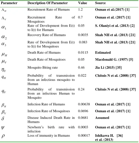
Table 1: State Variables and parameter description of the SEIR-SEI model
State Variables Description
𝑺𝑯(𝒕) Susceptible Human at time t
𝑬𝑯(𝒕) Exposed Human at time t
𝑰𝑯(𝒕) Infected Human at time t
𝑹𝑯(𝒕) Recovered Human at time t
𝑺𝑽(𝒕) Susceptible mosquito at time t 𝑬𝑽(𝒕) Exposed mosquito at time t
𝑰𝑽(𝒕) Infected mosquito at time t
Parameters Description
ᴧ𝑯 Recruitment rate of Humans
8
𝜶𝟏 Development from exposure to being infectious (Humans)
𝜶𝟐 Recovery rate of Humans
𝜶𝟑 Development from exposure to being infectious (mosquito)
𝝁𝑯 Natural Death of Humans
𝝁𝑽 Natural Death of Mosquitoes
𝜹 Malaria induced death rate for Humans
𝒒𝑯 Probability of transmission from an infectious mosquito to a susceptible
Human
𝒒𝑽 Probability of Transmission from an infectious Human to a susceptible mosquito
𝜼𝑽 Mosquito Biting Rate
𝜷𝑯 Infection rate of Humans( 𝑞𝐻 × 𝜂𝑉)
𝜷𝑽 Infection rate of Mosquito (𝑞𝑉× 𝜂𝑉)
𝝆 Loss of Immunity for Humans
𝝍 Newborn’s birth with infection
3.0 MATHEMATICAL ANALYSIS OF THE MODEL
3.1 Positivity and Boundedness of Solution
Here, results are presented and verifications are made as to guarantee that the malaria model
governed by the system (1) is epidemiologically and mathematically well-posed in a feasible
region; given by: 4 3
9 Where, . 0 , 0 , 0 , : ) , , ( , 0 , 0 , 0 , 0 , : ) , , , ( 3 4 V V V V V V V V V V V V H H H H H H H H H H H H H H H I E S I E S I E S R I E S R I E S R I E S
3.1.1 Theorem 1:
The feasible region of the system (1) given by
0 , 0 , 0 , 0 , 0 , 0 , 0 ; ) ( ) ( ) ( ; ) ( ) ( ) ( ) ( : ) , , , , , , ( V V V H H H H V V V V V H H H H H H V V V H H H H I E S R I E S t I t E t S t R t I t E t S I E S R I E S
is a positive invariant set and Bounded.
Proof: Let us consider the Host Population governed by the system
H H H H H H H H H H H H H H H H H H H H H H H R I dt t dR I I E dt t dI E I S dt t dE R S I S dt t dS ) ( ) ( ) ( ) ( ) ( ) ( ) ( 2 2 1 1
(2)
) ( ) ( ) ( )(t E t I t R t
S
NH H H H H is the human net population. Now from the derivatives of sums;
( ) ( ) ( ) ( ) ( )
H H H H H
dN t dS t dE t dI t dR t
dt dt dt dt dt
(3)
This implies that,
1
1 2 2
( )
(
) (
(
)
)
(
(
)
) (
(
)
)
H
H H H H H H H H H H H H
H H H H H H H
dN
t
S I
S
R
S I
E
dt
E
I
I
I
R
10
This implies that H H HNH dt
t
dN ()
when we remove the parameter( )IH.
( )
H
H H H
dN t
N
dt
(4)
By solving the first order linear differential inequality (4) using integrating factor method we
have;
( ) H Ht
H
H
N t pe
(5)
Where pis a constant of integration.
Then by applying Birkhoff and Rota’s theorem [31] on the differential inequality (5), it follows
that
lim
( )
HH t
H
N
t
(6)
This is commonly known as the carrying capacity of the system and hence shows Boundedness.
It then follows that
H H H
H H
H
H t S t E t I t R t
N
4 ) ( ) ( ) ( ) ( )
(
This proves the boundedness of the solution inside the region H
Now for other classes of the population we have;
3.1.2 Other Compartments
We consider the rate of change of the population in the Susceptible Human compartment
( )
H
H H H H H H H
dS t
S I S R
dt (7)
H H H
H H HH I S R
dt t
dS
( )
Let
H
HIH
H,Then, H H H H
H
S
R
dt
t
dS
(
)
11
( )
0
H
H H
dS t
S
dt
(9)
By separation of variables we obtain that;
( ) H
H H
dS t
dt S
(10)
c t H
H H
e e
t S
c t t
S
H
) (
) ( ln
Let
A
e
cthen we have;S
H(
t
)
Ae
Ht
At the initial state when
t
0
, SH(0)A0.0
)
0
(
)
(
t tH H
H
H
Ae
e
S
t
S
Holds and this implies thatS
H(
t
)
0
holds.Indicating that
S
H(
t
)
stays and remains positive.Similarly, we consider the non-linear ODE for the exposed human
1
( )
( )
H
H H H H H
dE t
S I E
dt
1 ( )
( )
H
H H H H H
dE t
E S I
dt
(11)
From
HS
HI
Hon the right hand side of the equation (11), we have thatS
H
0
,
S
H
0
fromour previous proof. Now forIH 0we have that H( )( 1 H)EH 0
dt t
dE
when IH 0 and
0 )
( ) (
1
H H
H E
dt t
dE
when
I
H
0
;1
( )
(
)
0
H
H H
dE
t
E
dt
(12)
Solving the differential inequality (12) using separation of variable
We have
1
( )
( )
H
H H
dE t
dt E
12
Let
H
(
1
H)
( ) H
H H
dE t
dt
E
ln
( ) H
H H
t c H
E t c
E t e e
When
t
0
, we have0
)
0
(
)
(
0
)
0
(
)
0
(
0
t H
H H H
H
e
E
t
E
A
E
A
Ae
E
Hence,
E
H(
t
)
0
Holds.Similarly, we consider the nonlinear differential equations of other state variables 𝐼𝐻(𝑡) and 𝑅𝐻(𝑡) of the Infected and the recovered class; we let H (2H )and H (H ) respectively and solve the differential inequalities 𝑑𝐼𝐻
𝑑𝑡 + 𝛾𝐻𝐼𝐻 ≥ 0, 𝑑𝑅𝐻
𝑑𝑡 + 𝜀𝐻𝑅𝐻 ≥ 0 with the
initial conditions.
We obtain the solutions to the ODEs and we have that
I
H(
t
)
0
andR
H(
t
)
0
holdrespectively.
3.1.3 Mosquito Model (Vector)
We consider the governing equation of the vector (SEI) model which is the Mosquito.
V V V V
V V V
V V V
V V V V V V V
I E dt
t dI
E I
S dt
t dE
S I S dt
t dS
3
3
) (
) (
) (
) (
(14)
The total Population density gives
( ) ( ) ( ) ( )
V V V V
13
( ) ( ) ( ) ( )
V V V V V V V
V V V
dN t N t dS N t dE N t dI
dt S dt E dt I dt
(16)
We have that
( ) ( ) ( )
1,
V V V
V V V
N t N t N t
S E I
(17)
( )
V V V V
dN t dS dE dI
dt dt dt dt
3
3
( )
( )
V
V V V V V V V V V V V V V V
dN t
S I S S I E E I
dt
(18)
We then have,
( )
V
V V V
dN t
N
dt
(19)
By solving the differential inequality by method of integrating factor and apply Birkhoff and
Rota’s theorem [31]
V V V
t N t
( )
lim (20)
It then follows that
V V V
V V
V t S t E t I t
N
( ) ( ) ( ) )
(
This proves boundedness.
Similarly as the Host model, 𝑆𝑉(𝑡) > 0, 𝐸𝑉(𝑡) ≥ 0, 𝐼𝑉(𝑡) ≥ 0 holds for the mosquito population.
This completely proves our theorem 1.
3.2 Disease-Free equilibrium points and the Reproduction Number
The points at which the differential equation is equal to zero are referred to as the equilibrium
points or steady-state solutions.
The model consists of just two equilibrium points which is the disease-free and the Endemic
equilibrium points
The point or time at which the disease wiped out and the entire population is susceptible is the
Disease-free equilibrium point while the point at which the disease persists in the population
14
At Equilibrium,
( )
( )
( )
( )
( )
( )
( )
0
V V V
H H H H
dS t
dE t
dI t
dS
t
dE
t
dI
t
dR t
dt
dt
dt
dt
dt
dt
dt
(21)By substituting (21) into the system of equations (1),
0 0 3 0 3 0 0 0 0 0 0 0 2 0 0 2 0 1 0 1 0 0 0 0 0 0 0 ) ( 0 0 ) ( 0 ) ( 0 ) ( 0 0 V V V V V V V V V V V V V V H H H H H H H H H H H H H H H H H H H I E E I S S I S R I I I E E I S R S I S
Then the DFE for the SEIR-SEI system is given by:
0 0 0 0 0 0 0 0
, , , , , , H , 0, 0, 0, V , 0, 0, 0
H H H H V V V
H V
E S E I R S E I
(22)
3.2.1 The Basic Reproduction Number R0 of the SEIR-SEI Model of Malaria Transmission
An important concept of Epidemiological models is the basic reproduction number which is
usually denoted byR0,this number is the average number of secondary infections in the EH(t)
compartment, infected by an infectious individual in the IH(t) compartment in a completely susceptible population. The Reproduction number in this model would be calculated using the
Next generation matrix method. Since our model is a vector-Host model, we define the Next
generation as a square matrix ‘G’ in which the individual of type j which accounts for the
infection using the reproduction number assuming that the population of type i is susceptible
[21, 6].
The assumption that the population is susceptible implies that the reproduction number would be
computed at DFE point. Since there are two classes of population, we have the 2×2 matrix
0 11 12 0 21 22 0 0 V H R g g G R g g
15
Let the reproduction number of the model be denoted by 𝑅𝐺.
From |GI| 0
where is an identity matrix.
|GI |2R0HR0V 0
(24)
0H 0V
R R
0 0
G H V
R R R
(25)
From the human nonlinear system of ODEs;
H H H H
H H H H
H
H H H
H H H
H H H H H H H H
R I
dt t dR
I I E
dt t dI
E I
S dt
t dE
R S I S dt
t dS
) ( )
(
) (
) (
) ( )
( ) (
2 2 1
1
Using the next generation matrix method,
Let
TH H H
H I S R
E
X , , , (26)
Then
1
1 2
'
2
( )
( )
( )
H
H H H H H
H
H H H H
H H
H H H H H H H
H
H H H
H dE
dt
S I E
dI
E I I
dX dt
X
S I S R
dS dt
dt I R
dR dt
(27)
16 1 1 2 2 ( ) ( ) 0 0 ( ) 0 H H
H H H
H H H H
H
H H H H H H H
H H H
E S I
E I I
dX
S I S R
dt I R (28)
This is now in the form
( ) ( )
H
i i
dX
F X V X
dt (29)
1 1 1
2 1 2 2
3 3
4 2 4
( ) ( ) 0 ( ) ; ( ) 0 ( ) 0 H H
H H H
H H H H
i i
H H H H H H H
H H H
F E V
S I
F E I I V
F X V X
F S I S R V
F I R V
Where F Xi( ) is the matrix of new infections and V Xi( )is the matrix of other transfer terms [6]
The next step here is to linearize the matrix F Xi( ) andV Xi( )by taking the jacobian of each term in the matrices at Disease free equilibrium point .
Let J F X
i( )
FHand J V X
i( )
VH( ) ( )
,
i i
H H
j j
F X V X
F V
X X
At DFE
0 0
0 ( ) 0 ( )
( ) i , ( ) i
H H
j j
F E V E
F E V E
X X
0 0 0 0
1 1 1 1
0 0 0 0
2 2 2 2
0
0 0 0 0
3 3 3 3
0 0 0 0
4 4 4 4
( ) ( ) ( ) ( ) ( ) ( ) ( ) ( ) ( ) ; ( ) ( ) ( ) ( ) ( ) ( ) ( ) ( )
H H H H
H H H H
i j
H H H H
H H H H
F E F E F E F E
E I S R
F E F E F E F E
E I S R
F E V
X F E F E F E F E
E I S R
F E F E F E F E
E I S R
0 0 0 0
1 1 1 1
0 0 0 0
2 2 2 2
0
0 0 0 0
3 3 3 3
0 0 0 0
4 4 4 4
( ) ( ) ( ) ( )
( ) ( ) ( ) ( ) ( )
( ) ( ) ( ) ( )
( ) ( ) ( ) ( )
H H H H
H H H H
i j
H H H H
H H H H
V E V E V E V E
E I S R
V E V E V E V E
E I S R
E
X V E V E V E V E
E I S R
V E V E V E V E
E I S R
For the Reproduction number, we only need terms in the Exposed and the infected compartments
[27].
17
1 1 2 0 0 ; 0 0 H H H H H H HF
V
HR
0 Is the spectral radius or dominant Eigen value of
1
H H
V
F
that is
FHVH1
I 0; I is an identity matrix.By computing the spectral radius, the reproduction number is given as;
1 0 1 2 ( )( ) H H H
H H H
R
(30)Similarly, by considering the nonlinear system in the Mosquito’s model
V V V V V V V V V V V V V V V V V I E dt t dI E I S dt t dE S I S dt t dS 3 3 ) ( ) ( ) ( ) (
Similarly, using the Next generation matrix approach on the vectors system of equations above
we have the Mosquito’s reproduction number as
3 0 3
(
)
V V V V VR
(31)From equation (25) we have that
R
G
R
0HR
0V then by putting the equation (30) and (31) into(25) we have the general reproduction number of the SEIR-SEI system as:
)
)(
)(
(
1 3 22 3 1
H V H V H V H V H GR
(32)This gives the reproduction number of the complete system
By alternative notations, if we let
1 3 2
(
)
(
)
(
)
H H V V H H
(33)18
Then,
1 3 2
H V H V G
H V H V H
R
(33)2 1 3 2
H V H V G
H V H V H
R
(34)
3.3 Existence of the Endemic Equilibrium Points
The SEI-SEI model of Malaria transmission possesses an endemic equilibrium point
* * * * * * * *
, E , I , R , , E , I
H H H H V V V
E S S (35)
At this point, there is persistence of the disease in the system and hence an epidemic outbreak.
At equilibrium,
0
)
(
)
(
)
(
)
(
)
(
)
(
)
(
dt
t
dI
dt
t
dE
dt
t
dS
dt
t
dR
dt
t
dI
dt
t
dE
dt
t
dS
H H H H V V VThen,
0 0 0 0 0 0 0 * * 3 * 1 * * * * * * * 1 * 2 * 1 * 1 * * * * * * V V V V V V V V V V V V V V H H H H H H H H H H H H H H H H H H I E E I S S I S R I I E E I S R S I S (36)We solve the system of equation (36) simultaneously for the corresponding endemic point
s. From 01EH* (2H )IH* IH* in the system, we can write that
* *
1EH ( 2 H )IH
Thus we have
*
* 2
1
( H ) H
H
I
E
19
Put (37) into dSH(t)
dt we have the relation,
1
2
1
0
H H H
H H H
I
S I
(38)
This implies that
1
2
1
0
H H
H H H
I S
Where
I
H
0
1
2
1
0
H H
HSH
;
1
2
*
1
H H
H
H
S
(39)
Again fromdRH(t)
dt , we have
* * 2 H H
H
I
R
(40)
By substituting (39) and (40) into dSH(t)
dt and solving accordingly we have;
1 1 2
*
1 2 1 2
H H H H H H H
H
H H H H H
I
(41)
Similarly by solving the system (36) appropriately, we obtain the endemic point
2 1 1 2
*
1 1 2 1 2
H H H H H H H H
H
H H H H
E
(42)
2 1 2 1 2
*
2 2 1 2
H H H H H
H
H H H H
R
(43)
3
*
3
V V
V
V
S
(44)
2
3 3
*
3 3
V V V V
V
V V
E
(45)
2
3 3
*
3
V V V V
V
V V V
I
20
3.4 Stability of the Disease-Free Equilibrium
We now check for the stability of the model at DFE by taking the jacobian of the seven
dimensional ODES in equation (1) and obtaining its corresponding Eigen values.
The SEIR-SEI is stable if all of the Eigen values obtained from the linearized system are
negative real values.
We have the jacobian of the model to be given as:
1
1 2
2
3 3
( , , , , , , )
0 0 0 0
0 0 0 0
0 ( ) 0 0 0 0
0 0 0 0 0
0 0 0 0 0 0
0 0 0 0
0 0 0 0 0
H H H H V V V
H H H H H
H H H H H
H
H
V V V
V V V V V
V
J S E I R S E I
I S
I S
I
I S
(47)
At Disease-Free equilibrium point,
1
1 2
0
2
3
3
0 0 0 0
0 0 0 0 0
0 ( ) 0 0 0 0
0 0 0
0 0
0 0
0 0 0
0 0 0
0 0
0 0 0
0 0
H
H H
H H
H H
H H
H
V
V V
V V
V V
V V
J E
(48)
By inserting our alternative notation
21
;
)
(
;
)
(
;
)
(
;
)
(
2 3 1 H H H H V V H H
;
;
2 1 V V V H H HK
K
(49) We have, V V V H H H H K K K K E J
3 2 2 2 1 1 1 0 0 0 0 0 0 0 0 0 0 0 0 0 0 0 0 0 0 0 0 0 0 0 0 0 0 0 0 0 0 0 0 0 0 0 ) ( (50)For the Eigen-values of the matrix,
1 1 1 0 2 2 2 3
0 0 0 0
0 0 0 0 0
0 0 0 0 0
( ) 0 0 0 0 0
0 0
0 0 0
0 0
0 0 0
0 0
0 0 0
H H H H V V V K K
J E I
K K
(51)
Now by applying some matrix techniques on equation (51), it is clear that the first column of
(51) contains a diagonal term ‘H ’ only. Hence, 1 Hand we eliminate the first row and column in (51) to have a new matrix J E0( 0)
1 1 2 0 0 2 2 3
0 0 0 0
0 0 0 0
0 0 0 0
( )
0 0 0 0
0 0 0 0
0 0 0 0
22
It also clear from (52) that the third and fourth column contains only diagonal terms ‘V ’ and ‘H ’ which produces two Eigen values 2 Vand3 H. Hence we eliminate the third and fourth rows and columns so as to have a new matrixJ E1( 0).
1 1
0 1
2 3
0 0
0 0
( )
0 0
0 0
H
H
V
V
K
J E
K
(53)
1 1
1 1
0 1
2 2
3 3
0 0 0 0 0 0 0
0 0 0 0 0 0 0
( )
0 0 0 0 0 0 0
0 0 0 0 0 0 0
H H
H H
V V
V V
K K
J E
K K
(54)
Let
1 1 0
1
2 3
0 0
0 0
( )
0 0
0 0
H H A
V V
K
J E
K
(55)
0 0
1(E ) J1A I
J E
(56)
By performing the following row transformation (Gaussian elimination method) on the matrix
(55) with the operations,
* 3
4 4 3
* 1
2 2 1
;
;
V
H
R R R
R R R
We have the new Jacobian matrix
1 1 1 0
1
2 3 2
0 0
0 0 0
( )
0 0
0 0 0
H
H H A
V
V V
K
K
J E
K
K
(57)
23 1
1 1
0 1
2
3 2
0 0
0 0 0
( )
0 0
0 0 0
H
H H
V
V V K
K J E
K K
(58)
By applying the same matrix techniques which was applied on (51) accordingly and replacing
alternative notations, we have the 7 Eigen values for the model as:
1 2 3 4 1 5 3
3 1
6 7
,
,
(
),
(
),
(
),
,
H V H H V
V V
H H
H V
H H V V
(59)
Clearly all our Eigen values are negative real values, and then the Disease-free equilibrium
(DFE) is stable.
3.4.1 Theorem 2:
The Disease Free equilibrium (DFE) is locally asymptotically stable ifRG 1.
Proof:
From the Eigen-values
6 and
71 1
6 1
H H H H
H H
H H H H H
(60)
3 3
7
1
2V V V V
V V
V V V V
(61)Since V
V V
V V H
H H H
H H
R
R
0 3 2 01
;
Then,
1
6
1
1
0H H
H H H
H H H
R
24
3
7
1
21
0V V
V V V
V V
R
(63)
Equation (62) and (63) above holds if and only if
R
0H
1
andR
0V
1
holds respectively.Thus, the DFE is stable ifR0H 1,R0V 1.
From equation (26),RG R R0H 0V , which implies that RG2 R0HR0V .
Then if
0 0
2
0 0
1, 1
1 1
H V
G H V
G
R R
R R R
R
Showing that 𝑅𝐺 < 1 holds∎
This proves theorem 2.
3.5 Stability of the Endemic Equilibrium Point
We evaluate
J
(
E
H*)
I
0
,
J
E
V*
I
0
for the Host and Vector respectively.From the Human 4-dimensional differential equations we have the Jacobian as:
H H
H H H
H H
H H H
H H
H H H H
S I
S I
R I E S J
2 2 1
1
0 0
0 0
0 0
, , ,