ISSN 2348 – 7968
Adaptive Methods for Determining DBSCAN Parameters
Kedar Sawant
Assistant Professor in IT Department, Shree Rayeshwar Institute of Enginnering and Information Technology, Shiroda, Goa, India
Abstract
Emergence of modern techniques for scientific data collection has resulted in large scale accumulation of data pertaining to diverse fields. Cluster analysis is a primary method for database mining [8]. Among different types of cluster the density cluster has advantages as its clusters are easy to understand and it does not limit itself to shapes of clusters. But existing density-based algorithms are lagging behind. Almost all of the well-known clustering algorithms require input parameters which are hard to determine but have a significant influence on the clustering result. Furthermore, for many real-data sets there does not even exist a global parameter setting for which the result of the clustering algorithm describes the intrinsic clustering structure accurately [1][2]. This paper gives a survey of density based clustering algorithms. DBSCAN [15] is a base algorithm for density based clustering techniques. It can detect the clusters of different shapes and sizes from large amount of data which contains noise and outliers. The main drawback of traditional clustering algorithm was largely recovered by VDBSCAN algorithm. But in VDBSCAN algorithm the value of parameter ‘K’ was a user input dependent parameter. It largely degrades the efficiency of permanent Eps. In our proposed method the Eps is determined by the value of ‘k’ in varied density based spatial cluster analysis by declaring ‘k’ as variable one by using algorithmic average determination and distance measurement by Cartesian method and Cartesian product on two dimensional spatial dataset where data are sparsely distributed. So the objective is to enhance the existing DBSCAN algorithm by automatically selecting the input parameters and to find the density varied clusters. The proposed algorithm discovers arbitrary shaped clusters, requires no input parameters and uses the same definitions of DBSCAN algorithm.
Keywords: Clustering Algorithms, Data mining, DBSCAN, Density, Eps, Minpts, and VDBSCAN.
1. Introduction
Most organizations have accumulated a great deal of data, but what they really want is information. The newest, hottest technology to address these concerns is data mining [8]. Data mining uses sophisticated statistical analysis and modeling techniques to uncover patterns and relationships hidden in organizational databases. Data mining finds these patterns and relationships by building models [9]. The development of the clustering algorithms currently in popular use was driven by biologists, working in numerical taxonomy in the 1960s before being promptly taken up by statisticians. The algorithms were based on the distance-space, where the similarity between two objects was
quantified by the distance between them as calculated by some distance-metric. Such metrics are still used in many of the new algorithms being presented. The problem with analyzing the new generation of problems with these methods is one of scalability. These difficulties have sparked a great deal of research in many different disciplines. Hence clustering is now a significant research area in Computer Science, Machine Learning and Statistics [8][9].
In this paper we propose a clustering algorithm based on knowledge acquired from the data set, and apply the main idea of density based clustering algorithm DBSCAN. The proposed algorithm doesn’t requires any input parameter, discovers arbitrary size and shaped clusters, is efficient even for large data sets. So the objective is to enhance the existing algorithm called DBSCAN [1] such that it will detect the cluster automatically by explicitly finding the input parameters and finding clusters with varying density. In our proposed method the Eps is determined by the value of ‘k’ in varied density based spatial cluster analysis by declaring ‘k’ as variable one by using algorithmic average determination and distance measurement by Cartesian method and Cartesian product on two dimensional spatial dataset where data are sparsely distributed. So the basic idea is that, before adopting traditional DBSCAN algorithm, some methods are used to select the value of ‘K’ which is needed to select several values of parameter Eps for different densities according to a k-dist plot. With different values of Eps, it is possible to find out clusters with varied densities simultaneity. For each value of Eps, DBSCAN algorithm is adopted in order to make sure that all the clusters with respect to corresponding density are clustered. And for the next process, the points that have been clustered are ignored, which avoids marking both denser areas and sparser ones as one cluster.
ISSN 2348 – 7968
algorithm is presented. Section 6 concludes the paper with a summary and some directions for future research.
2. Related Work
There are many clustering algorithms proposed, these algorithms may be classified into partitioning, hierarchical, density, model based and grid based methods [8]. The first two types are the most common. Partitioning algorithms are k-means and k-medoid [8][9]. Hierarchical algorithms create a hierarchical decomposition of a database D. The basic hierarchical clustering algorithm works as in [8]. Some hierarchical algorithms are single-link, complete-link, average-link method, BIRCH and CURE [8][9]. Model-based clustering algorithms attempt to optimize the fit between the given data and some mathematical models. The most frequently used induction methods are decision trees and neural networks. Density-Based Clustering algorithms group objects according to specific density objective functions. The most popular one is probably DBSCAN [1]. The proposed algorithm is based on the idea of DBSCAN algorithm.
The DBSCAN [1] is a base algorithm of density based clustering. It requires user specified two global input parameters i.e. MinPts and Eps. The density of an object is the number of objects in its Eps-neighborhood of that object. DBSCAN does not specify upper limit of a core object i.e. how much objects may present in its Eps-neighborhood. So due to this, the clusters detected by it, are having wide variation in local density and forms clusters with any arbitrary shape. Such clusters may be represented by several smaller clusters so that each cluster may have reasonably uniform density. DBSCAN starts with an arbitrary point p and retrieves all points’ density-reachable points from p wrt. Eps and MinPts. If p is a core point, this procedure yields a cluster wrt. Eps and MinPts. If p is a border point, no points are density-reachable from p and DBSCAN visits the next point of the database. It takes the set D, Eps, minpts as input and labels each point with a cluster id or rejects it as a noise [1][8]. Due to a single global parameter Eps, it is impossible to detect some clusters using one global-MinPts. It does not perform well on multi-density data sets [7]. In the multi-density data set, DBSCAN may merge between different clusters and may also neglect other clusters that assign them as noise. In DBSCAN, the user can specify the values of parameters Eps, but it is difficult [1][8].
OPTICS [2] algorithm is an enhancement of DBSCAN. Rather than producing the data set clustering explicitly, OPTICS computes an augmented cluster ordering for automatic and interactive cluster analysis. This ordering
represents the density-based clustering structure of the data. It contains information that is equivalent to density-based clustering obtained from a wide range of parameter settings. The cluster ordering can be used to extract basic clustering information as well as provide the intrinsic clustering structure. By examining DBSCAN, we can easily see that for a constant MinPts value, density based clusters with respect to a higher density are completely contained in density-connected sets obtained with respect to a lower density. Therefore, in order to produce a set or ordering of density-based clusters, we can extend the DBSCAN algorithm to process a set of distance parameter values at the same time. To construct the different clustering simultaneously, the objects should be processed in a specific order. This order selects an object that is density-reachable with respect to the lowest Eps value so that clusters with higher density will be finished first. However, the algorithm presents a new drawback. It only generates the clusters whose local-density exceeds some threshold instead of similar local-density clusters and does not produce clusters of a data set explicitly and it requires lot of user interaction to accept different Eps values [2].
KDDClus [6] present a new and simple way to identify the number of point processes including noise. The algorithm utilizes the KD-tree data structure for efficient processing in high dimensions. It can simultaneously estimate the different density parameters without any prior knowledge about the data. However it is expensive. It computes the kth nearest neighbor distance for each point during the distance computation. The use of the KD-tree data structure enables efficient computation of k-nearest neighbors (k-NN) of a point, particularly for large data. The patterns corresponding to noise are expected to have larger k-distance values. The aim is to determine the knees for estimating the set of Eps parameters. This Eps value will be accepted from the user through interaction. A knee corresponds to a threshold where a sharp change of gradient occurs along the k-distance curve. This represents a change in density distribution amongst patterns. Any value less than this density-threshold Eps estimate can efficiently cluster patterns whose k-NN distances is lower than that, implying patterns belonging to a certain density. Analogously all knees in the graph can collectively estimate a set of Eps's for identifying all the clusters having different density distributions. However it again requires the value of K to be inserted by the user and even the different set of Eps values obtain from KD-tree data structure [6].
ISSN 2348 – 7968
clusters with varied density as well as helping in selecting several values of input parameter Eps for different densities. The basic idea of VDBSCAN is that, before adopting traditional DBSCAN algorithm, some methods are used to select several values of parameter Eps for different densities according to a k-dist plot. With different values of Eps, it is possible to find out clusters with varied densities simultaneously. For each value of Eps, DBSCAN algorithm is adopted in order to make sure that all the clusters with respect to corresponding density are clustered. And for the next process, the points that have been clustered are ignored, which avoids marking both denser areas and sparser ones as one cluster. The k-dists are computed for all the data points for some k inserted by the user, sorted in ascending order, and then plotted using the sorted values; as a result, a sharp change is expected to see. So the user will enter different values of Eps based on this sharp change in the graph. VDBSCAN has the same time complexity as DBSCAN and can identify clusters with different density which is not possible in DBSCAN algorithm but requires user to enter the value of k and different Eps values based on the k-dist plot. Also the behavior of parameter k in k-dist plot depends on the dataset [3].
3. Motivational Factors
DBSCAN is a famous density-based clustering method, which can discover the clusters with arbitrary shapes and does not need to know the number of clusters initially in its algorithm [1][7]. However, it needs to know two parameters: Eps and MinPts and the value of parameter Eps is important for DBSCAN algorithm, but the calculation of Eps is time-consuming. Due to a single global parameter Eps, it is impossible to detect some clusters using one global-MinPts. It does not perform well on multi-density data sets. In the multi-density data set, DBSCAN may merge between different clusters and may also neglect other clusters that assign them as noise. In DBSCAN, the user can specify the values of parameters Eps, but it is difficult [1][7][9].
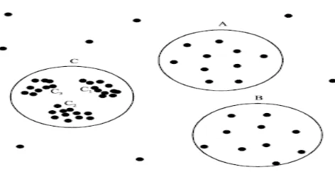
An important property of many real world data sets is that their intrinsic cluster structures are unable to be characterized by global density parameters. As a result, very different local densities may be needed to reveal clusters in different regions of the data space. For example, in the data set depicted in Fig. 1, it is impossible to detect the clusters A, B, C1, C2, and C3 simultaneously using one global density parameter. A global density-based decomposition would be needed for the clusters A, B, and C, or C1, C2, and C3. In the second case, the objects from A and B may be noise only [2].
Fig. 1 Density varied datapoints
Major headings are to be column centered in a bold font without underline. They need be numbered. "2. Headings and Footnotes" at the top of this paragraph is a major heading.
4. Proposed Methods
4.1 Method for determining different Eps’ values
To determine different range of Eps values automatically to identify the number of point processes (or clusters of different densities) including noise, we need to first draw a k-dist graph for all the points, for a given k i.e. k value will b entered by the user. Initially we compute the average of the distances of a point to all k of its nearest neighbors [3][6]. This is unlike VDBSCAN, where only the kth nearest neighbor is considered during the distance computation. The use of the K-dist plot structure enables efficient computation of k-nearest neighbors of a point, particularly for large data. The averaging allows a smoothing of the curve towards noise removal, for subsequent easier automated detection of density thresholds. We plot these averaged k-distances in an ascending order, to help identify noise with relative ease. We know that patterns corresponding to noise are expected to have larger k-distance values. The aim is to determine the “knees” for estimating the set of Epsparameters [3][6].
ISSN 2348 – 7968
plot. In short to find all possible Eps values we will have to calculate the slopes at regular interval and then find the difference between slopes values at the same regular interval. By setting certain threshold value we can get different Eps values automatically based on this threshold value while discarding those with higher thresholds.
Fig. 2 Average K-dist sorted plot
In general, it is very difficult to detect the first Eps values automatically, but it is relatively simple for a user to recognize this valley in a graphical representation. Obviously, the shape of the sorted k-distance plot and hence, the effectiveness of the proposed heuristic depends on the distribution of the k-nearest neighbor distances. For example, the plot will look more “stairs-like” if the objects are distributed regularly within clusters of very different densities or the first “valley” will be less clear if the densities of the clusters differ not much from the density of noise [3][6].
For datasets with widely varied density, there will be some variation, depending on the density of the cluster and the random distribution of points, but for points of the same density level, the range of variation will not be huge while a sharp change is expected to see between two density levels. Thus there will be several smooth curves connected by greatly variation ones [3]. If there are n (natural number n>1) different smooth curves in the k-dist plot, the dataset has n density levels. A dataset is of varied-density if it has several density levels and of n varied-density if it has n density levels. Specially, a dataset is of single-density if its density does not vary widely, or there is only one smooth curve in its k-dist plot. Figure 7 shows plotted k-dist graph for a given dataset with k value which will be specified by the user [3].
For points that are not in a cluster, such as noise points, the corresponding k-dist line rockets, connecting two smooth
curves which stand for two density levels. Line b and d in Figure 7 are such lines, which can be called level-turning lines. Line b connects line a and c, and line d connects c and e, while a, c and e stand for different density levelsb[3]. Note that line f shows the k-dists of outliers and is not a level-turning line for it does not connect two smooth lines. For different density levels Di, select suitable
Eps. For example, in Figure 7, there are three density levels. Line a shows the densest density level and e shows the sparsest one. Combine line a and b as a sub-k-dist plot to select Eps1, and then take line c and d as a sub-k-dist
plot for Eps2, e and f for Eps3 finally.
After determining the optimal number of different Eps values we need to start forming clusters starting from the lowest Eps value in the sorted k-dist graph, by sequentially execute DBSCAN for each of the Eps estimated considered in ascending order. The first estimate obviously corresponds to the denser cluster. Tagging the patterns in the already detected clusters as “visited”, we proceed towards larger values of k-distance while allowing DBSCAN to work on the still unvisited patterns only. In this manner we are able to effectively determine all clusters in a multi-density framework, in a decreasing order of density, with noise being modeled as the sparsest region [3][6].
So we need to adopt algorithm DBSCAN for each Epsi.
Before adopt DBSCAN for Epsi+1, mark points in clusters
corresponding with Epsi as Ci-t (t is a natural number),
which indicates that the points belong to the cluster t in density level i. Marked points will not be processed by DBSCAN again. Non-marked points after all the Epsi
process are recognized as outliers. And all the Ci-t are
displayed as the results [3][6].
4.2 Method for determining Minpts values
After determining the different Eps values, how to estimate the value of the MinPts is our urgent task. So firstly, the number of data objects in Eps neighborhood of every point in dataset is calculated one by one. And then mathematic expectation of all these data objects is calculated, which is the value of MinPts.
Minpts = 1/n
∑
=n
i
Pi
1Where pi is the number of points in Eps neighborhood of
ISSN 2348 – 7968
4.3 Method for finding value of ‘k’
To find the value of k automatically, consider a dataset with n points. First we will have to find out all the points average one to all other points distance to other points. Let’s consider one point and find distance to all the other points from it and average it to find the average distance [5].
)
1
(
2
)
,
(
tan
)
(
1−
=
∑
=n
Xi
Pi
ce
dis
Pi
d
n
i
Here,
d(Pi)=Average distance from Pi to all other points in the
data set.
We have to find out d(Pi) for all Pi.
Now we have to calculate avg(d). Which is the average of all d(Pi) which is required to find out the Target Point (Ti) .
n
Pi
d
d
avg
n
i
∑
==
1)
(
)
(
For every Pi in the datasets we will draw a circle and the
centre of the circle will be the points itself means Pi, and
the radius of each circle will be the avg(d). So area of each circle will be same. Here we conceive only the circumference of each circle. Here,
Pi=Subjective Point or Centre of the Circle
r =avg(d) (Radius of each Circles.)
For every circle we have to determine the closest point which is nearest to the circumference of each circle by the following equation.
min| (distance ( r – xi )) |
Xi is the point which has minimum distance from the
circumference of a particular circle for the corresponding Pi which is the centre of that circle. And for that Pi we
make Xi as a Target Point and tag as Ti .We have to find
out Ti for every Pi. Then we have to determine the position
of Ti relative to the Pi for that particular circle.
Ti(Pos)=Position of the Ti relative to the Pi of a particular
circle.
In this way we will determine the Ti(Pos) of Ti for all Pi in
the dataset. Next we have to determine the mode of Ti(Pos). That means we have to find out maximum
repeated Ti(Pos). If there is more than one mode then we
have to compute the mean of maximum repeated Ti(Pos)s
or modes. Mode of Ti(Pos) is basically our expected value
of parameter K in the K-dist plot [5].
5. Proposed Algorithm
Step 1: For each point calculate the distance to all the other points from it and average it to find the average distance as
)
1
(
2
)
,
(
tan
)
(
1−
=
∑
=n
Xi
Pi
ce
dis
Pi
d
n
i
Step 1.1: Find avg(d), Which is the average of all d(Pi).
n
Pi
d
d
avg
n
i
∑
==
1)
(
)
(
Step 2: For each Pi in the datasets, draw a circle with
centre as Pi and the radius as avg(d).
Step 2.1: For every circle determine the closest point which is nearest to the circumference of each circle using,
min| (distance ( r – xi )) |
where Xi is the point which has minimum distance from
the circumference.
Step 2.2: Mark for each Pi, Xi as the Target Point Ti.
Step 2.3: Calculate the position of Ti as Ti (Pos) relative to
the Pi for each particular circle.
Step 2.4: Determine the mode of Ti (Pos) i.e. find out
maximum repeated Ti (Pos).
Step 2.5: If there is more than one mode then compute the mean of maximum repeated Ti (Pos)s.
Step 2.6: Mode of Ti (Pos) is the value of K which is the
number of neighbourhood points.
Step 3: Calculate the average of the distances of every point to all Kof its nearest neighbors.
Step 4: Sort them in ascending order.
Step 5: Draw the averaged K-distances plot in an ascending order.
Step 6: Compute the slope values at regular interval. Step 7: Compute difference between slope values at regular interval.
Step 8: If the difference is 10% times higher than previous slope value then consider it as Epsi (i=1,2,…,n)value.
Step 9: ElseIf the difference is 25% times higher than previous slope value then ignore it and consider it as a noise points.
Step 10: For each Epsi (i=1,2,…,n) value do,
Step 10.1: Calculate for each point in the dataset the number of data points in Eps neighborhood.
Step 10.2: Compute MinPtsi (i=1,2,…,n) value for each
Epsi (i=1,2,…,n) value using following,
Minptsi = 1/n
∑
=
n
i
Pi
1where Pi (i=1,2,…,n) is the number of points in Eps
ISSN 2348 – 7968
Step 11: For each Epsi (i=1,2,…,n) and MinPtsi
(i=1,2,…,n) value,
Step 11.1: Use parameters as Eps = Epsi and MinPts =
MinPtsi,
Step 11.2: Adopt DBSCAN algorithm.
Step 11.3: Mark points in clusters corresponding with Epsi
as Ci..
Step 12: Repeat step 11 and adopt DBSCAN algorithm with other Epsi and MinPtsi value ignoring the marked
points.
Step 13: Display all the clusters Ci, non-marked points are
outliers.
5. Conclusion
Among all clustering methods, density-based clustering algorithm is one of powerful tools for discovering arbitrary-shaped clusters in large spatial databases. In this paper, I presented the literature work in the field of density based clustering along with my proposed methods and algorithm to enhance the DBSCAN algorithm. There are vast ranges of Clustering techniques being proposed over the period of time and every technique has some advantages to other along with some disadvantages. Most of the clustering techniques do not scale well with large data sets and more so when the dimensionality of the data is large. Almost all of the well-known clustering algorithms require input parameters which are hard to determine but have a significant influence on the clustering result. Furthermore, for many real-data sets there does not even exist a global parameter setting for which the result of the clustering algorithm describes the intrinsic clustering structure accurately. In short there are no algorithms which detect clusters automatically. Usually, user does not know enough information to determine the input parameters. Therefore, obtaining reasonable clustering results requires testing large different initializations. Minimizing input parameters will certainly be very useful in reducing the errors introduced by human interference. DBSCAN algorithm requires two input parameters called Eps and MinPts, hence leading to above mention shortcomings which were overcome somewhat by OPTICS and various other algorithms, but main improvement was achieved by VDBSCAN algorithm which is one of the most efficient algorithms for creating clusters from dataset of varying density. However even this algorithm has shortcomings of lot of user interaction and making user to select the best value of K, thus leading to same problem as before. So through this paper I have presented methods to select the range of Eps and MinPts value automatically and algorithms with both parameters automatic to find density varied clusters.
References
[1] M Ester, H-P. Kriegel. J. Sander, and X, Xu. 1996. “A density-based algorithm for discovering clusters in large spatial databases”. KDD’96.
[2] M. Ankerst, M. Breunig, H.P. Kriegel, and J. Sandler. “OPTICS: Ordering Points to to Identify the Clustering Structure”; proceedings of the Int. Conf on Management of Data, pp. 49-60, 1999.
[3] zeng Liu, Dong Zhou, Naijun Wu, ”Varied Density Based Spatial Clustering of Application with Noise”, in
proceedings of IEEE Conference ICSSSM 2007 pg 528-531.
[4] Adriano Moreira, Maribel Y. Santos and Sofia Carneiro, “Density-based clustering algorithms – DBSCAN and SNN”, 2005.
[5] Hongfang Zhou, Peng Wang, Hongyan Li, “Research on Adaptive Parameters Determination in DBSCAN Algorithm”, Journal of Information & Computational Science 9: 7 (2012).
[6] Sushmita Mitra1 and Jay Nandy “KDDClus: A Simple Method for Multi-Density Clustering”, 2010.
[7] M.Parimala, Daphne Lopaz, N.C. Senthilkumar, “Survey on Density based Clustering Algorithm for mining large spatial databases”, IJAST 2011.
[8] Pang-Ning Tan, Michael Steinbach, Vipin Kumar, “Introducing to Data Mining”, Pearson Education Asia LTD, 2006.
[9] Jason D. Peterson, “Clustering overview”,
http://www.cs.ndsu.nodak.edu/~jasonpet/CSCI779/Clu stering.pdf.
[10] M. Ester, H. P. Kriegel, J. Sander, and X. Xu. “A density based algorithm for discovering clusters in large spatial data sets with noise”; in 2nd International Conference on Knowledge Discovery and Data Mining, pp. 226–231,1996.
[11] Sheikholeslami G., Chatterjee S., Zhang A.: “WaveCluster: A Multi-Resolution Clustering Approach for Very Large Spatial Databases”, Proc. 24th Int. Conf. on Very Large DataBases, New York, NY, 1998, pp. 428 - 439.
[12] Hattori K., Torii Y.: “Effective algorithms for the nearest neighbor method in the clustering problem”,
Pattern Recognition, 1993, Vol. 26, No. 5, pp. 741-746.
[13] Mariam Rehman, Syed Atif Mehdi, "Comparison of Density-based Clustering Algorithms", 2006.
Kedar Sawant Completed B.E.(I.T.) in June, 2009 and M.E. (C.S.E.) in