Robust Stability Based Pid-Controller
Design of D.C. Servo Plant with Time-Delay
and Additive Uncertainty
Anwar S. Siddiqui
1, Aziz Ahmad
2Professor, Dept. of Electrical Engineering, F/o Engineering & Technology, Jamia Millia Islamia, India1 Research Scholar, Dept. of Electrical Engineering, F/o Engineering & Technology, Jamia Millia Islamia, India2
ABSTRACT: The area of control system engineering that mainly deals in obtaining the robustness of system in the existence of uncertainties is known as robust control. In this paper, a graphical design method is developed for obtaining the entire range of PID controller gains that stabilize a D.C. servo plant robustly with the existence of time delays and additive uncertainty employed. This method of design mainly works on the frequency response of the system, which can provide to decrease the complexities implicated in servo plant modeling. In fact in the real time processes, the time-delays and parametric uncertainties are more or less always present, that makes our controller design method crucial for process control. We have used this graphical method of design to find the robust stability of a DC servo plant model with a delay in communication and additive uncertainties. The results were found satisfactory and robust stability has achieved for the said model.
KEYWORDS: PID controller, robust control, DC servo plant, Time delay, Uncertainty, Stability.
I. INTRODUCTION
Presently the PID controllers are most effectively and widely used in the process control industries. The PID controller structure basically makes simple to control the process plant output. Graphical methods for designing PID controllers which operates effectively and optimally are simple, and these methods are very essential for process industries.
Robust control is concern with acquiring control systems which are indifferent to plant/model uncertainty or mismatch. In order to acquire the plant stability with respect to time uncertainties and time delays, wide research has been carried out in the designing methods of the controllers. This paper presents a design based on graphical method to get gains of the PID controller in order to achieve a robust stability, considering with parametric uncertainties and time delays for arbitrary order plants. Let us consider a model having an additive uncertainty, in order to acquire the whole set of uncertainty. The design methodology of H∞ controller is considered to find the uncertain plant remains stable for the whole set of
uncertainty.
Proposed design method lower down the complexities of plant modeling in the frequency domain application. This method of controller design considering with parametric uncertainties and time delays is then subjected to a DC servo plant model. Example of the DC servo plant shows that there will be assured robust and closed loop stability with the PID controller gains. Most of the initial works done in this field is mainly dedicated on finding that PID controllers which stabilizes a nominal plant model.
Hermite-Biehler theorem is generalized and used by Bhattacharyya and their colleagues in order to find out all stabilizing PID controllers considering with time delay for systems [6 to 8].
Reference [10 to 13] shows some techniques in order to find out all those achievable PID controllers that satisfied complementary and weighted sensitivity, robust stability and performance constraints and those PID controllers that stabilized an arbitrary order system.
II. PROPORTIONAL - PLUS – INTEGRAL - PLUS DERIVATIVE CONTROLLERS
In 1939 PID controller was first to be placed in the market and till now in the process control, this controller is most broadly used. More than 90% of the controllers are PID controllers and its advanced version that are used in the process industries; this is an investigation which is carried out in Japan in 1989. These controllers are quite familiar because derivative action is sensitive to the noise measurement. The main tool of the PID controller is the “PID control” which is the method of feedback control. Figure (1) indicates the fundamental structure of conventionally used feedback control systems. Below figure represents the process of the plant which has to be controlled.
Set-point value (r) has to be followed by process output variable (y), this is the purpose of control. This purpose can be achieved if the manipulated variable (u) modify at the command of the controller. Let us take an example of a process plant, assume some liquid is heated in a heating tank by the burning of fuel gas for some desired temperature. Temperature of the liquid is y (i.e. output variable of the process plant) and the flue gas flow is u (i.e. manipulated variable). Any factor that influences the output variable of the process except manipulated variable is a disturbance. It is assumed that the manipulated variable is added by a single disturbance in the Figure (1). However in some cases, a major disturbance enters the process or there is a need for considering the multiple disturbances. e = r – y, this equation defines error „e‟.
u (the manipulated variable) determined by the controller C(s) computational rule based on its input data is the error (e) in the given figure (1).
One more thing which has to be noticed in Figure (1) is that it is assumed that detector measures the process output variable (y), the controller input can be considered as exactly being equal to y, with adequate accurateness instantly, which is not clearly mentioned here.
Fig.(1) PID Controller
Hence, the PID controller can be understood as a controller that takes into consideration: the past, the present and the future of the error. Gc(s) known as gain or transfer function of the PID controller can be given by:
GC(s) = KP (1+
1
𝑠𝑇𝑖+Td s) ………... (1)
Gc(s)=KP+
𝐾𝑖
𝑠+Kd s ...(2)
Where,
Controller proportional gain is indicated by KP;
Controller integral gain is indicated by Ki; and
Controller derivative gain is indicated by Kd;
The controllers can provide control action designed for specific process requirement by tuning the gains of these PID controllers [3].
III. THE CONCEPTS OF ROBUST CONTROL
Loop shaping technique is an important classical controller design method [1]. The classical feedback control methods were extended to a more renowned method based on shaping closed-loop transfer functions such as the weighted sensitivity function during the 1980‟s. These developments led to a more deep understanding of robust control concepts. An extensive research had been made during this period of time covering the number of techniques for modern robust control concepts and its uses to real-world systems [3].
IV. UNCERTAINTY MODEL
If differences in between the model of the system, used in designing a controller and of the actual system is not sensitive to a control system than such system is known as robust control system. These types of differences simply represent uncertainty in model or model/plant mismatch.
Furthermore, the key plan of the robust control is to verify whether the design specifications are met for the “worst-case” uncertainty [1]. The following approach to check robustness of the system.
1. Nominal stability of system should be checked.
2. Find out the Uncertainty Set: a mathematical representation of the system plant model uncertainty have to be determined.
3. Robust Stability (RS) Verification: Determine whether the system remains stable for all system plants in the uncertainty system.
4. Robust Performance (RP) Verification: If RS is satisfied; determine whether the performance specifications are met for all system plants in the uncertainty system.
A general block diagram representation of a one degree-of-freedom feedback control system is shown in figure (2), [1]. Where, r is the reference input, u is the controlled input to the plant, y is the actual plant output and d is the disturbance signal and n is the noise signal. The plant model, disturbance model and controller gains are represented by G, Gd, and K respectively.
The main objective of a control system is to make the output y must act in a desired manner by manipulating u such that the control error remains very small in spite of the disturbances present in the system. The system output can be denoted as:
Y = G(s)u + G(s)d………...(3)
Fig.(2) Feedback control system with one degree-of-freedom [2].
V. TIME-DELAY SYSTEMS
It is to be found that most of the real-time systems have time-delay associated with them. There may be one or more of the following reasons of Time delay origination [2]:
1. System variables measurement.
2. Physical properties of the apparatus used in the system. 3. Transport delay in the signal transmission.
The effect of the time delay on a system depends on the size of the delay and system characteristics. Systems where the time delay plays a vital role are control, economic, political, biological, and environmental systems. A few examples include speed control of an engine, a cold rolling mill, spaceship control, unman-vehicle and hydraulic systems [2]. A block diagram representation of a cascade time delay system illustrated in figure (3).
VI. UNCERTAINTY AND ROBUST STABILITY FOR SINGLE-INPUT -SINGLE-OUTPUT (SISO) PLANT SYSTEMS [16]
In order to design the control system, a robust control system always strives to remain insensitive towards the differences between the actual system and the model of the system.
In this paper, the primary objective is to determine the set of PID controllers that will guarantee robust stability for any arbitrary order SISO plant in the presence of time-delay and additive uncertainties.
As mentioned in [1], the origins of model uncertainty are as follows: 1. Parameters in the linear model that are approximately known
2. Parameters that vary due to nonlinearities or changes in the operating conditions 3. Measurement devices often have imperfections
4. At high frequencies the structure and model order is often not known
5. Controller implemented may differ from the one obtained by solving the synthesis problem
Fig.(4) Plant with additive uncertainty [1] Based on the above criteria, the main classes of model uncertainties are as follows.
VII. PARAMETRIC UNCERTAINTY
In the Fig.4, GΔ(s) represented the perturbed plant which includes ΔA (s), which is any stable transfer function such that І
ΔA (jω) І≤1, ∀ ω. In the frequency domain we can represent these transfer functions as:
jω = Re ω + jIm(ω) K jω = Kp+
Ki
jω+ Kdjω WA(jω) = AA(ω) + jBA(ω)
∥ WA jω K jω S(jω) ∥∞≤γ...(4)
If this condition is fulfilled and γ=1, then
S jω = 1
1+Gp jω K(jω) ...(5)
WA jω K jω S jω = ⎸WA jω K jω S jω ⎹ej∠WA jω K jω S(jω) WA jω K jω S jω ejθA ≤γ∀ω
Or WA jω K jω
1+Gp jω K jω e
jθA ≤γ∀ω ...(6)
Where, θA= −∠WA jω K jω S jω
P ω,θA,γ = 0
Where the system characteristic polynomial 𝐏 𝛚, 𝛉𝐀, 𝛄 can be written as: P ω,θA,γ = 1 + Gp jω K jω −
1
γ WA jω K jω ejθA ejθA = cosθ
A+ jsinθA P ω,θA,γ = 1 + Re ω+ jIm(ω) Kp+
Ki
jω+ Kdjω − 1
γ AA(ω) + jBA(ω) Kp+ Ki
jω+ Kdjω cosθA+ jsinθA
For 𝛄 →∞,
𝐗𝐑𝐩Kp+𝐗𝐑𝐢Ki+𝐗𝐑𝐝Kd=0 ...(A)
𝐗𝐈𝐩Kp+𝐗𝐈𝐢Ki+𝐗𝐈𝐝Kd=0 ...(B)
XR p=-ω Im ω +1
XR i= Re ω +1
γ AAcosθA− BAsinθA ...(8)
XR d=-ω2 Re ω +1
γ AAcosθA− BAsinθA ...(9)
XI p=ω Re ω +1
γ AAcosθA− BAsinθA ...(10)
XI i= Im ω +1
γ AAsinθA+ BAcosθA ...(11)
XI d=-ω2 Im ω +1
γ AAsinθA+ BAcosθA ...(12)
VIII. PID CONTROLLER DESIGN IN (KP,KD) PLANE FOR CONSTANT KI
The transfer function model of the DC servo plant is represented as: G(s)= 𝟓𝟑.𝟐𝟕
𝐬(𝐬+𝟑𝟔.𝟐)
The boundary for 𝐏 𝛚, 𝛉𝐀, 𝛄 = 𝟎 for the (Kp, Kd) plane for a fixed value of Ki=𝐊i found using above equations (A) and
(B), which can be rewritten as
XR p XR i XI p XI i
Kp
Kd =
0 − XRiKi
−ω− KIiKi
…………...(13) Solving equation (13) for all 𝛚 ≠ 𝟎 and 𝛉𝐀 𝜖 0, 2𝜋, we obtain the controller gains as,
Kp ω,θA,γ =
−Re ω −1γ AAcosθA− BAsinθA X(ω)
Kd ω,θA,γ = Ki
ω2+
Im ω +1γ AAsinθA+ BAcosθA
ωX(ω)
Where,
X(ω) = |Gp jω |2+ 1
γ|WA jω |2+ 2
γ Re ω AAcosθA− BAsinθA + Im ω AAsinθA+ BAcosθA
Equation (13) can be rewritten as
−ωα(ω) −ω2β(ω)
ωβ(ω) −ω2α(ω) Kp Kd
= 0 − XRiKi
−ω− KIiKi
Where,
α(ω)= Im ω +1
γ AA(ω) sinθA+ BA(ω)cosθA
β(ω)= Re ω +1
γ AA(ω)cosθA− BA(ω)sinθA
For ω= 0 a solution may exist if Ki= 0. Solving
−α(0) 0
β(0) 0 Kp Kd
= 0 −1
We obtain –α 0 Kp = 0 andβ 0 Kd = −1.
For additive uncertainty weight the following form is selected:
𝑤 =
𝑀
ℎIX. RESULTS OF THE ROBUST CONTROLLER IN DIFFERENT PLANES:
Fig.(5) Additive weight representation The fig (5) shows the graph of additive uncertainties weight functions.
Fig.(6) Nominal stability boundary and robust stability region for Kp and Ki values
In fig. (6) the regions of nominal stability boundary and robust stability region for Kp and Ki values are illustrated.
Fig.(7) Magnitude of WA jω K jω S jω for a point inside the robust stability region
Fig. (7) shows the frequency response of the robust controller with the plant. It also satisfies the condition of the robustness of the system.
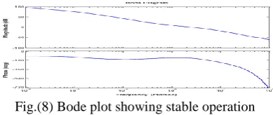
Fig.(8) Bode plot showing stable operation
In fig.(8) gives the information of the system‟s stable operation as per the bode plot criterion.
The values of the Kp and Ki taken outside the nominal boundary as shown in fig. (9). For these values of Kp and Ki the system operations becomes unstable.
Fig.(10) Magnitude of WA jω K jω S jω for a point outside the robust stability region
Unstable Response of the system shown in fig. (10), where the criterion is not meet.
Fig.(11) Bode plot showing the unstable operation The Bode plot for unstable operation of the system shown in fig. (11).
X. RESULTS DISCUSSION
The results are obtained shown in figures 5-11. In fig.6 additive uncertainty weight assign to the controller is shown fig.6 showing the points of operation within robust stability region and nominal stability region shown by red line. Within the points considered stability criterion i.e magnitude of WA jω K jω S jω <1 satisfied as shown in fig.7. For these points
fig.8 showing the Bode plot with stable operation. Now we have considered two points, one within nominal stability region but outside of robust stability region and one point outside of nominal stability region as shown in fig.9. Result obtained in fig.10 does not satisfied the magnitude of stability criterion WA jω K jω S jω <1. Therefore, Bode plot in fig.11 showing
the unstable operation. Similar results are obtained for (Kd, Kp ) and ( Kd, Ki) planes.
XI. CONCLUSION
A graphical design method for obtaining all PID controllers that satisfied a robust stability constraint for a DC servo plant with time delay and uncertainties has coded in MATLAB. Observing the results it can be concluded that the PID controllers selected from the robust stability regions in the (Ki , Kp ) plane satisfy the robust stability constraint for the DC servo plant model. Using Bode plot‟s gain and phase margin Robust stability is founded. Similar results are found for (Kd, Kp) and ( Kd, Ki) planes. It is concluded that all the Points within the robust stability region are always stable but all the points within the nominal stability region need not necessarily be always stable for different planes.
REFERENCES
[1] Skogestad, S. and I. Postlethwaite, Multivariable Feedback Control, John Wiley & Sons Ltd., Baffins lane, Chicester, West Sussex PO19 1UD, England, 2001, Chapters 2, 7, pp. 15-62, pp. 253-290.
[2] Sujoldzic S. and J. M. Watkins, “Stabilization of an arbitrary order transfer function with time delay using PID controller,” Proceeding of IEEE Conferance on Decision and Control, Vol. 45, December. 2005.
[3] Dorf, Richard C. and Robert H. Bishop, Modern Control Systems, 9th edition, Prentice–Hall Inc., New Jersey-07458, USA, 2001, Chapters 1, 5, pp. 1-23, pp. 173-206.
[4] H. Bevrani, Robust Power System Frequency Control, Springer Science + Business Media, LLC, 233 Spring Street, New York, NY-10013, USA, 2009, Chapter 2, pp.15-30.
[5] Bhattacharyya, S. P., Chapellat, H., and L.H. Keel, Robust Control: The Parametric Approach, Prentice Hall, N.J., 1995.
[7] Ho., K.W., Datta, A., and S.P. Bhattacharya, “PID stabilization of LTI plants with time-delay,” Proc. 42nd IEEE Conferance on Decision and Control, Maui, Hawaii, 2003.
[8] Bhattacharyya, S.P. and L.H. Keel, “PID controller synthesis free of analytical methods,” Proceeding of IFAC 16th Triennial World Congress, Prague, Czech Republic, 2005.
[9] Sujoldzic, S. and J. M. Watkins, “Stabilization of an arbitrary order transfer function with time delay using PI and PD controllers”, Proceeding. of American Control Conference, June 2006, pp. 2427-2432.
[10] Emami, T. and J.M. Watkins, “Weighted sensitivity design of PID controllers for arbitrary-order transfer functions with time-delay,” Proceeding of the IASTED International Conf. on Intelligent Systems and Control, November 2008, pp 20-25.
[11] Emami, T. and J.M. Watkins, “Robust stability design of PID controllers for arbitrary-order transfer functions with uncertain time delay,” South eastern Symposium on System Theory University of Tennessee Space Institute, March 2009, pp. 184-189.
[12] Emami, T. and J.M. Watkins, “Complementary sensitivity design of PID controllers for arbitrary-order transfer functions with time delay,” Proc. of 2008 ASME Dynamic Systems and Control Conf., October 2008.
[13] Emami, T. and J.M. Watkins, “Robust performance characterization of PID controllers in the frequency domain,” WSEAS Transactions Journal of Systems and Control, Vol. 4, No. 5, May 2009, pp. 232-242.
[14] Zavarei, M. M. and M. Jamshidi, “Time-Delay Systems: Analysis, Optimization and Applications”, Elsevier Science Publisher, Amsterdam, Netherlands, 1987, Chapter 1, pp. 1-15.
[15] Graham, Goodwin C., Graebe, Stefen F., and Mario E. Salgado, “Control System Design,” online URL:http://csd.newcastle.edu.au/chapters/Fig1_1.png, DateRetrieved: March 2010.
[16] Singh Gursewak and gagandeep Kaur, “Robust Stability of LTI (SISO) system with System gain (A) under uncertainty set using PID controller”, International Journal of Advances in Computing and Information Technology, 2012. 2, pp .128-143.
[17] Vineet Kumar A. P. Mittal, “Parallel Fuzzy P+Fuzzy I+Fuzzy D Controller: Design and Performance Evaluation”, International Journal of Automation and Computing, 7(4), November 2010, 463-471.
BIOGRAPHY
Prof. Anwar Shahzad Siddiqui obtained his B.Sc. Engg. (Electrical Engineering) and M.Sc. Engg. (Power System and Electrical Derives) degrees from AMU, Aligarh, both with Honors in 1992 and 1994 respectively. He earned his Ph.D. degree from Jamia Millia Islamia (Central University) New Delhi, India in 2001.He has been teaching and guiding research in Electrical Engineering for about one and half decade at AMU, Aligarh; JMI, New Delhi and BITS Pilani-Dubai Campus. His research interests include Control systems Engineering, Power systems and Applications of Artificial Intelligence Techniques in Control Systems as well as Power systems. He has more than 60 research papers published in refereed international and national journals and conferences of repute.