Performance Evaluation of Adaptive Line
Enhancer Implementated with LMS, NLMS and
BLMS Algorithm for Frequency Range
3-300Hz
Shobhit Agarwal 1 , Raghu Raj Singh2, Namrta Dadheech3, Sarita Chauhan4
B.Tech Student, Dept. of ECE, M.L.V Textile and Engineering College, Bhilwara, Rajasthan,India1,2,3
Assistant Professor, Head of Dept. of ECE, M.L.V Textile and Engineering College, Bhilwara, Rajasthan,India4
ABSTRACT
:
In this paper, an adaptive line enhancer using LMS,BLMS and NLMS algorithm has been simulated for low electromagnetic frequency range (ELF&SLF-3to300Hz.) range using MATLAB software. Firslty,Sinusoidal wave is corrupted with the white noise then we have adaptively filtered corrupted wave over the required frequency range, but in the paper only 60Hz result have been shown. Later on , the adaptive behaviour of the algorithms is analyzed and performance criteria are used in the study of these algorithms are : the minimum mean square error(MSE) and Signal to noise ratio. The paper compares a performances of ALE using LMS, NLMS and the BLMS algorithms for a given range. Different SNR ratio level is obtained as the step-size is changes, their relative SNR result is shown.
KEYWORDS: Adaptive Line Enhancer (ALE), Least Mean Square (LMS), Block LMS (BLMS),Normalised least mean square(NLMS),Extremely low frequency(ELF),Super low frquency(SLF),MSE(mean squared error)
I.INTRODUCTION
Adaptive filter is that it uses the filter parameters of a moment ago to automatically adjust the filter parameters of the present moment, to adapt to the statistical properties of unknown signal and noise , in order to achieve optimal filter. Adaptive algorithms based on the least mean square (LMS) algorithm, normalized least mean square (NLMS), and block least mean square(BLMS) processing algorithms are applied to the adaptive filter technology to the noise, and through the simulation results prove that its performance is usually much better than using fixed digital filter.
Most of the submarine communication uses the very low frequency i.e electromagnetic waves in the ELF and SLF frequency ranges (3–300 Hz) can penetrate seawater to depths of hundreds of meters, allowing communication with submarines at their operating depths. Hence using, the concept ALE on the signals that are affected by white noise, received in submarine can be filtered easily.
II. LITERATURE SURVEY
ALE uses only a single sensor to detect the target signal buried in noise, though it may use the same adaptive. The ALE is in fact a degenerated form of ANC, consisting of a single sensor and delay z-Δ to produce a delayed version of d(n), denoted by x(n), which de-correlates the noise while leaving the target signal component correlated. Ideally, the output
y(n) of the adaptive filter in the ALE is an estimate of the noise-free input signal. Hence, the ALE capability to extract the periodic and stochastic components of a signal can also be known as an adaptive self-tuning filter (Widrow et al. 1985, Campbell et al. 2002).The ALE becomes an interesting application in noise reduction because of its simplicity and ease of implementation. However, to obtain the best performance in its computational process, the optimal approach is to execute ALE on a better convergence rate of adaptive algorithm with a less complex adaptive filter structure algorithm as the ANC.
Electromagnetic waves in the ELF and SLF frequency ranges (3–300 Hz) can penetrate seawater to depths of hundreds of meters, allowing communication with submarines at their operating depths. Building an ELF transmitter is a formidable challenge, as they have to work at incredibly long wavelengthsDue to the technical difficulty of building an ELF transmitter, the U.S., Russia and India are the only nations known to have constructed ELF communication facilities. Until it was dismantled in late September 2004, the American Seafarer, later called Project ELF system (76 Hz), consisted of two antennas, located at Clam Lake, Wisconsin (since 1977), and at Republic, Michigan, in the Upper Peninsula (since 1980). The Russian antenna (ZEVS, 82 Hz) is installed at the Kola Peninsula near Murmansk. It was noticed in the West in the early 1990s. The Indian Navy has an operational ELF communication facility at the INS Kattabomman naval base to communicate with its Arihant class and Akula classsubmarines
III.ADAPTIVE LINE ENCHANCER
Adaptive line enhancer (ALE) is used in many signal processing fields for its capability of tracking a signal of interest. The main advantage of it is that it does not require any reference signal to eliminate the noise signal.
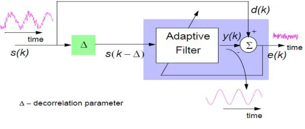
Fig. 1, show the adaptive filter setup, where s(k) , d(k) and e(k) are the input, the desired and the output error signals, respectively. The vector h(n) is the Mx1 column vector of filter coefficient at time k , in such a way that the output of signal, y(k) , is good estimate of the desired signal, d(k). This filter is an adaptive filter whose tap weights are controlled by an adaptive algorithm. Thus ALE refers to the case where a noisy signal, x(k),consisting of a sinusoidal component and the requirement is to remove the noise part of the signal. As a result, the predictor can only make a prediction about the sinusoidal component and when adapted to minimize the instantaneous squared error output, e(k), the line enhancer will be a filter optimized (the Wiener solution) or tuned to the sinusoidal component.
Figure.1-Basic Adaptive line enchancer
IV.ADAPTIVE ALGORITHM
approximated gradient. For the LMS algorithm it is necessary to have a reference signal d[n] representing the desired filter output. The difference between the reference signal and the actual output of the transversal filter is the error signal which is given in the equation (1)
y(n)=wt(n)x(n) Filter Output ...(1)
e(n) = d(n)-y(n) Error ...(2)
w(n)=[w0(n) w1(n)..wM1(n)]t Filter Coeffcients at time n ...(3)
x(n)=[x(n) x(n1) x(n2).x(nM+1)]t Input Data ...(4)
where the filter coeffcients are calculated using the equation w(n+1) = w(n) + 2µe(n)x(n) ...(5)
Considering as the step size(µ). The algorithm at each iteration requires that x(n),d(n) and w(n) are known. As the step size decreases, the convergence speed to the optimal values is slower. This also implies that, the LMS algorithm is a stochastic gradient algorithm if the input signal is a stochastic process. 2)Block LMS
:-
In this method, the filter coefficients are held constant overeach block of the input signal. The filter output y(n) and errorsignal e(n) are calculated using filter coefficients of that block. Then, the filter coefficients are updated at the end of each block using an average of the L gradient estimates over that block. For kth block, the output of the filter is described as, Y(kL + l) = .x(Kl+1)………… (5)and the error signal is given by, e(kL+ d)=d(kL+ l)- y(kL + l…….. (6)
where, L is the block length and d(n) is the desired signal. The weight update equation of the kth block, w(k+1)L =wkL+µ/L( e(kL + 1)x(kL + 1))…(7) 3)Normalised LMS-The main drawback of the "pure" LMS algorithm is that it is sensitive to the scaling of its input. This makes it very hard to choose a learning rate μ that guarantees stability of the algorithm. The Normalised least mean squares (NLMS) filter is a variant of the LMS algorithm that solves this problem by normalising with the power of the input. NLMS algorithm summary: Parameters: P = filter order μ = step size Initialization: ĥ (0) = 0 Computation: For n = 0, 1, 2... X(n) = [x(n), x(n - 1), …, x(n – p + 1)]T ………(8)
e(n) = d(n) – ĥ H(n) X(n) ………(9)
ĥ(n+1) = ĥ(n) + μ ∗( ) ( ) ( ) ( )...(10)
V. MEAN SQUARED ERROR
In this portion, we plot the error obtained from the equation 2,6 &9.Firstly, error is squared and then, plotted with respect to simulation time and finally response obtained is smoothen. Smoothing is done by moving average filter that smoothes data by replacing each data point with the average of the neighboring data points defined within the span
.
VI. RESULT AND DISCUSSION
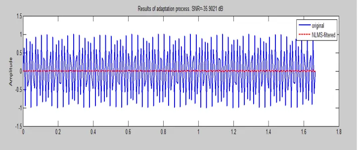
from different algorithms are shown in figure. Here Filtered signal is of 60Hz (Shown in fig.2,3,4) The order of the filter was set to M=16.Similarly, signal at other frequency can also be filtered and will produce same SNR ratio, since change in frequency doesn’t alter the power of signal.
Fig. 2 LMS filtered output at 60hz Blue colour wave represent original signal and red colour wave shows LMS filtered output
Fig. 3 BLMS filtered signal at 60hz. Blue colour wave represent original signal and red colour wave shows BLMS filtered output
Secondly, we change the value of step-size or convergence factor and then observe the change in SNR values of filtered output,as equations 1,5 & 9.Choosing the step size is completely a hit trail method.
Below given table shows the value of SNR obtained at different stepsize
Table1-SNR obtained at different step-size for LMS,NLMS,BLMS
In Table 1, negative value represent,that power of error signal is greater than information signal. This is possible since input signal is of low frequency.
Given below graph represent squared error graph at the step size of 0.01 with respect to simulation time.
Fig.5-BLMS mean squared error
Fig.6-LMS mean squared error
Fig.7-NLMS squared mean error
From Square mean(Fig.5,6,7)error plot we can say that error is quite near to zero and the constant error corresponds that the system is converging. In addition to the algorithm, the step size and filter length of an adaptive filter also affect the convergence speed. The learning curve of an adaptive filter gradually converges to zero and becomes steady at an MSE value of the error signal e(n).The difference between that MSE value and zero is known as the steady state error. An optimal adaptive filter typically has a small steady state error. You can minimize the steady state error by adjusting the step size and filter length of the adaptive filter
VI.CONCLUSION
For the low EMW(3-300hz), we can conclude that NLMS’s performance is much better then LMS and BLMS.If we consider the table then at step size 0.007 we can obtained best result for all the algorithm.SNR is highly dependent on the step size so, we have to choose such that it produces good result and even take less convergence time.
REFERENCES
[1]S.Arunkumar, P.Parthiban, S.Aravind Kumar-Implementation Of Least Mean Square Algorithm For Sinusoidal And Audio Denoising Using Fpga-Vol. 2, Issue 12, December 2013
[2] K. Prameela, M. Ajay Kumar, Mohammad Zia-Ur-Rahman and Dr B V Rama Mohana Rao-Non Stationary Noise Removal from Speech Signals using Variable Step Size Strategy
[3] Simon Haykin, “Adaptive Filter Theory”, Prentice Hall, 1996
[4] "Navy gets new facility to communicate with nuclear submarines prowling underwater". The Times of India31 July 2014.
[5] Yuu-Seng Lau, Zahir M. Hussian and Richard Harris, “Performance of Adaptive Filtering Algorithms: A Comparative Study”, Australian Telecommunications, Networks and Applications Conference (ATNAC), Melbourne, 2003.
[6]Manoj Sharma “Acoustic Echo Reduction Using Adaptive Filter:A Literature Review”, MIT International Journal of Electrical and Instrumentation Engineering, Vol. 4, No. 1, January 2014, pp. 7–11 ISSN 2230-7656 © MIT Publications
[7] Ying He, et. al. “ The Applications and Si mulation of Adaptive Filter in Noise Canceling”, 2008 international Conference on Computer Science and Soft ware Engineering, 2008, Vol.4, Page(s): 1 – 4.