Image Segmentation Using Iso-perimetric graph Theory and Its Comparative Analysis

Image Segmentation Using Iso-perimetric

graph Theory and Its Comparative Analysis

Amit Dikholkar1, Kuldeep Pande2, Abhishek Zade3, Deepika Sagne4, Aasawari Paturkar5

Department of Electronics Engineering, Yashwantrao Chavan College of Engineering, Nagpur, India123 Department of Electronics Engineering, Yashwantrao Chavan College of Engineering, Ramdeobaba College of

Engineering, Nagpur, India 4

Department of Electronics Engineering, Yashwantrao Chavan College of Engineering, Shri Datta Meghe Polytechnic,

Nagpur, India 5

ABSTRACT: - Graph cuts proved to be a useful multidimensional optimization tool which can enforce piecewise smoothness while preserving relevant sharp discontinuities. This paper is mainly intended as an application of isoperimetric algorithm of graph theory for image segmentation and analysis of different parameters used in the algorithm like generating weights, regulates the execution, Connectivity Parameter, cutoff, number of recursions,. We present some basic background information on graph cuts and discuss major theoretical results, which helped to reveal both strengths and limitations of this surprisingly versatile combinatorial algorithm, further algorithm results are compared with Berkeley’s Data base on two points PSNR(Peak Signal to Noise Ratio) & RI (Rand Index)

KEYWORDS: - graph theory, image partitioning, Isoperimetric algorithm, connectivity, PSNR, RI, Berkeley’s Database

I. GRAPH THEORY FOR IMAGE PARTITIONING

Graph processing algorithms have become increasingly popular in the context of computer vision. Typically, pixels are associated with the nodes of a graph and edges are derived from a 4- or

8-connected lattice topology. Some authors have also chosen to associate higher level features with nodes. For purposes of importing images to space variant architectures, we adopt the conventional view that each node corresponds to a pixel. Graph theoretic algorithms [1] often translate naturally to the proposed space-variant architecture. Unfortunately, algorithms that employ convolution (or correlation) implicitly assume a shift invariant topology. Although shift-invariance may be the natural topology for a lattice, a locally connected space-variant sensor array (e.g., obtained by connecting to K-nearest-neighbors) will typically result in a shift-variant topology. Therefore, a reconstruction of computer vision algorithms for space-variant architectures requires the use of additional theory to generalize these algorithms.

II. ISO-PERIMETRIC ALGORITHM

2.1 Iso-perimetric Problem

Graph partitioning has been strongly influenced by properties of a combinatorial formulation of the classic isoperimetric problem: For a fixed area, find the region with minimum perimeter.

Defining the isoperimetric constant I of a manifold as:

inf(|

S

|)

I

V



where S is a region in the manifold, V denotes the volume of region S, |S| is the area of the boundary of region S, and I is the infimum of the ratio over all possible S. For a compact manifold volume of region S is less than or equal to 50 % of total volume and for a non-compact manifold, volume of the region < ∞.

We show in this paper that the set (and its complement) for which I takes a minimum value defines a good heuristic for data clustering and image segmentation. In other words, finding a region of an image that is simultaneously both large (i.e., high volume) and that shares a small perimeter with its surroundings (i.e., small boundary) is intuitively appealing as a good image segment. Therefore, we will proceed by defining the isoperimetric constant on a graph, proposing a new algorithm for approaching the sets that minimize I, and demonstrate application to data clustering and image processing.

2.2 The Isoperimetric Partitioning Algorithm

A Graph is a pair G=(V,E) with nodes v є V and edges e є E



V x V. An edge, e, spanning two vertices, Vi and vj, is denoted by eij. A weighted graph [1] has a non negative and real value assigned to each edge called a weight, wij, since weighted graphs are more general than unweighted graphs; we have developed our results for weighted graphs. The degree di of vertex vi is

( )

ij

i ij

e

d



_

w e

---(Eq. No. 2.2)

for eij є E

For a graph, G, the isoperimetric constant is defined as given in equation (1.1). In graphs with a finite node set, the infimum in (1.1) becomes a minimum. Since we will be computing only with finite graphs, we will henceforth use a minimum in place of an infimum. The boundary of a set S is defined as

{

_ij

|

|;

},

S



e

i



S

j



S

where S denotes the set complement, and

|

|

( )

ij

ij

e s

S

W e







_

---(Eq. No. 2.3)

For a given set, S, we term the ratio of its boundary to its volume the isoperimetric ratio, denoted by I(S). The isoperimetric sets for a graph, G, are any sets S and S for which h(S) = I (note that the isoperimetric sets may not be unique for a given graph). The specification of a set satisfying equation (3), together with its complement may be considered as a partition and therefore we will use the term interchangeably with the specification of a set satisfying equation (1). Throughout this paper, we consider a good partition as one with a low isoperimetric ratio (i.e., the optimal partition is represented by the isoperimetric sets themselves). Therefore, our goal is to maximize volume of surface while minimizing Sj. The algorithm considers a heuristic for finding a set with a low isoperimetric ratio that runs in low-order polynomial time.

2.3 Derivation of Isoperimetric Algorithm

Define an indicator vector, X, that takes a binary value at each node

1

0

i i

if v

S

x

otherwise





 



Note that a specification of X may be considered a partition. Define the n × n matrix, L, of a graph as di if i = j

( )

0

i j

ij ij

v v

W e if e

E

L

otherwise







 



The notation Lvivj is used to indicate that the matrix L is being indexed by vertices vi and vj. This matrix is also known as the admittance matrix in the context of circuit theory or the Laplacian matrix

---and V = XTd, where d is the vector of node degrees. If r indicates the vector of all ones, minimizing (2.3) subject to the constraint that the set, S, has fixed volume may be accomplished by asserting

V=XTd=k ---(Eq. No. 2.5)

where 0 < k < 1/2rT and d is an arbitrary constant and r represents the vector of all ones. We shall see that the choice of k becomes irrelevant to the final formulation. Thus, the isoperimetric constant of a graph, G, may be rewritten in terms of the indicator vector as

min

T

T x

x Lx

IG

x d



---(Eq. No. 2.6)

subject to (2.4). Given an indicator vector, X, then I(x) is used to denote the isoperimetric ratio associated with the partition specified by X. The constrained optimization of the isoperimetric ratio is made into a free variation via the introduction of a Lagrange multiplier and relaxation of the binary definition of X to take nonnegative real values by minimizing the cost function.

Q(X)=XTLX-A(XTd-K) ---(Eq. No. 2.7)

Since L is positive semi-definite and XTd is nonnegative, Q(x) will be at a minimum for any critical point. Differentiating Q(X) with respect to X yields

dQ X

( )

2

LX

Ad

dX





Thus, the problem of finding the X that minimizes Q(x) (minimal partition) reduces to solving the linear system 2LX = Ad ---(Eq. No. 2.8)

Henceforth, we ignore the scalar multiplier 2 and the scalar A. As the matrix L is singular: all rows and columns sum to zero which means that the vector r spans its null space. So finding a unique solution to equation (2.7) requires an additional constraint.

We assume that the graph is connected, since the optimal partitions are clearly each connected component if the graph is disconnected (i.e., I(x) = I = 0). Note that in general, a graph with c connected components will correspond to a matrix L with rank (n - c). If we arbitrarily designate a node, vg, to include in S (i.e., fix xg = 0), this is reflected in (2.7) by removing the gth row and column of L, denoted by L0, and the gth row of X and d, denoted by X0 and d0, such that

L0X0 = d0;

which is a non-singular system of equations. Solving equation (2.7) for X0 yields a real-valued solution that may be converted into a partition by setting a threshold. In order to generate a clustering or segmentation with more than two parts, the algorithm may be recursively applied to each partition separately, generating sub partitions and stopping the recursion if the isoperimetric ratio of the cut fails to meet a predetermined threshold. We term this predetermined threshold the stop parameter and note that since 0 ≤ I(x) ≤1, the stop parameter should be in the interval (0; 1). Since lower values of I(x) correspond to more desirable partitions, a stringent value for the stop parameter is small; while a large value permits lower quality partitions (as measured by the isoperimetric ratio). The partition containing the node corresponding to the removed row and column of L must be connected, for any chosen threshold i.e., the nodes corresponding to X0 values less than the chosen threshold form a connected component.

3 Experimental Results

The above algorithm was applied to different images to analyze the input parameters are valScale, stop, connectivity parameter, cutoff, RecursionCap.

3.1 ValScale

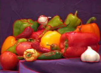
Fig (1) Segmentation for ValScale=300

Fig (2) Segmentation for ValScale=200

For this image 200 is a better ValScale Value.

3.2 Stop

This parameter regulates the execution of the isoperimetric Algorithm. This parameter is the maximum iso perimetric ratio allowable above which the algorithm execution stops. The below figures give the results of the isoperimetric algorithm for two values of Stop.

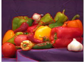
Fig (4) Segmentation for Stop=1e-4

These results show that 1e-5 is a better option for Stop parameter.

3.3 Connectivity Parameter

The pixels are compared with the neighboring pixels on the connectivity basis. We used two connectivity schemes which are 8-connectivity and 4-connectivity.

Fig(5) Segementation using 4-connectivity

Fig(6) Segmentation using 8-connectivity

8 is a better option 3.4 Cutoff

Fig (7) Segmentation for Cutoff =5

Fig (8) Segmentation for Cutoff =1000

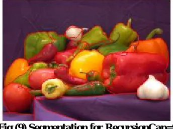
3.5 Recursion Cap

This parameter specifies the number of recursions that can take place for the partitioning algorithm on a particular segment and if exceeds considers the next partition for partitioning. It should be chosen such that over segmentation can be avoided. Practically in order to reduce the segmentation time it should be as less as possible.

Fig (9) Segmentation for RecursionCap=9

III. COMPARATIVE ANALYSIS

4.1) PSNR 4.2) RI

4.1. PSNR (Peak Signal to Noise Ratio)

Peak Signal-to-Noise Ratio, often abbreviated PSNR, is an engineering term for the ratio between the maximum possible power of signal and the power of corrupting noise that affects the fidelity of its representation. Because many signals have a very wide dynamic range, PSNR is usually expressed in terms of the logarithmic decibel scale.

PSNR is most commonly used to measure the quality of reconstruction of lossy compression codec’s (e.g., for image compression). The signal in this case is the original data, and the noise is the error introduced by compression. When comparing compression codec’s, PSNR is an approximation to human perception of reconstruction quality. Although a higher PSNR generally indicates that the reconstruction is of higher quality, in some cases it may not. One has to be extremely careful with the range of validity of this metric; it is only conclusively valid when it is used to compare results from the same codec (or codec type) and same content.

PSNR is most easily defined via the mean squared error (MSE). Given a noise-free m×n monochrome image I and its noisy approximation K, MSE is defined as:

1 1 2 0 0

1

[ ( , )

( , )]

m n i j

MSE

I i j

K i j

mn

 

 



_{ }



---(Eq. No.4.1) The PSNR is defined as

2

10

10. log (

MAX

I

)

PSNR

MSE



_{----(Eq. No.4.2)}

10

20.log (

MAX

I

)

MSE



10 10

20.log (

MAX

_I

) 10.log (

MSE

)





---(Eq. No. 4.3)

Here, MAXI is the maximum possible pixel value of the image. When the pixels are represented using 8 bits per sample,

this is 255. More generally, when samples are represented using linear PCM with B bits per sample, MAXI is 2B−1.

For color images with three RGB values per pixel, the definition of PSNR is the same except the MSE is the sum over all squared value differences divided by image size and by three. Alternately, for color images the image is converted to a different color space and PSNR is reported against each channel of that color space, e.g., YCbCr or HSL.

Typical values for the PSNR in lossy image and video compression are between 10 and 20 dB, where higher is better. In the absence of noise, the two images I and K are identical, and thus the MSE is zero. In this case the PSNR is undefined.

4.2. RI (Rand Index)

Image segmentation can be viewed as a special case of the general problem of clustering, as image segments are clusters of image pixels. Long ago, Rand proposed an index of similarity between two clustering’s. Recently it has been proposed that the Rand index be applied to image segmentations. Define a segmentation S as an assignment of a

segment label Si to each pixel ‘i’. The indicator function



( , )

s s

i j is 1 if pixels i and j belong to the same segment

(si=sj) and 0 otherwise. Given two segmentations S &

S



of an image with N pixels, define the function which is the fraction of image pixel pairs on which the two segmentations disagree.

1

1 ( , ) ( ) | ( , ) ( , ) | 2 i j i j i j N

RI S S  s s s s



  

_

    

---(Eq. No. 4.4) We will refer to the function

1



RI S S

( , )



as the Rand index, although strictly speaking the Rand index is

RI S S

( , )



similarity, but we will often apply that term to a measure of dissimilarity. In out statics the Rand index is applied to

compare the output

S



of a segmentation algorithm with a ground truth segmentation S, and will serve as an objective function for learning. A single wrongly classified edge of the affinity graph leads to an incorrect merger of two segments, causing many pairs of image pixels to be wrongly assigned to the same segment. The Rand index incurs penalties when pixels pairs that must not be connected are connected or vice versa. This corresponds to locations where the two matrices disagree. An erroneous merger of two ground truth segments incurs a penalty proportional to the product of the sizes of the two segments. Split errors are similarly penalized.

Hence RI is the measure of similarity between the two data images i.e. Accuracy, this index has a value in between 0 to 1. Higher value is better.

4.3 Comparative Analysis with Berkley’s output Image [14]

For comparative analysis we have taken the set of images from Berkeley’s Data base as a reference to compare with our project output. We have calculated the comparative parameters i.e. PSNR and RI.

Table: 4.1: Comparison Sheet

Input Image

Berkeley Segmentatio

n

Isoperimetri c Segmentatio

n

Analysi s

Ri- 0.9781 psnr-16.1409 Ri- 0.9751 psnr-14.1399

Ri- 0.9857 psnr-18.6742

Ri- 0.9883 psnr-18.5041 Ri- 0.9815 psnr-19.3250

IV. CONCLUSION

V. FUTURE SCOPE OF STUDY

We have presented a new algorithm for graph partitioning that attempts to find sets with a low isoperimetric ratio. Our algorithm was then applied to the problems of data point clustering and image segmentation.

These initial findings are encouraging. Since the graph representation is not tied to any notion of dimension, the algorithm applies equally to graph-based problems in N-dimensions as it does to problems in two dimensions. Suggestions for future work are applications to segmentation in space-variant architectures, supervised or unsupervised learning, 3-dimensional segmentation, and the segmentation/clustering of other areas that can be naturally modeled with graphs.

REFERENCES

[1]Leo Grady, “Isoperimetric Graph Partitioning For Data Clustering” IEEE TRANSACTIONS ON PATTERN ANALYSIS AND MACHINE INTELLIGENCE, VOL. XX, NO. Y, MONTH 2004

[2]Konstantinos D. Koutroumbas,” Piecewise Linear Curve Approximation Using Graph Theory And Geometrical Concepts”, IEEE TRANSACTIONS ON IMAGE PROCESSING, VOL. 21, NO. 9, SEPTEMBER 2012

[3]Mohamed Ben Salah, “Multiregion Image Segmentation By Parametric Kernel Graph Cuts”, IEEE TRANSACTIONS ON IMAGE PROCESSING, VOL. 20, NO. 2, FEBRUARY 2011

[4]R. Unnikrishnan, M. Hebert, “Measures Of Similarity”, Ieeeworkshop On Computer Vision Pplications, 2005, Pp. 394–400

[5]Y. Boy Kov, O. Veksler, And R. Zabih, “Fast Approximate Energy Minimization Via Graph Cuts,” IEEE Transactions On PAMI, 23 (11): 1222-1239, November 2004

[6]Yuri. Boykov And Vladimir Kolmogorov, “An Experiment Comparison Of Min-Cut / Max- Flow Algorithms For Energy Minimization In Vision”, IEEE Transactions On PAMI, 26 (9): 1124-1137, September 2004

[7]Vladimir Kolmogorov And Ramin Zabih, “What Energy Functions Can Be Minimized Via Graph Cuts?”,Ieeetransactions On PAMI, 26 (2): 147-159, February 2004

[8]D. Comaniciu, P. Meer, “Mean Shift: A Robust Approach Toward Feature Space Analysis”, IEEE Trans. On Pattern Analysis And Machine Intelligence, 2002, 24, Pp. 603-619

[9]J. Shi, J. Malik, “Normalized Cuts And Image Segmentation”, IEEE Transactions On Pattern Analysis And Machine Learning, 2000, Pp. 888-905.