ANALYSIS OF IMPORT DEMAND ELASTICITIES FOR KENYA: 1970 to
2013
PENINA WAITHIRA KAMAU
A RESEARCH PROJECT SUMBITTED TO THE SCHOOL OF
ECONOMICS IN PARTIAL FULFILLMENT OF THE RE~UIREMENTS
FOR THE AWARD OF THE DEGREE OF MASTER OF ECONOMICS
(FINANCE) OF KENYATTA UNIVERSITY
DECLARATION
This project is my original work and has not been presented for award of a degree in any other University.
Signature ~ . Date
2A\J9..\.2...9.\~
Penina Waithira Kamau (B.A. KU) Reg. No. KI02/PTICTY/214901201O.
This project has been submitted for examination with our approval as University supervisors.
Signature
~
.
Date
J
t
l(
f
f??.r.~
.
.
.
Prof. Nelson Wawire
Department of Applied Economic School of Economics Kenyatta University.
Signature
/
..
.
JIf
.
~~~~
.
~~
Date\i.l~~.f.~~
.
Dr. Steve Makori
DEDICATION
This research work is dedicated to Thomas Kamau my father, Eunice Nyawira my
mother, John Peter Muriuki my uncle and my lovely husband Fredrick Kinyua for
ACKNOWLODGEMENTS
I appreciate the handy work done by my supervisor Prof. Nelson Wawire and for
meticulously taking me through the research work. I'm sincerely grateful to Dr.
Steve Makori for providing me with guidance. To my family, I sincerely
acknowledge your continued moral and financial support in my academics.
Much appreciation goes to the Maker for answering my prayers and granting me
ABSTRACT
There was continued increase in imports volume and shrinking of exports. Due to government preoccupation with mobilizing external financial assistance, debt increased tremendously. The problem of growing population in Kenya, heavy importing and borrowing has led to current account deficit. Information on import demand elasticities was key to informing the tax policies that were to guide the taxation of imports and deciding optimal imports. The specific objective of the study were to estimate price elasticity of demand for imports, income elasticity of demand for imports and foreign exchange reserve elasticity of demand for imports The study analyzed the import demand elasticities using time series data from 1970 to 2013. Secondary data was used in the study. Data was collected from Central Bank of Kenya and Kenya National Bureau of Statistics documents. A multiplicative import demand function was estimated from which import elasticities were determined. The results show that income, relative price and foreign exchange reserve affect imports value. Long run elasticities were estimated and the coefficients of the variables were statistically significant expect for relative price. All the long run elasticities were found to be inelastic. Value of imports, relative price, income and foreign exchange reserve were co integrated in long run. The Kenya Revenue Authority can increase revenue collection from import duties. This was because import income elasticity for Kenya in long run was inelastic implying that imports responds to income is less than proportional. Export promotion policies should be encouraged as they increase foreign exchange reserves. This is because the results show that import demand respond to foreign exchange reserve. Borrowing efforts should be discouraged given that foreign exchange reserves elasticity was inelastic. This would improve balance of payments due to reduction in debts. Government can utilize imports of the previous period to forecast levels of tax revenue and also determine import behavior. This was because the lagged value of imports highly influences the demand of imports in Kenya.
TABLE OF CONTENTS
TITLE i
DECLARATION ii
DEDICA TION .iii
ACKNOWLODGEMENTS iv
ABSTRACT v
TABLE OF CONTENTS vi
LIST OF TABLES viii
LIST OF FIGURES ix
ABBREVIATION AND ACRONyMS x
OPERATIONAL DEFINITION OF TERMS xii
CHAPTER ONE: INTRODUCTION 1
1.1 Background 1
1.2 The statement of the problem 8
1.3 Research questions 9
1.4 Objectives ofthe study 10
1.5Significance of study 10
1.6Scope and limitation of the study 11
1.7 The organization of the study 11
CHAPTER TWO: LITERATURE REVIEW 12
2.1 Introduction 12
2.2 Theoretical literature 12
2.2.1 Mercantilism 12
2.2.2 The Neoclassical Trade Theory 14
2.2.3 The New Trade Theory 15
2.3 Empirical Literature 16
2.4Over view of the literature review 21
CHAPTER THREE: METHODOLOGy .23
3.1 Introduction 23
3.2 Research design 23
3.3 Theoretical framework 23
3.4 Model specification 25
3.6 Data type and sources 26
3.7 Stationarity 26
3.8 Correlation analysis 27
3.9 Cointegration 27
3.10 Data analysis 28
CHAPTER FOUR: EMPIRICAL FINDINGS 29
4.1 Introduction 29
4.2 Descriptive statistic and normality test 29
4.3 Stationarity analysis results 30
4.4 Correlation analysis results 32
4.5 Cointegration test results 33
4.6 Diagnostic and stability test results 34
4.7 Regression analysis results 37
4.8 Price elasticity of demand for imports 38
4.9 Income price elasticity of demand for imports 39
4.10 Foreign exchange reserve elasticity of demand for imports 40
CHAPTER FIVE: SUMMARY, CONCLUSION AND POLICY IMPLICATION .41
5.1 Introduction 41
5.2 Summary of the study 41
5.3 Conclusion 42
5.4Policy Implications 42
5.5Areas for further research .43
LIST OF TABLES
Table 3.1 Definition and Measurement of Variables 18
Table 4.1 Descriptive Statistic and Normality Test.. 21
Table 4.2 Stationarity Test Results 22
Table 4.3 Correlation Analysis Results 23
Table 4.4 Cointegration Test Results .24
Table 4.5 Diagnostic Test Results 26
LIST OF FIGURES
Figure 1.1: Kenya's of Balance of Payments 2
Figure 1.2:Kenya's value ofImports and GDP .2
Figure 1.3: Kenya's Current Account Deficit. .4
ABBREVIATIONS AND ACRONYMS
ADF Augmented Dickey Fuller
ARDL Autoregressive Distributed Lag
BOP Balance of Payment
CBK Central Bank of Kenya
CPI Consumer Price Index
ECM Error Correction Model
FDI Foreign Direct Investment
GDP Gross Domestic Product
GNP Gross National Product
IMF International Monetary Fund
KNBS Kenya National Bureau of Statistics
OECD Organization for Economic Cooperation and Development
OLS Ordinary Least Square
SNA System of National Accounts
SSA Sub-Saharan Africa
VECMVector Error Correction Model
OPERA TIONAL DEFINITION OF TERMS
Import:
Import income elasticity:
Import price elasticity:
Annual flow of goods and services from other countries in
the world to Kenya
percentage change in the quantity demanded of
imports due to a percentage change in income
(proxied by real GDP)
percentage change in the quantity demanded of
imports due to a percentage change in price of
imports (proxied by relative price)
Foreign exchange reserve elasticity: percentage change in the quantity demanded
of imports due to a percentage change in foreign
exchange reserve
Gross Domestic Product: The total market value of all final goods and services
produced in a country in a given year.
Exchange rate: Units of local currency per US dollar, adjusted for differential rates of
CHAPTER ONE
INTRODUCTION
1.1 Background
Since 1980 Kenya has been faced with fluctuations in Gross Domestic Product growth rate, balance of payment deficit and inflation rate. There was a 9.3 percent rise in fiscal deficit in 1981 (Republic of Kenya, 1984). The current account deficit also reached 11 percent of GDP in 1981. The inflation rate measured by CPI increased to an average of 18 percent in 1983 (Republic of Kenya, 1984).
In
1990, International Monetary Fund (IMF) pushed the government to adopt anexcessively demand management policy (Mwase, 1990). At the same period the economy fell into severe recession.
In
2000, the IMF and World Bank offered loans to the country to prevent a severe economic crisis with GDP growth falling to 0.2 percent (Republic of Kenya, 1990). Before, liberalization regime, the World Bank and IMF were routinely forcing developing countries to devalue their domestic currencies as one of the measures of economic recovery (Mwase, 1990). These measures were undertaken without assessing whether or not conditions for successful devaluation existed in these countries.In
1971, Kenya for example, made a decision to follow the U.S Dollar devaluation40000 20000
._---_._._---
._---":"::!
c
g
~ -20000 -HS-~--1!H!l-!S--l!HlHlH .5
E -40000
" E
E -60000
'0 ·80000"
-.~--11
I
ffi -100000 )ii -120000 [I
-140000-"---- ---
---Timein Years
-Balance of Paymentsin MillionKsh
Source: Republic of Kenya, Economic Surveys (various issues)
Figure 1.1: Kenya's of Balance of Payments
Balance of payments deteriorated and in 1994 it stood at ksh 5300 million. This
was contributed by weakening of capital account due to decline in official capital
inflows and increase in capital outflows (Republic of Kenya, 1995). The overall
balance deteriorated further in 1999 to a surplus of ksh 4240 million due to decline
in performance of capital and financial account (Republic of Kenya, 2000). It
further deteriorated in 2013 to a surplus of ksh 73922 million. The continuous
growth of imports volume has led to widening gap of balance of payments (Africa
Imports and GDP increased as depicted by the figure that follows.
[email protected] -- --.---.--.-.--- ..--.- ------.--.-------.---J. -~3000000+-·--··· - --- Jr···
~ ~
-~2500000+-.--- .. [
.5
";2~Or_---~--
---~
]
.~1500000 I - --
---E I
.g I
~ I
&1000000,...- -...--- ..---.-.. --..-.-.---. -... -.-
-500000 -t-__....
I
o· , I , , ,--,
~~~~~~#~~~~~~~~$
~
~~~~~~~##~#~#~#~~~~
--l
I
I
I
-KenyaGDP
I
-Imports I
I
I
I
I Source: Republic of Kenya, Economic Surveys (various issues)
Figure 1.2: Kenya's value ofImports and GDP
The figure shows that there was a positive relationship between the value of imports and GDP. Imports contribute to the GDP as expenditure. This means that as expenditure on imports of goods and services increases, the GDP increases. In year 2013 both GDP and imports recorded the highest value of ksh 3,797,987 million and ksh 1,413,316 million respectively (Republic of Kenya, 2014). Due to increase in volume of imports, some local industry has closed and this has led to
massive unemployment of youths. Liberalization of the Kenyan Economy in 1993 meant great competition from imported clothing (Republic of Kenya, 1995).There was increased importation of textiles especially second hand,
"mitumba
"
,
financial difficulties experienced by the local producers led to closure of textile firms such as KICOMI, Allied Industries Limited and Heritage Woolen Mills.
Robert (2005) explained that a current account deficit implies an excess of imports over exports of goods, services, investment income and unilateral transfers. This leads to an increase in net foreign claims upon the importing nation. The importing nation becomes a net demander of funds from abroad, the demand being met through borrowing from other nations or liquidating foreign assets. The result is a worsening of the importing nation's net foreign investment position. The current account balance thus represents the bottom line on a nation's income statement. If it is positive, the nation is spending less than its total income and accumulating asset claims on the rest of the world. If it is negative, domestic expenditure
exceeds income and the nation borrows from the rest of the world.
According to Osoro (2012), increase in the value of imports in most developing economies is largely due to the increase in prices of Petroleum; oil lubricants,
fertilizers, and food grains.
The goals of Vision 2030 is to improve manufacturing by reducing imports in key local industries, growing market share in regional market and attracting atleast 10 large strategic investors in key agro-processing industries. Kenya is also aiming at
services, the external current account deficit widened gradually to 6.7 per cent of
GDP in 2009, reflecting the strong increase in imports associated with increased
foreign direct investment and higher disbursement of long term capital for
investment spending. However, net capital inflows were expected to be more than
offset the deficit in the current account thereby facilitating an overall balance of
payments surplus. This was in turn to help the government further build up
adequate foreign reserves to the equivalent of 4.7 months of import cover by 2012
which was a way to cushion the economy from external vulnerabilities including
high oil prices and drought effects. This was an equivalent of 6 months import
cover using the previous years import bill (Republic of Kenya, 2008).
The year 1997 was a turning point in Kenya's trade balance when it recorded a
deficit of US$ 885.9 million, thereafter there was a huge increase in trade deficit
due to slow growth of export and fast growth in imports (Osoro, 2012). Kenya has
reported a worrisome, deficit over decades, which means that large amounts of the
Kenyan shilling leave the country. These outflows have driven the value of the
Kenyan currency down, making it more costly to purchase imports. Policy reforms
have had an impact on the balance of payment which affects the performance of
the economy. Resumption of economic growth led to increase in imports than
exports, contributed to further deterioration of Kenya's trade deficit in 1995 and
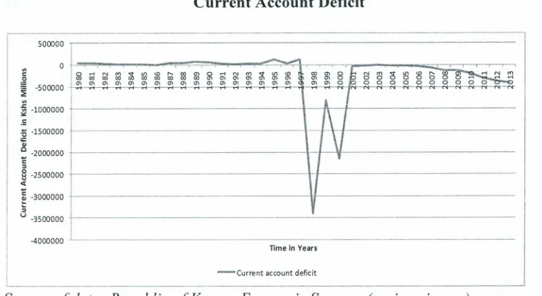
Current Account Deficit
500000
-1000000t---+---J\-t---
---1500000i-···-··---····-···-·-··-···-···---·--·----·l
-2000000 -.- ..•.•.•
·2500000
-3000000+---11
---3500000t--- ---
---4000000 ._---_..
_---TimeinYears
I -Current accountdeficit
~.---Source of data: Republic of Kenya, Economic Surveys (various issues)
Figure 1.3: Kenya's Current Account Deficit
The current account worsened. Earnings from merchandise exports declined while
import bill increased in 2013. The trade deficit expanded as a result of marked
increase in value of imports and a decrease in value of exports (Republic of
Kenya, 2014).
With the new government in 2003 the economy started recovering and surplus in
current account was recorded. From 2004 Kenya has run a current account deficit
since then and in 2011 it recorded a deficit of KShs. 359,463 million (Osoro,
2012). This was contributed by higher oil prices which led to inflation increase.
Exports stagnated and earnings from the exports were not enough to cover oil
importation.
Imports are dominated by industrial supplies with a share of 36 percent of total
total imports while food and beverages constituted an average of 8 percent. Kenya is also having heavy imports of crude oil. Manufactured goods account for most of the imports from European Union, the United States and Japan. Tariffs have been the main trade policy instrument, however since Kenya became a member of World Trade Organization overall protection has been reduced (Manitra, 2011).
Exchange rate policy plays a key role in determining a country's international competitiveness. If the real exchange rate depreciates, a country's exports become more attractive to the rest of the world, while imports become relatively more expensive, thus favoring domestic production.
Foreign aid represents an important source of finance for many countries in sub-Saharan Africa (SSA), where it supplements low savings, narrow export earnings and thin tax bases. Most of African countries have been receiving foreign aid from the United States responds to African humanitarian crises. Organizations such as World Bank and IMF have been lending funds. Kenyan government has been
seeking foreign assistance too.
With regard to international trade, foreign currency IS often a necessary
requirement to finance imports of goods and services. In this sense, foreign reserves play the role of an international liquidity constraint and any increase in reserves should thus have a positive impact on import demand (Arize and Osang, 2007).
finance declined in 1980s due to sharp increases in interest rates (Mullei and
Scaperlanda, 1986 and Khan and Montles, 1987). The external debt service
payments have cut into export earnings thereby, exerting greater pressure on
Kenya's ability to import essential goods.
Information on elasticities is important in coming up with trade policies that are
friendly. For developing countries in particular, estimates of secular elasticities are
of practical importance for examining the effects of import price, income, foreign
exchange reserve and foreign asset on demand for imports as well as for analyzing
the welfare implications of the cross-sectional structure of trade. For instance,
Grossman and Helpman (1994), in the endogenous trade policy context, predict
that the industries with high import demand elasticities are given less protection
since the deadweight loss from trade diversion in those industries is higher. This
sort of welfare analysis depends on the information about these elasticities.
1.2 The Statement of the Problem
Imports help in increasing the utility of the consumer through raising the level and
variety of goods and services consumed. Import demand elasticities are important
for examining the effects of relative price, income and foreign exchange reserve
on the value of imports. For foreign trade policy implementation, it is important to
determine import and export demand elasticities. Elasticities are also essential in
making policy decisions on optimal trade volume and making decisions on import
In Kenya, appetite for imported goods is raismg and market for exports is
shrinking. There has been a bulky import of machinery and equipment for
investment and consumable goods. In the local markets, the imported goods are
cheaper compared to the locally processed goods (Manitra, 2011). Kenya's
growing population places demand on imported goods and services. Therefore,
population growth, infrastructural improvement and manufacturing activities lead
to increased volume of imports. The government has to make prudent decisions
about the volume of imports as envisaged in Kenya's Vision 2030 (Republic of
Kenya, 2007). This can only be done if there is availability of information on
import demand elasticities.
Unavailability of import demand elasticities information is dangerous to the
economy and especially to policy makers. It means optimal import demand
decisions cannot to be determined. Foreign exchange reserves also determine
imports demands (Mwega, 1993).
The purpose of the study was to estimate an import demand function from which
import demand elasticities are to be derived.
1.3 Research Questions
1. What is the price elasticity of demand for imports?
11. What is the income elasticity of demand for imports?
111. What is the foreign exchange reserve elasticity of demand for imports?
1.4 Objectives of the Study
The general objective of the study was to estimate and analyze import demand
elasticities for Kenya.
The specific objectives were to estimate:
1. Price elasticity of demand for imports
11. Income elasticity of demand for imports
111. Foreign exchange reserve elasticity of demand for imports.
1.5 Significance of Study
To achieve efficient policy formulation, it is necessary for the policy makers such
as government and Central Bank to have knowledge of not only the signs, but also
the magnitude and stability of the response of the relevant variables that are
required for policy decision making. The derived estimates are to be used not only
as an analytical tool in decision making, but also as an instrument for economic
forecasting of demand for imports
The estimation results are to be used to assist the Kenya Revenue Authority and
the Treasury in forecasting the level of tax revenue from import sources, as
knowledge of the behaviour of imports will inform the behaviour of import tax
revenue. The study also provided a basis for the formulation of international trade
policy coordination in Kenya for both bilateral and multilateral trade relations, as
well as useful input for macroeconomic modelling of the Kenyan economy. The
1.6 Scope and limitation of the Study
The study focused on estimating and analyzing import demand elasticities for
Kenya. The study covered a period of forty four years from 1970 to 2013.
Data on foreign exchange reserve and foreign asset were not readily available for
periods before 1970 hence the period of the study was 1970 to 2013.
1.7 The organization of the study
The study is organized into five chapters. Chapter one contains introduction,
statement of the problem, research questions, objectives of the study, significance
of the study, scope and limitation of the study. Chapter two presents literature
review both theoretical and empirical and overview of the literature review.
Chapter three focuses on methodology which includes the research design,
theoretical framework, model specification, definition and measurement of
variables, data type and sources and data analysis. Chapter four contains data
analysis and interpretation of the results. Chapter five focuses on summary,
CHAPTER TWO
LITERA TURE REVIEW
2.1 Introduction
This chapter contains theoretical literature which links the study with the existing
theories. It has empirical literature review which portrays linkage between
literature review and objectives of the study and research questions. It indicates
related work done by other researchers and the knowledge gap. Finally there is
overview of the literature in which the knowledge gap is identified.
2.2 Theoretical literature
The international trade literature suggests three major theories of the import
demand: The Mercantilism, the new trade theory (also known as the imperfect
competition theory of trade) (Hong, 1999) and the Neoclassical Trade Theory
2.2.1 Mercantilism
The view of mercantilism was to maximise net exports and it was the best route to
national prosperity. In Mercantilism the idea that the only true measure of a
country's wealth and success was the amount of gold that it had. If one country
had more gold than another, it was necessarily better off. This idea had important
consequences for economic policy. The best way of ensuring a country's
prosperity was to make few imports and many exports, thereby generating a net
inflow of foreign exchange and maximising the country's gold stocks (Robert,
It was the dominant economic doctrine for more than three centuries (16th - 18th),
mostly associated with the colonization era. It was often dubbed economic
nationalism where the efforts to boost exports were backed by a powerful state
protecting domestic monopolies (such as the British East India Company). It was a
way nation-states were competing with each other. The nation which had more
gold had more wealth and it could raise a stronger army, and thus be more
powerful. The role of colonies was crucial in this power struggle, as they were the
source of precious metals and raw materials, and on the other hand the recipients
of exported goods (Robert, 2005).
Mercantilism was characterized by a triangular trade system, where European
countries were exporting manufacturing goods and textiles to Africa and America,
America was sending raw materials to Europe, while Africa was sending slaves to
America. After all, during the period of mercantilist dominance, the living
standards of the population were still miserable, not much better than during the
hunter-gatherer times (Robert, 2005).
A big part of the mercantilist doctrine was protectionism. More precisely
protectionism of business interests against any forms of competition. Governments
applied many forms of different protectionist policies, from guild rules and taxes,
tariffs and quotas, prohibitions of imports to big state-run monopolies. It provided
capital to exporting industries and even prohibited exports of tools (technology)
and skilled labour that would allow foreigners to produce the same goods the
2.2.2 The Neoclassical Trade Theory
In the neoclassical trade theory of comparative advantage, as characterized by the
Heckscher-Ohlin framework extended from the classic Ricardian theory, the focus
is on how international trade, its volume and direction, is affected by world prices
and domestic prices , which in turn are explained by the differences in factor
endowments between countries. The effects of changes in income on trade is not
the concern the level of employment is assumed to be fixed and output is assumed
to be always on a given production frontier (Ethier, 1983).
While the neoclassic import demand function which estimate both prices and
income elasticities is based on the assumed neoclassical microeconomic consumer
behavior and general equilibrium framework, as distinguished from the
neoclassical comparative advantage analysis, relative prices are assumed to be
rigid and employment is variable (Dixit and Norman, 1980). Further, international
capital movements are not assumed away and they are passively adjusted as
required by the trade balance. So, this theory focuses on the relationship between
income and import demand at the aggregate level and in the short term. The
relationship can be defined by a few ratios, such as the average propensity to
import, the marginal propensity to import which describes responsiveness of
import volumes and the income elasticity of imports competition theory of trade,
the latest school in trade theory, and the intra-industry trade, which is not
explained well by the theory of comparative advantage. The analytical framework
of this theory depends on specific assumptions about the market structure that give
rise to increasing returns. Details can be found in (Dixit and Norman, 1980),
(Helpman, 1981), (Grossman, 1992) and (Krugman, 1987). By applying the
general equilibrium framework to the global economy, the analytical form of the
neoclassical import demand function is defined as follows (Dixit and Norman,
1980).
M (P)=D(P ,E(P,u))- S(P) 2.1
Where M is the real demand for imports, P is the relative price of imports both
import price index and consumer price index. D is the total demand for importable
goods, derived from the optimal consumer assumption, E is expenditure at the
given relative price P and the given utility level u, S is the domestic supply of
importable goods. The elasticity form is as follows:
e=c-s-m 2.2
Where e is the elasticity of import demand, c is the demand substitution elasticity,
s is the supply substitution elasticity and m is the marginal propensity to import.
By the same token, one can also define the import price elasticity of the foreign
country as e*. The summation of the absolute value of both e and e* plays an
important role in international trade policy analyses. For example,
1
e1+ 1
e*l> 1,which is the Marshall-Lerner condition, defines a condition for the stability of
international trade equilibrium (Dixit and Norman, 1980)
2.2.3 The New Trade Theory
The new trade theory explains the effects of economies of scales, product
differentiation, and monopolistic competition on international trade. There are
market effects on international trade: Marshallian, Chamberlinian, and Cournot
approaches. The Marshallian approach assumes constant returns at the firms level
but increasing returns at the industry level, the Chamberlinian approach on the
other hand assumes that an industry consists of many monopolistic firms and new
firms are able to enter the market and differentiate their products from existing
firms so that any monopoly profit at the industry level can be eliminated (Dixit and
Norman, 1980). The Cournot approach assumes a market with only a few
imperfectly competitive firms where each takes each other's outputs as given.
With anyone of these three market structures, an opening of international trade
will lead to a larger market size, decreasing costs and more output and trade the
volume of imports will increase (Dixit and Norman, 1980). Hence the new trade
theory suggests a new link between trade and income as the role of income in
determining imports goes beyond that defined in the neoclassic import demand
functions, where income only affects purchasing power.
2.3 Empirical Literature
Moazzami and Wong (1988) estimated aggregate import demand function for
China. The study used partial adjustment model with 17 annual observations from
1970 to 1986. Relative price and disaggregated GDP which included: exports, real
investment, real private and public consumption and real disposable income.
Autoregressive Distributed Lag Model was used to derive long run and short run
coefficients. The study results showed that the relative price had negative effects
and macroeconomic variables had positive effects to trade volume. Domestic
and aggregate exports appear to be important determinants of the relevant types of import demand in the long run and short run. The long-run elasticities are found to
be elastic. The current study will utilize aggregated real GDP rather than dissagregated GDP. One key conclusion is that high dependency on investment to promote economic growth may lead to consequent deterioration on balance of
trade. This is what is happening in Kenya (Republic of Kenya, 2013).
Mwega (1993) estimated demand elasticities for aggregate imports and component in Kenya over 1964 -91. An error correction model was utilized to estimate elasticities. Mwega (1993) showed that shortrun relative price and real aggregate import demand elasticities were weakly significant. Mwega (1993) used an error correction model and CHOW test to estimate the elasticities for aggregate import and its components, and testing for stability of import demand during trade liberalization in Kenya for the period 1964-1991. Conversely, aggregate imports
were strongly responsive to lagged foreign assets and foreign receipts. The CHOW test revealed the stability of the function.
elasticities, the significant positive sign was estimated and they were also
significant. The study will be relevant to current study as foreign aid and foreign
exchange reserve were present in Bangladesh study.
Sinha (1997) estimated an aggregate import demand function for Thailand using
annual data for the period, 1953-90. The study had used the traditional variables
relative price and real GDP. The study had utilized the current time series analysis,
cointegration approach, Johansen Jeselius. The study showed that aggregate
import demand for Thailand was price inelastic, cross price inelastic (with respect
to domestic price) and income inelastic in the short-run. In the long-run, aggregate
import demand was still price inelastic and cross price inelastic. However,
aggregate import demand was highly income elastic in the long run. The study was
relevant as the country experiences current account deficit and had high
importation of capital goods and oils same as Kenya.
Egwaikhide (1999) estimated import demand usmg an error correction
specification for an import demand model for Nigeria and indicated that foreign
exchange earnings, relative prices and real income all significantly determined the
behavior of total imports in the reference period. The study aim was to determine
the effects of various trade reforms particularly the liberalization policy since the
mid-1980s on the import demand behavior of Nigeria. Findings also show that
short-run import decisions are determined by the dynamics of foreign exchange,
which are tied to the long-run effect through the feedback mechanism. The results
of the disaggregated imports reveal the importance of foreign exchange. The
and had similar Structural Adjustment Programme which was inspired by IMF and
World Bank such as in Kenya.
Kotan and Saygili (1999) estimated an import demand function for Turkey. The
main aim of the study was to assess Turkish import developments of domestic
income, exchange rate and foreign exchange movements. This study incorporated
two different model specifications to estimate an import demand function for
Turkey. The estimation performance of the two models was compared and
contrasted for the period 1987Q 1-1999Q 1 by using quarterly data. The
significance of variables that affect import demand were individually and jointly
tested. Also, the short run elasticities of the two models are compared. The first
model estimated imports using Engle Granger found that in the long run, in?ome
level, nominal depreciation rate, inflation rate and international reserves
significantly affect imports. The second approach modelled import demand using
the Bernanke-Sims structural VAR method. The findings indicated that anticipated
changes in the real depreciation rate and unanticipated changes in the income
growth and real depreciation rate. The Turkey study assisted in comparing the
results of Engle Granger approach, Bernanke-Sims structural VAR method and
Johansen approach. Engle Granger approach this approach has its own
shortcoming compared Johansen Jeselius. In the study for Turkey Inflation rate
was determined in the model. In the current study relative price which is aratio of
Previous studies done low import price elasticities were portrayed using ordinary
least square method or fixed effect method. Industries producing homogeneous products price elasticities were higher than in those producing differentiated ones.
In long run average price elasticities were higher than one and close to zero in short run. A study in Malysia estimated the long-term relationship between import demand, and its determinants, namely income and relative prices, a robust estimation method known as the Unrestricted Error Correction Model Bounds Test Analysis was used (Cheong and Nair, 2002). The results showed that import volume, income and relative prices were cointegrated. The estimated long run elasticities of import demand with respect to income and relative prices were1.5 and -1.3 respectively. This implied that monetary, fiscal and exchange rate policies could be used as instruments to maintain favorable trade balance.
Musyoka (2010) estimated compensated and uncompensated elasticities. The study used import demand function for cereals. Three estimators were utilized in estimation of elasticities which were Ordinary Least Square, Instrument Variable and Seemingly Unrelated Regression Equations. The conclusion was that uncompensated elasticities were bigger in magnitude than the compensated elasticities. The study recommended removal of the tariff rate and alternative ways of improving domestic wheat production rather than import restrictions. This study
was conducted in Kenya and it relates to current study as it estimated elasticities of
cereal imports.
Harvey and Sedegah (2011) studied import demand in Ghana, its structure,
imports volume, Openness Trade Index, and foreign assets have been used in the
study. Co integration and error correction models had been used to estimate the
model. Aggregated and disaggregated imports demand functions are estimated.
The results of the study indicated that domestic income, foreign exchange reserves
and trade liberalization played a significant role both in the long run and short run
imports demand levels in Ghana. There was also parameter stability in import
demand function in the period under the study. The aim of the trade policies
authority was to reduce imports to correct balance of payment deficits in the long
run. The current study uses similar variables used by Harvey and Sedegah, 2011.
2.4 Over view of the literature review.
The three theories that is the neoclassic trade theory, the Mercantilism, and the
new trade theory assume that in a market economy, import demand Can be fully
modeled by income and relative prices. All other factors can be theoretically
sub-modeled within these two factors (Tang, 2003).
In most studies the traditional variables are used that is real GDP and relative
prices except for Turkey study. Other variables such as Foreign Aid, Foreign
exchange reserves, international reserves, nominal depreciation rate have been
included in the various studies under review. Imports volume has been widely
used as the dependent variable.
In various study time analysis have used. Cointegration approaches such as Engle
Granger, Johansen approach have been used to test co integration among the
Many studies have been conducted by the researchers and the results show that in
short run price elasticity is inelastic in long run price elasticities are elastic.
Various studies have shown that Real GDP has positive effect to imports volume
and relative price has negative effects to trade volume. In developing countries
under review foreign exchange is a major determinant of imports. Also foreign aid
variable is a major determinant of trade volumes. Parameters in most studies are
stable in period under the studies.
In the current studies various elasticities of imports were determined which
include income, price and foreign exchange reserve. Most studies have determined
CHAPTER THREE
METHODOLOGY
3.1 Introduction
The chapter contains research design, theoretical framework, definitions and
measurement of variables, estimating model, data types, source and data analysis.
3.2 Research design
The research design which was adopted in the study was descriptive. The study
specifically adopted a non- experimental time series research design. Time series
data was collected for the period 1970-2013. The data was subjected to time series
properties tests. Correlation analysis was also done to determine the relationship
between independent variables. Cointegration analysis was done as it allowed non
stationary data to be used so that spurious results are avoided. Ordinary Least
Squares estimation was done to determine the import demand elasticities.
3.3 Theoretical Framework
Neoclassical theory of comparative advantage characterized by the
Heckscher-Ohlin theory was adopted. It explains how international trade is affected by
volume of imports and relative prices due to difference in factor endowment
between the countries. Neoclassical import demand function was adopted to
estimate elasticities of import demand. It was based on neoclassical
microeconomic consumer behavior. Microeconomic consumer behavior was used
to identify the relevant variables of the import demand, function as derived from
Assuming maximization of utility of two goods XI and X2• Importer will to
maximize the following general utility function.
Max u
=
(XI X2) .•.•....•..••.•..•...•. 3.1Subject to
PIXI
+
P2X2=
Y 3.2U
=
utilityXI =imports
X2 = other goods
PI
=
priceP2
=
price for other goodsFrom equation 3.1 and 3.2 lagrangrian composite equation is;
From equation 3.3 the first order condition for utility maximization is as follows:
aL
l
ax
l=
X2- API=
0 3.4aL
l
ax
2=
XI- AP2=
0 3.5aL
i
a
A=
PIXI+
P2X2 - Y=
0 3.6From the first order conditions, import demand function is derived
However, import does not only depend on price and income but also on other factors. The other factor include: foreign exchange reserve (Dutta and Ahmed,
1997). The following equation was therefore estimated:
X, = f(Y,P,FER) 3.8
P =Price
Y =Income
FER = Foreign Exchange Reserve
3.4 Model Specification.
To derive elasticities, it was appropriate to estimate a log-linear demand function of the following specification:
(M)t= value of import for year t (Y) t= real GDP foryear t
(RP)t= relative import prices for year t
(FER)t = current foreign exchange reserves inyear t
To linearize by taking the logarithm of the variables yield the following equation:
3.5 Definition and measurement of variables
Table 3.1 Definition and measurement of variables
Variable Definition Measurement
Value of Imports (M) Annual value of goods Value of imports
and services flow from measured in Ksh.
other countries III the
world to Kenya.
Real Gross Domestic This is a measure of Nominal GDP deflated by
Product (Y) economic output adjusted GDP deflator.
for price changes (is a
proxy for income)
Relative prices (RP) Ratio of import pnce Real relative price.
index and consumer price index
Foreign exchange reserve Foreign-exchange Foreign exchange reserve
(FER) reserves are assets held will be measured in Ksh.
by central banks and
monetary authorities
3.6 Data Type and Sources
Secondary data was collected for forty four years from 1970-2013. The data
collected from the period was annual. The GDP for Kenya was collected from
CBK annual reports while value of imports, foreign asset, foreign exchange
reserve, import price index and consumer price index was collected from KNBS
Economic Survey annual publications.
3.7 Stationarity
Time series data usually exhibit a non-stationary process and if OLS method is
applied directly the results would be spurious. Because of this a test for stationarity
was done. Unit root test on both dependent and independent variables in the model
was conducted to evaluate their time series characteristics. The test was to
The basic logic here was to avoid the problem of spurious regression. For this
purpose Agumented Dickey-Fuller (Dickey and Fuller, 1981) was employed to
determine stationarity.
i-l
~Yt
=
aYt-l +L~~Yt-i
+8 + 'Yt+Et for levels 3.11/II
i-I
~ ~Yt
=
aYt-l +L ~~
~
Yt-i +8 + 'Yt+Et for first difference 3.12/II
Where: Y is the variable whose stationarity is being examined, M is the number of
lags and trepresents time. If the null hypothesis is rejected then it means that the
time series data is stationary.
3.8 Correlation analysis
Correlation was done to determine the relationship between the regressors that
was, price, income and foreign exchange reserve. This was to help establish if
there was a problem of multicollinearity or not. If the independent variables are
strongly correlated one of them was removed to avoid biased estimated
parameters.
3.9 Co integration
Cointegration analysis allows non stationary data to be used so that SpurIOUS
results area avoided. It establishes whether there is a long-run causal relationship
between the dependent variable and the independent variables. The cointegration
analysis was carried out within the Johansen (1992) framework using the
because it offers the means to determine whether there IS more than one
cointegrating vector.
The Vector Autoregression (VAR) based cointegration test methodology by Johansen is described under a VAR of order p:
Yt=Ayc, + +ApYt-p+BZt+f.!t 3.13
Where Y, is a vector of non-stationary 1(1) variables Z,is a vector of deterministic variables and f.!tis a vector of other variables not in the model. This test is robust to any departure from normality since it gives room for normalization with respect to any variable in the model that becomes the depended variable. If the Maximum Eigen value test and trace test confirm presence of co integrating equation then there exists a long run relationship between the variables.
3.10 Data Analysis
The objectives of the study were attained by estimating a log linear import demand function as explained in section 3.1
o.
Specification of a log linear form waspreferable when estimating import demand function as the use of this form allowed the interpretation of the coefficients as elasticities
B
1 coefficient of InYtwas to measure income elasticity of demand for imports.
B2
coefficient of In RPt was to measure price elasticity of demand for imports. B3 coefficient of In FERtCHAPTER FOUR
EMPIRICAL FINDINGS
4.1 Introduction
This chapter deals with the presentation and interpretation of empirical findings of
the study. It focuses on descriptive statistics of each variable both dependent and
independent variables. It also contains stationarity test results, correlation analysis
results and cointegration results. The chapter also focuses on diagnostic test which
include serial correlation, heteroscedasticity and functional form test. Normality
test is also discussed in this chapter. Finally the chapter analyzes regression results
and every elasticities is analyzed.
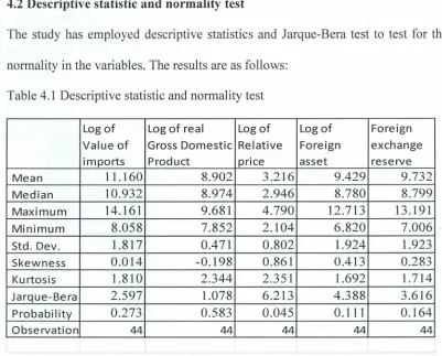
4.2 Descriptive statistic and normality test
The study has employed descriptive statistics and Jarque-Bera test to test for the
normality in the variables. The results are as follows:
Table 4.1 Descriptive statistic and normality test
Logof Log of real Log of Logof Foreign
Value of Gross Domestic Relative Foreign exchange
imports Product price asset reserve
Mean 11.160 8.902 3.216 9.429 9.732
Median 10.932 8.974 2.946 8.780 8.799
Maximum 14.161 9.681 4.790 12.713 13.191
Minimum 8.058 7.852 2.104 6.820 7.006
Std. Dev. 1.817 0.471 0.802 1.924 1.923
Skewness 0.014 -0.198 0.861 0.413 0.283
Kurtosis 1.810 2.344 2.351 1.692 1.714
Jarque-Bera 2.597 1.078 6.213 4.388 3.616
Probability 0.273 0.583 0.045 0.111 0.164
Observation 44 44 44 44 44
Where log means Natural Logarithm
Table 4.2 above reveals that the Jarque-Bera statistic after logarithmic
transformation of the variables is not significantly different from zero, thereby
implying that all the variables are normally distributed at 5% significance level
except log of relative price as the p value is 0.045 which was less than 0.05. The
other descriptive statistics for the variables are summarized in table where the
standard deviation for Log of Foreign asset is 1.923 suggesting that it was the most
volatile variable among the data set over the entire duration under observation
4.3 Stationarity analysis results
To perform a stationarity test on the individual time series, evaluation on each of
the variables for the presence of a unit root using the Augmented Dickey-Fuller
(Dickey and Fuller, 1981) test. The test is based on the regression for both level
and first difference. The following table shows results for unit root tests.
Table 4.2 ADF Unit Root test in Levels and First Difference
Variable Calculated value 5% Critical value Decision Table 4.2 stationarity analysis results
withtrend withtrend
and with and
withintercept intercept none intercept intercept none
LogM -0.228 -2.789 5.081 -2.932 -3.519 -1.949 Not- stationary
DLogM -6.325 -6.227 -2.586 -2.934 -3.522 -1.949 Stationary
LogY -0.943 -2.058 3.206 -2.932 -3.519 -1.949 N ot- stationary
DlogY -4.569 -4.501 -3.253 -2.934 -3.522 -1.949 Stationary
LogRP -1.919 -2.111 -1.945 -2.932 -3.516 -1.949 Not- stationary
DlogRP -5.564 -5.548 -4.953 -2.934 -3.522 -1.949 Stationary
Log FER 0.007 -2.812 2.675 -2.932 -3.519 -1.949 Not- stationary
DlogFER -6.672 -6.703 -5.101 -2.934 -3.522 -1.949 Stationary
LAGM 0.023 -2.645 5.233 -2.934 -3.522 -1.949 Not- stationary
Source: Own calculations
Log M- Natural Logarithm of value of imports
D Log M- Differenced Natural Logarithm of value of imports
Log Y- Natural Logarithm of real Gross Domestic Product
D Log Y- Differenced Natural Logarithm ofreal Gross Domestic Product
Log RP- Natural Logarithm of Relative Price
D Log RP- Differenced Natural Logarithm of Relative Price
Log FER- Natural Logarithm of Foreign Exchange Reserve
D FER- Differenced Natural Logarithm of Foreign Exchange Reserve
LAGM- Lagged value of imports
D LAGM- Differenced Lagged value of imports
The ADF test was employed both with intercept, with intercept and trend and
without intercept and trend. The decision criterion involved comparing the
computed tau values with the Mackinnon (1999) critical values for the rejection of
a hypothesis with a unit root. For tests at levels in table 4.2 the computed tau
statistics are greater than the MacKinnon critical tau values, and thus null
hypothesis was not rejected the null hypothesis that the time series data variables
are non-stationary at levels. On the other hand, the computed tau statistics are less
than the MacKinnon(1999) critical tau values at first difference and this means at
first difference all variables are stationary.
This test further confirms that all the variables are non-stationary in levels at 5%
significance level. The meaning of this is that, the time series data have a
a shock strikes and the distributions have no constant mean or variance. The non-stationary variables exhibit difference stationarity because they are integrated of order one [1(1)] implying that they should be differenced once to attain stationarity. After the confirming that the order of integration is the same, test for Co-integration followed.
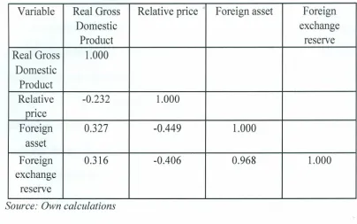
4.4 Correlation Analysis Results
Table 4.3 presents correlation coefficients for the variables
Table 4.3 Correlation Analysis Results
Variable Real Gross Relative price Foreign asset Foreign
Domestic exchange
Product reserve
Real Gross 1.000 Domestic
Product
Relative -0.232 1.000
pnce
Foreign 0.327 -0.449 1.000
asset
Foreign 0.316 -0.406 0.968 1.000
exchange reserve
Source: Own calculations
and Foreign asset.The procedure used to detect the presence and severity of
multicollinerity by Koutsoyiannis (1977) was applied. The procedure involves
regressing the dependent variable on each of the explanatory variables separately.
The results obtained from regression are assessed on the basis of priori and
statistical criteria. Regression which appeared to give the most plausible results
was adopted. Foreign asset was dropped for the purpose of this study. Then there
insertion of other additional variables and examine effects on individual
coefficient, standard error and overall R2. A new variable namely lagged imports
value was introduced which improved overall R2 and also Durbin Watson.
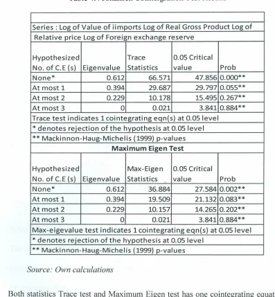
4.5 Cointegration Test Results
The time series variables exhibited a stochastic trend. So to investigate if there was
any long-run relationship was necessary. This study then employed the Johansen
cointegration test, which is to a greater extent more superior to the Engle and
Granger two step procedure. The Vector Autoregression (VAR) based
co integration test methodology by Johansen is described under a VAR of order p.
Basically the test also involved the Maximum Eigen test and the Trace statistics
which are employed in the analysis. The results are presented in the table that
Table 4.4 Johansen Cointergration Test Results
Series: Log of Value of iimports Log of Real Gross Product Log of
Relative price Log of Foreign exchange reserve
Hypothesized Trace 0.05 Critical
No. of C.E (s) Eigenvalue Statistics value Prob
None* 0.612 66.571 47.856 0.000**
At most 1 0.394 29.687 29.797 0.055**
At most 2 0.229 10.178 15.495 0.267**
At most 3 0 0.021 3.841 0.884**
Trace test indicates 1 cointegrating eqn(s) at 0.05 level
* denotes rejection of the hypothesis at 0.05 level
** Mackinnon-Haug-Michelis (1999) p-values
Maximum Eigen Test
Hypothesized Max-Eigen 0.05Critical
No. of C.E (s) Eigenvalue Statistics value Prob
None* 0.612 36.884 27.584 0.002**
At most 1 0.394 19.509 21.132 0.083**
At most 2 0.229 10.157 14.265 0.202**
At most 3 0 0.021 3.841 0.884**
Max-eigevalue test indicates 1 cointegrating eqn(s) at0.05 level
* denotes rejection of the hypothesis at 0.05level
** Mackinnon-Haug-Michelis (1999) p-values
Source: Own calculations
Both statistics Trace test and Maximum Eigen test has one co integrating equation
thereby implying that there exists aunique long-run relationship between the set of
variables. The results showed that import demand for Kenya is co integrated in the
longrun. The lag length was 4.
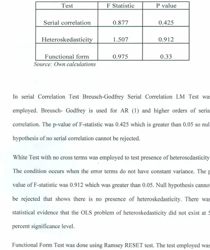
4.6 Diagnostic and Stability Test Results
The diagnostic test include serial correlation, heteroskedasticity and fuctional form
Table 4.5 Diagnostic Test Results
Test F Statistic P value
Serial correlation 0.877 0.425
Heteroskedasticity 1.507 0.912
Functional form 0.975 0.33
Source: Own calculations
In serial Correlation Test Breusch-Godfrey Serial Correlation LM Test was
employed. Breusch- Godfrey is used for AR (1) and higher orders of serial
correlation. The p-value of F-statistic was 0.425 which is greater than 0.05 so null
hypothesis of no serial correlation cannot be rejected.
White Test with no cross terms was employed to test presence ofheteroscdasticity.
The condition occurs when the error terms do not have constant variance. The p
value of F-statistic was 0.912 which was greater than 0.05. Null hypothesis cannot
be rejected that shows there is no presence of heteroskedasticity. There was
statistical evidence that the OLS problem of heteroskedasticity did not exist at 5
percent significance level.
Functional Form Test was done using Ramsey RESET test. The test employed was
a test linear specification against a non-linear specification. The null hypothesis
state that the correct specification is linear and the alternative hypothesis state that
the correct specification is non-linear.The p value of F statistic was 0.975 which
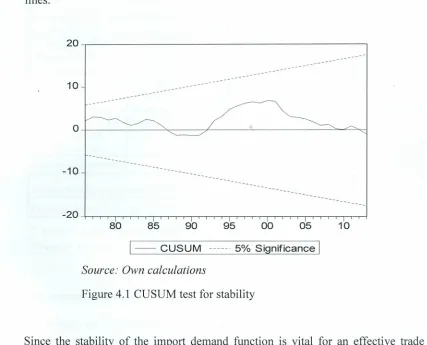
The CUSUM test (Brown, Durbin, and Evans, 1975) is based on the cumulative
sum of the recursive residuals and is used to test stability. This option plots the
cumulative sum together with the 5% critical lines. The test finds parameter
instability if the cumulative sum goes outside the area between the two critical
lines.
20~---.
10
o+---~----~---~---~~~
-10
80 85 90 95 00 05 10
1
--
CUSUM mm 5% SignificanceI
Source: Own calculations
Figure 4.1 CUSUM test for stability
Since the stability of the import demand function is vital for an effective trade
policy, testing whether the estimated import demand equation has shifted over
time is an important part of empirical studies. As showed by Figures 4.1 the
CUSUM test of parameter stability indicates that the parameters are stable during
the sample period. The findings are supported by Korean study on reexamination
4.7 Regression analysis
The results of regression analysis are presented in the table that follows.
Table 4.6 Regression results
Dependant variable Log of Value of imports
Variable Coefficient t-Statistic Prob.
Constant -1.661 -1.2l3 0.233
Log of Real
Gross Domestic
Product 0.378* 2.116 0.041
Log of Relative
pnce -0.026 -0.410 0.684
Log of Foreign exchange
reserve 0.159* 2.967 0.005
Lagged imports 0.726* 9.118 0.000
Adjusted R-squared 0.995 Schwarz criterion -0.884
Durbin-Watson stat 2.195 F- statistic 1860.9 p-value 0
*
implies that the coefficient is statistically significant at 5 percentSource: Own calculations L
The autonomous value of imports was -1.661. This was the value when all the
explanatory variables had a value of zero. The autonomous coefficient of the value
of imports was statistically insignificant with the probability value of 0.233.
Lagged value of imports was also a major determinant of imports (it had the
highest coefficient). Lagged value of imports coefficient was statistically
significant as the p-value was zero. Its coefficient was inelastic because it was
F-statistics showed that the variables included in the model were important
determinants of value of imports. Adjusted R-squared is 0.995. This means that
99.5 percent of change in value of imports is explained by variations in all the
explanatory variables included in the estimated model. The Durbin Watson is
2.195, which mean there is no autocorrelation.
4.8 Price Elasticity of Demand for Imports
The coefficient of price on imports had the expected negative sign according to the
traditional imports theory which was -0.0264. The coefficient of the variable was
statistically insignificant as the probability was 0.684 that is greater than 0.05. The
coefficient of price was inelastic. It means that 1 percent increase in price
decreases the value of imports decreases by 0.026 per cent. For China's aggregate
import demand, longrun price elasticities were found to be inelastic -0.52
(Moazzami and Wong, 1988), which was consistent with this study.
The non-significant or weakly significant relative price elasticities suggest that
devaluation and stablization policies pursued in the past did not effectively assist
trade liberalization efforts, at least at the rate they were implemented. More
generally, they suggest that policies that directly increase export earnings and
access to external capital inflows are likely to have a larger impact on import
volumes than those that concentrate exclusively on aggregate demand and
Heien (1968) aurged that for any country whose value of the price elasticity is
between 0.5 and -1.0 is necessary to ensure success of exchange depreciation.
Therefore, the estimated value of price elasticity 0.026 suggests that exchange rate
policy is found to be unfavorable in improving Kenya's trade balance in the long
run. Kenya has been pursuing a managed exchange rate regime with a view of
boosting exports and improving the current account position of the balance of
payments through maintaining competitiveness of its international market.
Moreover, the estimated long run relative price elasticity was inelastic. This
indicated that the value of imports demanded was insensitive to increases in
domestic price level.
4.9 Income Price Elasticity of Demand for Imports
The coefficient of real GDP was 0.378. The coefficient was statistically
significant considering the probability was 0.041. The coefficient of income was
inelastic because when the real GDP increases by 1 percent the value of imports
increases by 0.38 percent. The results indicate that import demand is inelastic with
respect to real income and thus submits that a growth income may not lead to the
expectation of trade deficits. The study for Indonesia supports this study (Dutta
and Ahmed, 1997). The estimated long-run income elasticity was closer to unity
(0.98) but inelastic still, and does suggest that Indonesia's import demand is
significantly driven by economic growth. If imports are biased towards imports of
consumption goods, ceteris paribus, the country may face problems in the balance
vanous final expenditures (real income) would seem most effective (Cheong,
2002).
4.10 Foreign Exchange Reserve Elasticity of Demand for Imports
The foreign exchange reserve elasticity of imports was 0.159. The coefficient was
statistically significant as its p value stood at 0.005. It was found to be inelastic as
one percent change in foreign exchange reserve caused 0.16 percentage increases
in import value. An increase in foreign reserves may have a positive effect on the
demand for imports since it relaxes the excess demand liquidity restriction.
Policies which focus on increasing foreign exchange reserves should be pursued,
CHAPTER FIVE
SUMMARY, CONCLUSION AND POLICY IMPLICATIONS
5.1 Introduction
Chapter five of the study contains summary of the study, conclusion, policy
implications and area for further research. Each part is discussed as follows.
5.2 Summary of the study
There is continued increase III imports volume and shrinking of exports. The
government was mostly preoccupied with mobilizing external financial assistance
and debt increased tremendously. The problem of growing population in Kenya,
heavy importing and borrowing lead to current account deficit. Information on
import demand elasticities is key to informing the tax policies that are to guide the
taxation of imports and deciding optimal imports. The specific objectives of the
study were to estimate income elasticity of demand for imports, price elasticity of
demand for imports and foreign exchange reserve elasticity of demand for imports.
Secondary data was used in the study and the period was from 1970 to 2013. Data
was collected from Central Bank of Kenya and Kenya National Bureau of
Statistics publications. A multiplicative import demand function was estimated
from which import elasticities were determined. The variables were found to be
co integrated in the long run.
The results show that income, relative price and foreign exchange reserve affect
imports value. Long run elasticities were estimated and the coefficients of the
statistically significant except relative price. The lag of value of imports was the variable with the highest coefficient and this indicated it drives Kenya imports. It was found that foreign exchange reserves matter for import demand in the long run. In addition, the sign of the estimated coefficient of reserves was positive, as expected. The statistical impact of foreign exchange reserve was significant.
5.3 Conclusion
The study concluded that the estimated coefficients for income, foreign exchange reserve and lagged value of imports are statistically significant except for relative price. All the coefficients had the expected signs. The value of imports was positively related to income, foreign exchange reserves and lagged imports and was found to be negatively related to relative prices. All coefficients of the variables were inelastic. Relative price coefficient was insignificant hence it could not be used to make any policy implications. There is unique long-run equilibrium relationship for Kenyan import demand. That is, income, foreign exchange reserve, lagged value of imports and prices are the plausible factors that affect import demand function
5.4 Policy Implications
Export promotion policies should be encouraged as they increase foreign exchange
reserves. This is because the results show that import demand respond to foreign
exchange reserve.
Exports are likely to increase foreign exchange reserves and can thereby provide
greater access to international markets which is in line with Vision 2030. This
policy is possible because foreign exchange reserve was positively related to
import demand.
Borrowing efforts should be discouraged given that foreign exchange reserves
elasticity was inelastic. This would improve balance of payments due to reduction
in debts.
Government can utilize imports of the previous period to forecast levels of tax
revenue and also determine import behavior. This was because the lagged value of
imports highly influences the demand of imports in Kenya.
5.5 Area for further research
Future research on the issue should also accompany disaggregated analysis of the
same. Another improvement in this regard would be to utilize the relative price
data of tradables versus the non tradables (instead of the commonly used practice
of using proxies). Further still, domestic absorption variable might be more
suitable instead of the real GDP for it would present the income minus the external
sector and would eliminate endogeniety that is inherent in the GDP and import
of various countries for comparative analysis and also towards employing a
R
EFERENCES
African Development Bank. (2012). African Economic Outlook Report. Kigali, African
Development Bank Group.
Arize .A and Osang, T. (2007). Foreign Exchange Reserves and Import Demand:
Evidence from
Latin America, Journal of Post Keynesian Economics, vol 9 No.4 pp 604 to 616.
Bertola,G., and Faini,R. (1991). Import demand and non-tariff barriers: The impact of
trade liberalization, Journal of Development Economics, 34: 269-286.
Brown RL, Durbin J, Evans JM (1975). Techniques for Testing the Constancy of
Regression Relationships over Time." Journal of the Royal Statistical Society B,
37: 149-163.
Caporale, Guglielmo Maria; Gil- Alana, Luis A; Mudida, Robert (2012). Testing the
Marshall-Lerner condition in Kenya, Discussion Papers, German Institute for
Economic Research, DIW Berlin, No. 1247.
Central Bank of Kenya .Quarterly Economic Reviews (various issues)
Dickey, D.A and Fuller, W.A (1981). Likelihood Ratio Statistics for Autoregressive Time
Series with a Unit Root, Econometrica, 49(4), pp.1057-1072
Dixit, A and Norman, V. (1980). Theory of International Trade, Cambridge: Havard
University Press.
Dutta, D. and. Ahmed (1997). An Aggregate Import Demand Function for Bangladesh: A
Cointergration Approach, Applied Economics, 31 (1991): 465-472.
Duesenberg, J. (1947). Income, Savings and the Theory of Consumer Behavior,
Cambridge
Egwaikhide, F.O. (1999). Determinants of Imports in Nigeria: A Dynamic Specification.
AERC Research Paper No. 91. African Economic Research Consortium, Nairobi.
Goldbrough, D.J (1981). International trade of multinational corporations and its
responsive to changes in aggregate demand and relative prices, IMF Staff papers,
28, pp.573-599.
Goldstein, M. and Khan17, M.S (1985). Income and Price Effects in Foreign Trade," in
Jones, R.W. and Kenen, P.B. (eds), Handbook of international Economics, 2, pp.
1041-1105, Elsevier.
Gross, M. and Elhanan, H. (1994). "Protection for Sale, American Economic Review, Vol
7 No.4 pp 883 to 850.
Gulhati, R. and et al (1985). Exchange rate policies in Eastern and Southern Africa, 196
5-83, WorldBankstaffworkingpaperNo. 720, World Bank, WashingtonD.C
Harvey. Sand Sedegah. K (2011), Import Demand in Ghana: Structure, Behaviour and
Stability, African Economic Research Consortium, Nairobi. Pp 25-27
Hemphill, W.L. (1974). The effects of foreign exchange receipts on imports of less
developed countries, IMF Staff Papers, 27: 637-77.
Heien, D.M. (1968). "Structural Stability and the Estimation of International Import Price
Elasticities in World Trade,"Kyklos, 21, 695-711.
Johansen, S (1998). Statistical analysis of cointegration vectors, Journal of Economic
Dynamics and Control, 12,pp 231- 254.
Khan, M.S. (1974). Import and export demand in developing countries". IMF Staff
Papers, 21 :678-693.
Khan, M.S. (1975). The structure and behaviour of imports in Venezuela, Review of