System Reduction of Discrete Time Uncertain Model using Stability Preservation Techniques

System Reduction of Discrete Time Uncertain

Model using Stability Preservation Techniques

Ankit Sachan

, Pankaj Kumar

, Dr.Pankaj Rai

Research Scholar, Dept. of EE, IIT (BHU) Varanasi, Varanasi, U.P., India1

Associate Professor, Dept. of EE, B.I.T. Sindri, Sindri, Jharkhand, India2

ABSTRACT: An e xtended approach for order reduction of co mple x discrete uncertain systems is prop osed. Using Interval arith metic Routh Stability arrays are formed to obtained numerator and denominator of reduced order model. The developed approach preserves the stability aspect of reduced system if higher order uncertain system is stable. A numerical e xa mple is included to illustrate the proposed algorithm along with the comparison with existing techniques . An extended technique for suppressing the comple xity of discrete time uncertain model using stability preservation approach is proposed. The numerator and denominator of uncertain mode l are suppressed by & table respectively. The proposed technique guarantees the preservation of stability in reduced uncertain model and we ll suited in quality with other e xisting methods. A numerica l illustration is discussed to exe mp lify the e xtended technique

KEYWORDS: Discrete Interval System, Integral Square Error (ISE), Model Order Reduction, Routh Stability Array.

I.INTRODUCTION

In present time as the comp le xity of physical and geo metrica l mode l increases many cases so it is desirable to represent reduced order system in place of its original system. System reduction for both continuous and discrete systems has been extensively studied. Conventional methods for system reduction are Aggregation method [1], Mo ment matching technique [2], Padé approximat ion [3], and factor division method [4]. Classical technique has many serious disadvantages which often lead to an unstable reduced order model even though the original system is stable. These drawbacks of c lassical techniques are overcome by stability preservation techniques which allows stable reduced model for stable system and having useful features such as the computational simplic ity and the fitt ing of time-mo ments. However, a p lenty of stability preservation techniques were developed in past. Some fa mous methods are Routh approximation [6], Stability equation method [7], table method [8], and many more.

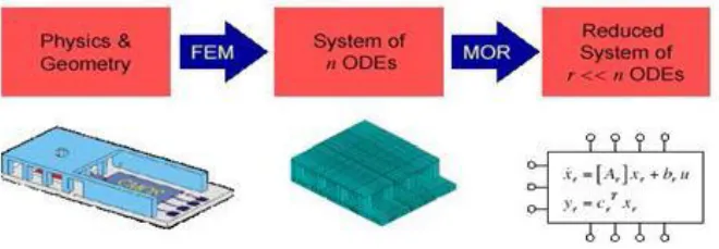
Fig 1. Order reduction of an efficient means to enable a system -level simu lation

Shaked [17] for discrete mu ltivariable system, Padè type approximat ions method [18] by Bandyopadhyay&Kande, bilinear Sch warz appro ximat ion [19] by Hsieh & Hwang etc. Apart fro m these, several techniques are proposed to check the novelty of reduced model.

In this brief, an extended technique is discussed for reduction of large system, where denominator is retained by  table of uncertain model while the numerator is obtained by  table of the given discrete interval system, This method shows the stability of the reduced system for a stable model. The outline of the paper is organized as follows: prima ries and main result of the paper are deliberated in Section II& III, Nu merical proble m is illustrated in Section III with the comparison of proposed result with other e xisting methods. Finally, conclusions and comments are given in Section IV.

II.PRIMALIES

A general higher order single input single output interval system of nth order is defined as 1

0 0 1 1 1 1

0 0 1 1

[ , ] [ , ] ... [ , ] ( ) [ , ] [ , ] ... [ , ] n n n n n n n

q q q q z q q z G s

p p p p z p p z

                     





 (1)

where (i=0,1,..., n-1) and (j=0,1,2,..,n) are order of interval para meters. and general reduced order system of rth order is defined as

1

0 0 1 1 1 1

0 0 1 1

[ , ] [ , ] ... [ , ] ( ) [ , ] [ , ] ... [ , ] r r r r r r r

b b b b z b b z R s

a a a a z a a z

                     





 (2)

where (i=0,1..., r-1) and (j=0,1,..., r) are order of interval para meters. Inter val Arithme tic [11, 12]

Rules based on interval arith metic [11, 12] a re given below. Let[ , ]a b and[ , ]c d be two intervals.

Addition: [ , ] [ , ] [a b  c d  a c b d,  ] (3)

Subtraction [ , ] [ , ] [a b c d  a d b c,  ] (4)

Multiplication [ , ] [ , ] [a b c d  Min ac ad bc bd( , , , )],[Max ac ad bc bd( , , , )] (5)

Div ision: [ , ] [ , ] [1 1, ] [ , ]

a b a b

c d   d c (6)

III. MAIN RES ULT

In this section Routh approximation based α- β table method [9] is extended for discrete uncertain system. The steps to obtain reduced order system are as below:

Step 1: Bilinear transformat ion of higher order system by applying 1

1 w z w   

Step 2: Recip rocal transformation of h igher order system is obtained as

ˆ_{( )} 1 ₍1 ₎

G w G

w w

 (7)

whereG wˆ ( )is reciprocal o f higher order system and G w( ) is the original higher order system

Step 3: Fo rmation of α -table

The first two rows of tabulation are formed fro m the coefficient of denominator of G wˆ ( )and rest of entries of table is by ―cross-multiplication ru le‖ using interval arith metic rules [11, 12] such as

    _ _ _{ } _ _       ] , ][ , [ ] , ][ , [ ] , [ ] , [ ] , [ 3 3 1 1 3 3 1 1 1 1 1 1 3 3 l l l l k k k k l l k k  









[ 1 1 1 1 2 2

            _{ } i i i i i

i k p p p p

k   ; i=(1,3,…, r-1)

] , ][ , [ ] , [ ] ,

[ 2 2 2 2 2 2

            _{ } i i i i i

i l p p k k

l   ; i=(1,3,…, r-3)

] , ][ , [ ] , [ ] ,

[ 2 2 3 3 2 2

            _{ } i i i i i

i m k k l l

m   ; i=(1,3,…, r-5)









Step 4: Fo rmation of β -table

The first two rows of table are formed fro m the coeffic ient of numerator of Gˆ(s) and remain ing entries are calculated fro m α table and earlier ro ws of β table

Therefore     _ _{ } _ _ _       ] , ][ , [ ] , ][ , [ ] , [ ] , [ ] , [ 3 3 1 1 2 2 0 0 1 1 0 0 1 1 p p p p q q q q p p q q       _ _ _ _ _ _       ] , ][ , [ ] , ][ , [ ] , [ ] , [ ] , [ 3 3 1 1 2 2 0 0 1 1 1 1 2 2 k k k k q q q q k k q q       _ _ _{ } _ _       ] , ][ , [ ] , ][ , [ ] , [ ] , [ ] , [ 3 3 1 1 3 3 1 1 1 1 1 1 3 3 l l l l e e e e l l e e  









[ 1 1 1 1 2 2

            _{ } i i i i i

i e q q p p

e   ; i=(1,3,…, r-3)

] , ][ , [ ] , [ ] ,

[ 2 2 2 2 2 2

            _{ } i i i i i

i f p p k k

f   ; i=(1,3,…, r-5)

] , ][ , [ ] , [ ] ,

[ 2 2 3 3 2 2

            _{ } i i i i i

i g r r l l

g   ; i=(1,3,…, r-7)









Step 5: Let Ar(s) and Br(s) represent the denominator and numerator respectively, of the rth order reduced system in

general [19], i.e.

) ( ) ( ] , [ )

(s A 1 s A 2 s

Ar r r r r



 _

   (8)

] , [ ) ( ) ( ] , [ )

( 1 2

      _{ }

 _{r r r r r r}

r s sB s B s

B     (9)

Where r =(1, 2, ..., n)are obtained with _{( ) 0}

1 

 s

A , _{( ) 0}

1 

 s

B , _{( ) 1}

0 s 

A , _{( ) 0}

0 s 

B ;

Step 6: The rth order rec iprocal t ransformat ion system is evaluated as

) ( ) ( ) ( ˆ s A s B s R r r

r  ₍₁₀₎

Step 7: Finally reduced order system is obtained as

) 1 ( ˆ 1 ) ( s R s s

Rr  r (11)

Step 8: Inverse Bilinear transformation of reduced order system by applying 1

IV. NUMERICAL EXAMPLE

Consider the fourth order discrete interval system described by transfer function [27, 28]

2

3 2

[1, 2] [3, 4] [8,10] ( )

[6, 6.6] [9,9.5] [4.9,5] [0.8, 0.85]

z z G z

z z z

 



  

Step 1: Applying bilinear transformation in h igher order transfer function. 2

3 2

[5,9] [ 18, 12] [12,16]

( )

[0.55,1.2] [5.9, 6.65] [19.45, 20.2] [20.7, 21.35]

w w

G w

w w w

   



  

Step 2: After recip rocal transformation of G(s) 2

3 2

[12,16] [ 18, 12] [5,9]

ˆ ( )

[20.7, 21.35] [19.45, 20.2] [5.9, 6.65] [0.55,1.2]

w w

G w

w w w

   



  

Step 3: The table is obtained as:

table



[19.45, 20.2] [0.55,1.2] [1.024,1.097] [4.583,6.0864]

[3.1956, 4.407]

Step 4: The β table is calculated as:

table

  [12,14] [5,9]

[ 18, 12]  [0.59,0.82] _{[6, 7.5]} [ 2.95, 2.62] 

Step 5: Now transformation reduced system, using Eq.10 is evaluated as

2 2

[1.88,3.60] [ 2.95, 2.62] ˆ ( )

[3.25, 4.79] [3.19, 4.40] 1

w R w

w w

  



 

Step 6: Then, reciprocal transformation of above reduced order system using Eq. 11 is obtained as

2 2

[ 2.95, 2.62] [1.88,3.60] ( )

[3.19, 4.40] [3.25, 4.29]

w R w

w w

  



 

Step 7: Applying inverse bilinear transformation in reduced order transfer function as

2 2

[ 1.07, 0.98] [4.5, 6.55] ( )

[7.44,10.19] [4.5, 7.58] [ 0.15, 2.6]

z R z

z z

 



  

V. RES ULT AND DISCUSS ION

To check the superiority of the proposed method over other existing methods [27, 28] integral-square-error fo r reduced order models are tabulated in Table I. The integral square error is determined between transient step response of original system and its reduced order model which can be represented as

dt t y t y ISE r

2

0[ () ()]





(12)

TABLE I. COMPARISON OF ISE FOR REDUCED ORDER MODELS

Model Order Reduction Reduced Models ISE

(lower)

ISE (upper)

Proposed Method ₂

2

[ 1.07, 0.98] [4.5, 6.55] ( )

[7.44,10.19] [4.5, 7.58] [ 0.15, 2.6]

z G z

z z

 



   0.0852 0.0377

Padé& Dominant Pole

Retention Method [27] 2 2

[0.5921, 0.6055] [0.8845, 0.9] ( )

[0.8041,1.2465] [0.1437, 0.3805]

z G z

z z

 

  0.1810 0.0.741

  method [28] ₂

2

[ 1.328,1] [3.522,5.85] ( )

[6.89,8.14] [3.94,5.44] [0.55,1.8]

z G z

z z

 



  1.1292 0.0443

Fig 1(a). Step response of Original and reduced systems using Kharitonov‘s theorem

Fig 1(b). Step response of Original and reduced systems using Kharitonov‘s.theorem

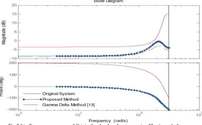
Fig 2(a). Frequency response of Original and reduced systems using Kharitonov‘s theorem

Fig 2(b). Frequency response of Original and reduced systems using Kharitonov‘s theorem

In the fig 2(a) & fig 2(b), it shows the frequency response of higher order system and lowe r order systems using Kharitonov‘s theorem in which g raph is shown for magnitude (dB) & phase (deg) Vs time (seconds).

VI.CONCLUS ION

This paper presents an extension of the α- β table technique [13] for reduction of higher order discrete time interval systems. The numerator polynomial and denominator polynomial is obtained by using β table and α table respectively. The developed technique is conceptually easy and preserves the accuracy and stability of reduced order model if the higher order system is stable. The proposed method produces lesser values of error indices when compared with other e xisting methods [27,28]. A nume rica l e xa mp le is discussed and compared with some e xisting techniques.

REFER ENC ES

[1] M. Aoki, ―Control of large-scale dynamic systems by aggregation,‖IEEE Trans. Automat. Contr., vol. AC-13, pp. 246-253, 1968. [2] N. K. Sinha and B.Kuszta, ― Modeling and identification of dynamic systems,‖ New York: Van Nostand Reinhold, pp.133-163, 1983 [3] Y. Shamash, ―Stable reduced order models using Padè type approximation,‖ IEEE T rans. Automat. Contr., vol. AC-19, pp. 615-616, 1974. [4] T.N. Lucas, Factor division: a useful algorithm in model reduction, IEE Proc. 130, Vol. 6, 362–364, November 1983.

[6] V. Krishnamurthy and V. Seshadri, ― Model reduction using the Routh Stability criterion,‖IEEE Trans. Automatic Control, vol. AC-23, pp.729– 731, Aug. 1978.

[7] T.C. Chen, C.Y. Chang, and K.W. Han, ―Stable reduced-order Padè approximants usingstability equation method,‖ Electron. Lett., 1980,16, pp. 345–346.

[8] M.F. Hutton and B. Friedland, ― Routh Approximation for Reducing Order of Linear T ime Invariant System‖, IEEE Trans. Autom. Control,20, 329-337, 1975

[9] R.K. Appiah,―Padè methods of Hurwitz polynomial approximation with application to linear system reduction,‖ Int. J. Control, 1979, 29,pp. 39–48.

[10] K. Glover, ―All Optimal Hankel-norm Approximations of Linear Multivariable Systems andtheir L∞ Error Bounds," International Journal of Control, pp. 1115-1193, vol. 39 (6), 1984.

[11] E. Hansen, ―Interval arithmetic in matrix computations—Part I,‖ SIAMJ. Numerical Anal., pp. 308–320, 1965 [12] E. Hansen and R. Smith, ―Interval arithmetic in matrix computation.Part II,‖ SIAM J.Numerical Anal., pp. 1-9, 1967

[13] M. Sharma, A. Sachan, D. Kumar, "Order reduction of higher order interval systems by stability preservation approach," inPower, Control and Embedded Systems (ICPCES), 2014 International Conference on , vol., no., pp.1-6, 26-28 Dec. 2014

[14] V. L. Kharitonov , ―Asymptotic stability of an equilibrium position of a family of systems of linear differential equations,‖ Differentsial'nye Uravneniya, 14, pp.2086-2088, 1978.

[15] R. Barmish, ―A generalization of Kharitonov‘s four polynomials concept for robust stability problems with linearly dependent coefficient perturbation,‖ IEEE Tran. Auto. Cont., vol. 31, No. 2, pp. 157-165, 1989.

[16] Y. Shamash, and D. Feinmesser, ‗Reduction of discrete time systems using a modified Routh array‘, International Journal of Sy stem Science, vol. 9, no. 1, pp. 53-64, 1978.

[17] Y. Bistritz;U. Shaked.".Discrete multivariable system approximations by minimal Pade-typestable models". IEEE Transactions on Circuits and Systems,Volume: 31 ,Issue: 4 , Page(s):382 - 390,1984.

[18] P. Parthasarthy and K. N. Jayasimha, ‗Modeling of Linear Discrete-Time Systems usingModified Cauer Continued Fraction‘. Journal of Franklin Inst, vol. 316, no. 1, pp. 79, 1983.

[19] Bandyopadhyay and Kande (1988) proposed a method of model reduction for discrete-timecontrol systems by Pade type approximations. [20] Y. Choo, ‗A Note on Discrete Interval System Reduction via Retention of Dominant Poles‘,International Journal of Control, Automation, and

Systems, vol. 5, no. 2, pp. 208-211, 2007.

[21] N. Pappa and T. Babu, ‗Biased model reduction of discrete interval system by differentiationtechnique‘, Annual IEEE India Conference, (INDICON), pp. 258 – 261, 2008.

[22] B. Vishwakarma, and R. Prasad, ‗Clustering method for reducing order of linear systemusing Pade approximation‘, IETE Journal of Research, vol. 54, no. 5, pp. 326-330, 2008.

[23] S. K. Mittal, and D. Chandra, ‗Stable optimal model reduction of linear discrete time systemsvia integral squared error minimization: computeraided approach‘, Jr. of Advanced Modelingand Optimization, vol. 11, no. 4, pp. 531-547, 2009.

[24] V. P. Singh and D. Chandra, ‗Model reduction of discrete interval System using dominantpoles retention and direct series expansion method‘, The 5th International Power Engineering and Optimization Conference (PEOCO), pp. 27-30, 2011.

[25] Hwang, C., and Hsieh, C.S., ―Order reduction discrete time system viz., Bilinear RouthApproximation‖, ASME J. Dyn, Syst, Meas., control 112, PP 292 – 297, 1990.

[26] M. F. Hutton, ―Routh approximation method for high-order linear systems,‖ Ph. D. dissertation, Polytechnic Inst. New York, Brooklyn, N.Y., June 1974.

[27] O. Ismail, B. Bandyopadhyay, and R. Gorez, ―Discrete interval system reduction using Padé approximation to allow retention of dominant poles,‖ IEEE Trans. on Circuits and Systems-I: Fundamental theory and applications, vol. 44, no. 11, pp. 1075-1078, 1997.