ISSN 2286-4822 www.euacademic.org
Impact Factor: 3.4546 (UIF) DRJI Value: 5.9 (B+)
Estimating the Effect of the Shape Parameter for
Probability Distribution Using the Minimum
Variance Method
Dr. HAMZA IBRAHIM HAMZA Faculty of Urban Sciences Al - Zaeem Al - Azhari University
Abstract:
Key words: effect of the shape parameter, probability distribution, minimum variance method
Introduction:
The estimation of descriptive statistical measures in terms of one of the random samples taken is one of the main reasons for analysis and decision-making. Two types of estimates can be distinguished: the point estimate is only one value for the statistical constant estimated in terms of the corresponding statistical factor, calculated from the random sample drawn from the society The estimate is to estimate the value of the statistical constant within a given field at a given probability in terms of the corresponding statistical function. Those hard into account the value of the standard error of the estimate continued to be the statistical Bdalalth value we get edged located between the highest and lowest of the most important reasons that help in the study of sampling theory is the desire to obtain information about the required study of society.
The Study Problem:
When using any method of estimation, it is necessary to find the best estimate of the characteristics of the society to be estimated so that they are close to the estimate with the least error, since there is a set of distributions used in applied research.
1. What is the best estimate of the least error to estimate the shape parameter of the distributions?
2. Is it possible to know the best estimate of a distribution parameter by comparing several estimates using the least variance method?
The Importance of Studying:
The importance of the study was as follows:
1. To emphasize the importance of compiling the data in the sizes of different samples and different probability distributions with different shape parameters, in order to avoid any problems that researchers may encounter when conducting their research on real data.
2. The importance of using the sample data in estimating the parameters of the shape of binomial, bias one and natural distributions. They used the least variance method to find out the effect of this method on the shape parameter in terms of good estimation.
3. Estimation of the point is the best estimate of the community parameter and it is the basis of the estimation process in the period and the tests of hypotheses.
Objectives of the Study:
The objectives of the study were as follows:
1. Recognition of the values of the parameters of the shape of binomial, bias one and natural distributions, using the maximum potential method.
2. Recognition of the criterion of differentiation to estimate the shape parameter in the manner of the lowest variance between binomial, bias one and natural distributions.
3. To arrive at the best estimate of the shape parameter when it is small, medium and large for binomial, bias one and natural distributions so that this estimate is as close as possible to the value of the shape parameter of the distribution concerned.
Methodology Of The Study:
The descriptive approach was followed with regard to the theoretical aspect of the subject of the study. As for the applied side, the case study was used to generate the sample data by the simulation method. The data were generated by binomial, Poisson, Norma, gamma distributions. Using the Mental program
Simulation style:
finding the means by which the researcher can study the problem and analyze it despite the difficulties in expressing it in mathematical model(4).
The simulation of the real system is carried out by a theoretically predictable system of behavior through a specific probability distribution. Thus, a sample of this system can be sampled by so-called random numbers ( 5).
Simulation is defined as a numerical technique used to perform tests on a numerical computer that includes logical and mathematical relationships that interact with each other to describe the behavior and structure of a complex system in the real world and are finally described as the process of creating the spirit of reality without achieving this reality at all(4)..
The Concept of Monte Carlo Model:
The basis of this model is the selection of the hypothesis elements available (probability) by taking random samples and can be summarized in the following steps (6):
1. Determine the probability distribution for each variable in the model to be studied.
2. Use random numbers to simulate probability distribution values for each variable in the previous step.
3. Repeat the process for a set of attempts.
Random Numbers:
Is the number was chosen by random quantity operation and random numbers are used to generate simulation values for many probability distributions. There are many ways to generate random numbers such as linear matching, use random number tables, and use functions ready for this purpose, such as the Rand function used in many programming languages (1).
Maximum Variance (4):
Is one way of estimation, let(x) be a random variable with a probability block functionp(x) ، Which requires the estimation of any
random variables for the estimation process, provides
a method for estimating the least variation on the following formula:
θ (θ) *θ̂ θ+ where :
The maximum likelihood function . θ̂
(θ)
(θ) θ̂ Ie do not rely on sample data.
(θ) (θ)
In this way, unbiased estimates of the least variance and sufficient and necessary condition for the existence of an unbiased estimate with the least variation such as x are the possibility of forming the first partial derivative of the function of the distribution function (function) as follows (5):
θ
It is then said that is an unambiguous estimate with the least
variance of parameter and that represents the variance of this estimate.
Binomial distribution (7):
The binomial distribution is one of the intermittent distributions of great practical importance in the randomized experiments that result in one of two outcomes: the initial name - the desired success and the other the non-required failure. This distribution was discovered in 1700 by the world (James Bernolli)
It is said that the variable x follows binomial distribution with( ) parameters if its probability attribute is:
This distribution is represented by the symbol .
Estimating the shape parameter of the Binomial distribution in the minimum variance method:
∑
∑
And the unification of denominations :
∑ ∑
∑ ∑ ∑
∑ ∑ ∑
∑
But ∑ : By divided on
And compared to the equation
θ
is being:
̂
Characteristics of Distribution:
1. Mean E(X)
2. Variance V(X)
Poisson distribution)1):
Is a probability distribution that is used to calculate the probability of a certain number of successes (x) in a unit of time or in a given area when events or successes are independent of one another and when the average of success remains constant for the unit of time. By the world (Poisson).(1)
If (x) random variable follows the Poisson distribution with parameter λ, its probability function is:
Where :
X number of successes.
P (X = x) The probability of the given number of successes taking the value x
The basis of the natural logarithmic system e = 2.71828 This distribution is represented by the symbol X ~ Pos (λ).
Estimating the shape parameter of the Poisson distribution in the least contrast method:
When estimating the Poisson distribution parameter in the greatest possible way:
∑
The unification of denominators:
∑
By dividing :
∑
And compared to the equation: θ is being:
̂
Characteristics of Distribution:
1. Mean E(X)
2. Variance V(X)
Normal Distribution (2):
Is one of the most frequent and most widely used probability distributions. It plays a major role in statistical theory and probability theory. This distribution was called normal distribution (or moderate or normal) because it was previously thought that any data on life should be represented and subject to this distribution, but it is now proven that this is not the case and that the belief is wrong. It is also known as the Gauss distribution, thanks to the German scientist Frederick Gauss, who developed mathematical distribution as a probability distribution in the year (1855-1777)
distribution curve approaches the horizontal axis but never touches it.(2)
If x is a random variable connected to a natural distribution of the parameters (μ, σ), the distribution function is:
√
( )
Where:
f (X) natural curved height.
The mean of the distribution
Standard deviation
The basis of the natural logarithmic system e = 2.71828.
Constant ( =3.14159).
This distribution is denoted by X ~ N (μ, σ)
Estimating the parameters of the shape and measurement of natural distribution in the greatest possible way (7):
When estimating the normal distribution parameter (μ) in the greatest possible way
∑
∑
By dividing and by the equation: θ is being:
∑
∑
∑
∑
∑
-
And the unification of denominators:
∑
By dividing n:
∑
And compared to the equation:
θ
is being:
∑
Characteristics of Distribution:
1. Mean E(X)
2. Variance V(X)
Gamma Distribution (2):
It is used to study the time between the arrival of words to a particular service center, such as the arrival of the baker to a bank or the entry of patients to the hospital. A function known as Γα ) As follows (3):
1. If n is positive, the integration is approximated and is: i. Γ (1) = 1
ii. Γn = (n-1) Γ (n-1)
2. If n is a positive integer, then:
∫
∫
The general picture of the distribution is:
Estimation of two distribution parameters in the least variance method (7):
To obtain an estimate of the measurement parameter (α) and the parameter of the form (β) for the distribution in the least variance method follow the following steps:
When estimating the distribution of teachers in the greatest possible way we find that:
̂
̂ ̂
And the unification of denominators and By dividing on ( ̂(
̂ ̂ ̂
̂̂
And compared to the equation
θ
is being :
̂ ̂
̂ ̂ ̂
Characteristics of Distribution:
1. Mean E(X)
Materials and Methods of Research:
Distributed tracking data was generated using the Minitab program as follows:
1. Generation of the size of society M from binomial distribution X ~ B (n, P) with knowledge of n, P and distribution of Poisson X ~ Pos (λ) by λ and normal distribution X ~ N (μ, σ) And the distribution of X ~ Gamma (α, β) by (α, β).
2. Choose the sample size n and denote it with the symbol j. 3. Determination of parameters for both binomial distribution,
Poisson, natural, and gamma. 4. Repeat steps 1-3 of j = 1,2,3
Monte Carlo simulation results:
Distributed tracking data has been generated as follows:
Generate data for binomial distribution with sample sizes 10, 30, 50 and 70 and with parameter P are 0.3, 0.5, 0.7 and 0.9 and n parameter, B10.
And generate Poisson distribution trace data with sample sizes 10, 30, 50 and 70 and with parameter, λ are 0.3, 0.5, 0.7 and 0.9. And generate natural distribution tracking data with sample sizes 10, 30, 50 and 70 and with the parameter, σ 0.3, 0.5, 0.7 and 0.9 and the parameter μ (10).
And generate distribution trace data with sample sizes 10, 30, 50 and 70, with a parameter of α is 0.3, 0.5, 0.7, 0.9 and β parameter (10).
ANALYSIS, INTERPRETATION, AND DISCUSSION:
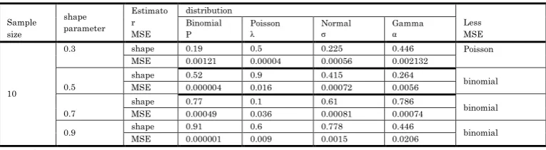
Table (1): Determination of the shape parameter for probability distribution with parameter (0.3), (0.5), (0.7) and (0.9) and sample size (10) Less MSE distribution Estimato r MSE shape parameter Sample
size Gamma α
Normal σ Poisson λ Binomial P Poisson 0.446 0.225 0.5 0.19 shape 0.3 10 0.002132 0.00056 0.00004 0.00121 MSE binomial 0.264 0.415 0.9 0.52 shape
0.5 MSE 0.000004 0.016 0.00072 0.0056
binomial 0.786 0.61 0.1 0.77 shape
0.7 MSE 0.00049 0.036 0.00081 0.00074
From Table (1) we find that at the sample size 10 and the parameter of Fig. 0.3, the estimation of the shape parameter using the float method is best when parsing the Poisson because the estimated value of 0.5 is the appropriate and close to the value of the parameter of figure 0.3 and the lowest average error box MSE is equal to 0.00004 , We find that at the size of sample 10 and the parameter of Fig. 0.5, 0.7 and 0.9, the estimation of the shape parameter using the zoom method is preferable for binomial distribution because the estimated values are close to the parameter values of the shape and the mean error box MSE is equal to 0.000004 and 0.00049 and 0.000001 respectively.
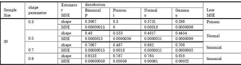
Table (2): Determination of the shape parameter for probability distribution with parameter (0.3), (0.5), (0.7), (0.9) and sample size (30)
Less MSE distribution Estimato r MSE shape parameter Sample Size Gamma α Normal σ Poisson λ Binomial P Poisson 0.286 0.3731 0.3 0.3067 shape 0.3 30 0.0000006 0.00018 0 0.00000015 MSE Normal 0.4454 0.4817 0.533 0.48 shape
0.5 MSE 0.0000013 0.0000036 0.0000011 0.0000099
binomial 0.708 0.682 0.467 0.7067 shape
0.7 MSE 0.00000015 0.0018 0.0000011 0.0000002
binomial 0.818 0.765 0.767 0.9133 shape
0.9 MSE 0.00000059 0.00059 0.00061 0.00022
Source: The Researcher By Minitab
Table (3): Determination of the shape parameter for probability distribution with the parameter of (0.3), (0.5), (0.7) and (0.9) and sample size (50)
Less MSE distribution Estimator MSE shape parameter Sample size Gamma α Normal σ Poisson λ Binomial P Normal 0.3107 0.1985 0.24 0.296 shape 0.3 50 0.0000002 0.00015 0.0000072 0.000000032 MSE binomial 0.581 0.3357 0.66 0.49 shape
0.5 MSE 0.0000006 0.000512 0.00039 0.00013
Gamma 0.705 0.731 0.52 0.658 shape
0.7 MSE 0.0000035 0.00065 0.0000014 0.00000005
binomial 0.857 0.942 1.000 0.926 shape 0.9 0.0000037 0.0000025 0.0002 0.0000014 MSE
Source: The Researcher by Minitab
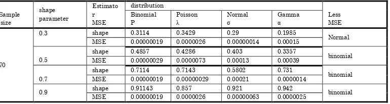
Table (4): Determination of the shape parameter for probability distribution with the parameter of (0.3), (0.5), (0.7) and (0.9) and sample size (70)
Less MSE distribution Estimato r MSE shape parameter Sample size Gamma α Normal σ Poisson λ Binomial P Normal 0.1985 0.29 0.3429 0.3114 shape 0.3 70 0.00015 0.00000014 0.0000026 0.00000019 MSE binomial 0.3357 0.403 0.4286 0.4857 shape
0.5 MSE 0.00000029 0.0000073 0.00013 0.00039
binomial 0.731 0.5802 0.7143 0.7114 shape
0.7 MSE 0.00000019 0.00000029 0.00021 0.0000014
binomial 0.942 0.921 0.857 0.91143 shape 0.9 0.0000025 0.00000063 0.0000026 0.00000019 MSE
Source: The Researcher by Minitab
From Table (4) we find that at the sample size 70 and the parameter of Fig. 0.3, the estimation of the shape parameter using the zoom method is better at the normal distribution because the estimated value of 0.29 is close to the value of the parameter of figure 0.3 and the lowest average error box MSE is equal to 0.00000014, That at the sample size 50, 0.7 and 0.9, the estimation of the shape parameter using the zoom method is preferable for binomial distribution because the estimated values are close to the parameter values of the shape and the mean error box MSE is equal to 0.00000029, 0.00000019 and 0.00000019, respectively.
We deduce from the above that for estimating the small shape parameter (0.3) at the size of sample 70 for binomial, bias one and natural distributions, they can use the estimation method for normal distribution because it is better for normal distribution than distributions. The estimation of the shape parameter using the zoom method is best for binomial distribution because the estimated values are close to the parameter values of the binomial distribution
RESULTS:
1. For the size of the sample (10) to estimate the small shape parameter (0.3) for binomial and Poisson distributions, and natural, they can use the Poisson distribution because it is the best among the distributions. To estimate the parameter of the figure (0.5), (0.7) ), The binomial can be used because it is preferable to double-edged distributions. 2. In the sample size (30) to estimate the small shape
natural, they can use the Poisson distribution because it is the best among the distributions. Among the distributions, and to estimate the shape parameter (0.7), (0.9), the binomial distribution can be used because it is the best among the distributions.
3. In the sample size (50) for estimating the small shape parameter (0.3) for the binomial distribution and Poisson and natural, they can use the normal distribution because it is the best among the distributions. Among the distributions, and to estimate the parameter of the figure (0.5), (0.9), the binomial distribution can be used because it is the best among the distributions.
4. In the sample size (70) for the estimation of the small shape parameter (0.3) for the binomial distributions and Poisson and natural, they can be used for normal distribution because it is the best among the distributions. To estimate the parameter of the figure (0.5), (0.7) ), The binomial can be used because it is preferable to double-edged distributions.
RECOMMENDATIONS:
1. Use a binomial distribution to estimate the shape parameter (0.9) at sample size (10), (30), (50), (70).
2. Expand the study of a number of other community distributions. 3. Application of a number of estimation methods for binomial
distributions, Poisson, natural.
REFERENCES:
1. Adnan Abbas Humaidan, Matanios Makhoul, Farid Ja'ouni, Ammar Nasser Agha (2015-2016) Applied Statistics Faculty of Economics, University of Damascus.
2. Ahmed Hamad Nouri, Ihab Abdel-Rahim Al-Dawi (2000).
4. Hossam Bin Mohammed The Basics of Computer Simulation (King Fahd National Library, Al Rayah, 2007).
5. Jalal al-Sayyad Statistical Inference
6. Nutrition and simulation Dr. Adnan Majed Abdulrahman (King Saud University 2002).