Delay Extraction based Macromodeling with Parallel Processing for Efficient Simulation of High Speed Distributed Networks

Scholarship@Western

Scholarship@Western

Electronic Thesis and Dissertation Repository

7-2-2013 12:00 AM

Delay Extraction based Macromodeling with Parallel Processing

Delay Extraction based Macromodeling with Parallel Processing

for Efficient Simulation of High Speed Distributed Networks

for Efficient Simulation of High Speed Distributed Networks

Sourajeet Roy

The University of Western Ontario

Supervisor

Dr. Anestis Dounavis

The University of Western Ontario

Graduate Program in Electrical and Computer Engineering

A thesis submitted in partial fulfillment of the requirements for the degree in Doctor of Philosophy

© Sourajeet Roy 2013

Follow this and additional works at: https://ir.lib.uwo.ca/etd

Part of the Electrical and Electronics Commons, and the VLSI and Circuits, Embedded and Hardware

Systems Commons

Recommended Citation Recommended Citation

Roy, Sourajeet, "Delay Extraction based Macromodeling with Parallel Processing for Efficient Simulation of High Speed Distributed Networks" (2013). Electronic Thesis and Dissertation Repository. 1327.

https://ir.lib.uwo.ca/etd/1327

This Dissertation/Thesis is brought to you for free and open access by Scholarship@Western. It has been accepted for inclusion in Electronic Thesis and Dissertation Repository by an authorized administrator of

Delay Extraction based

Macromodeling with Parallel

Processing for Efficient Simulation

of High Speed Distributed

Networks

(Thesis format: Monograph)

by

Sourajeet Roy

Graduate Program in Engineering Science

Department of Electrical and Computer Engineering

A THESIS SUBMITTED IN PARTIAL FULFILLMENT OF THE REQUIREMENTS FOR THE DEGREE OF DOCTOR OF PHILOSOPHY

The School of Graduate and Postdoctoral Studies The University of Western Ontario

ii

With the increase in signal speeds in VLSI systems, distributed effects arising in passive

components such as high speed interconnects and power distribution networks are the main

contributors of signal and power degradation at chip, package and board levels. As a result,

computer aided design strategies targeting modeling and simulation of such high speed

systems at the early design stages are critical requirements for VLSI designers. However, the

computational demand of accurately capturing the distributed nature of such components is a

major bottleneck facing traditional circuit solvers.

This thesis deals with two different approaches towards modeling of high speed distributed

networks. One approach deals with cases where the physical characteristics of the network

are not available and the network is characterized by its frequency domain, multiport

tabulated data. The other approach is based on a detailed knowledge of the physical and

electrical characteristics of the network and assuming a quasi transverse mode of propagation

of the electromagnetic wave through the network.

In the first part of the thesis, a delay extraction based IFFT algorithm is described for the

accurate macromodeling of electrically long interconnect networks characterized by its

frequency domain, multiport Y parameter data. An important feature of this work is the ability to extract the higher order delays and the associated attenuation losses embedded in

the data via time-frequency decompositions. The effect of including the higher order delays

have been shown to lead to greater accuracy over existing direct IFFT or even single delay

iii

package/board level power distribution networks (PDNs) where prior knowledge of the

physical and electrical characteristics of the network is readily available. The proposed

macromodeling technique is based on a delay extraction feature and has been readily applied

to two dimensional (2D) and three dimensional (3D) PDNs with irregular geometries. The

key advantage of the algorithm is that through explicit delay extraction, the distributed nature

of the PDNs can be accurately captured, leading to more compact and more accurate

broadband simulation of the network as compared to traditional lumped modeling

approaches.

Finally, waveform relaxation (WR) based algorithms for parallel simulations of large

multiconductor interconnect networks and 2D PDNs are presented. A key contribution of

this body of work is the identification of naturally parallelizable and convergent iterative

techniques that can divide the computational costs of solving such large macromodels over a

multi-core hardware. Additional techniques to accelerate convergence, reduce the simulation

cost per iteration as well as communication overheads among the cores have been described.

Numerical examples are provided to illustrate the superior scalability of the proposed

algorithm with respect to the size of the network and available parallel processors when

compared to conventional sequential modeling approaches.

Keywords: Convergence, Delay extraction, Electromagnetic interference, High speed

interconnects, Iterative algorithms, Macromodeling, Multiconductor transmission lines,

Parallel processing, Power distribution networks, Power integrity, Signal integrity,

iv

This thesis could not be successful without the invaluable support of my supervisor Dr.

Anestis Dounavis of the Department of Electrical and Computer Engineering at University

of Western Ontario. I would like to express my gratitude towards him for introducing me to

the area of computer aided design for VLSI applications and inculcating in me the

enthusiasm for research. His motivation, keen acumen in this field of research and friendly

disposition has always been a major motivation for my work.

I would also like to extend my thanks towards every faculty member, staff member and

friend of the Department of Electrical and Computer Engineering, Western University for

their support and help at various stages of my thesis work. I would like to specially mention

my colleagues Dr. Majid Ahmadloo, Dr. Amir Beygi and Dr. Ehsan Rasekh for their

invaluable advice and inspiration.

In addition, I would like to thank my parents, Mr. Tarit Kanti Roy and Mrs. Shanghamitra

Roy for their blind faith in my scholarly ability even when it was convenient not to. I would

also like to thank my sister Dr. Sohinee Roy for being the loudest cheerleader for me. She

has taught me that every obstacle is just a detour, not a dead end. Finally, this thesis would

have been impossible without the presence of my dearest friend, Ms. Alka Grover. Despite

the miles separating us, her support and faith has been a torch that I carried through the best

v

Abstract ... ii

Acknowledgments... iv

Table of Contents ... v

List of Tables ... ix

List of Figures ... x

Abbreviations ... xv

Chapter 1 ... 1

1 Introduction ... 1

1.1 Background and Motivation ... 1

1.2 Objectives and Contributions ... 5

1.3 Organization of the Thesis ... 7

Chapter 2 ... 9

2 Background and Literature Review ... 9

2.1 Introduction ... 9

2.2 Macromodeling based on Measured Data ... 10

2.3 Macromodeling of Power Distribution Networks... 13

2.3.1 Single Layered PDNs ... 15

2.3.2 Multilayered PDNs………16

2.4 High Speed Interconnect Modeling ... 20

2.5 Simulating Interconnects in SPICE-like Simulators………..22

2.5.1 Lumped Segmentation ... 22

2.5.2 Matrix Rational Approximation ... 23

vi

2.5.5 Transmission Line Macromodels with Incident Fields ... 29

2.6 Waveform Relaxation for Parallel Simulation ... 30

2.6.1 Optimization based LP-WR ... 32

2.6.2 MoC based LP-WR………33

Chapter 3 ... 35

3 Transient Simulation of Distributed Networks using Delay Extraction based Numerical Convolution……….35

3.1 Introduction ... 35

3.2 Motivation and Review of Time-Frequency Decompositions ... 36

3.2.1 Motivation ... 36

3.2.2 General Time-Frequency Decompositions ... 37

3.3 Development of the Proposed Algorithm ... 39

3.3.1 Determining Multiple Delays (TK) ... 39

3.3.2 Partitioning the Time-Frequency Plane ... 42

3.3.3 Computing the Attenuation Losses (Yij(k)(s)) ... 43

3.4 Numerical Examples ... 45

3.5 Conclusion ... 53

Chapter 4 ... 54

4 Delay Extraction based Macromodeling of Power Distribution Networks ... 54

4.1 Introduction ... 54

4.2 Development of the Proposed Macromodel ... 55

4.2.1 Formulation of Transmission Line Model for PDN………..55

4.2.2 Modeling Unit Cells using DEPACT ... 59

4.2.3 SPICE Realization of Lossy Section... 60

vii

Chapter 5 ... 71

5 Longitudinal Partitioning based Waveform Relaxation Algorithm for Efficient Analysis of Distributed Transmission Line Networks ... 71

5.1 Introduction ... 71

5.2 Overview of Waveform Relaxation Algorithms ... 72

5.3 Development of the Proposed Waveform Relaxation Algorithms ... 73

5.3.1 Proposed Partitioning Scheme for MTLs ... 74

5.3.2 Iterative Solution of Subcircuits using Gauss-Jacobi ... 76

5.3.3 Hybrid Iterative Solution of Subcircuits ... 77

5.4 The Computational Complexity of the Proposed Algorithm ... 80

5.5 Numerical Results ... 84

5.6 Conclusion ... 90

Chapter 6 ... 91

6 Electromagnetic Interference Analysis of Multiconductor Transmission Line Networks using Longitudinal Partitioning based Waveform Relaxation Algorithm ………91

6.1 Introduction ... 91

6.2 Background of EMI Analysis of MTL Networks ... 93

6.2.1 General Formulation of MTLS Exposed to Incident EM Fields ... 93

6.2.2 DEPACT Model for EMI Analysis... 95

6.3 Development of the Proposed WR Algorithm ... 98

6.3.1 Generation of Compact Subcircuits ... 98

6.4 Numerical Examples ... 103

6.5 Conclusion ... 108

Chapter 7 ... 109

viii

7.2 Development of the Proposed WR Algorithm ... 111

7.2.1 Proposed 2D Partitioning Methodology ... 114

7.2.2 Effect of Decoupling Capacitors………..114

7.2.3 2D Hybrid Iterative Technique ... 116

7.3 Numerical Examples ... 120

7.5 Conclusions ... 127

Chapter 8 ………....128

8 Summary and Future Work ... 128

8.1 Summary ... 128

8.2 Future Work ... 130

References………133

ix

Table 3-1: Identified delays (Example 1)………41

Table 3-2: Partitioning of the (ω,τ) plane for Example 1 ... 42

Table 3-3: Comparison of identified delays with the theoretical values of (3.18) for Example 2... 48

Table 3-4: Partitioning of the (ω,η) plane for Example 2………48

Table 3-5: Identified delays (Example 3)………50

Table 3-6: Partitioning of the (ω,τ) plane for Example 3………51

Table 4-1: Comparison of CPU run time and accuracy of proposed model with lumped model for Example 1……… ………...64

Table 4-2: Comparison of CPU run time and accuracy of proposed model with lumped model for Example 2 ... 69

Table 5-1: Comparison of CPU run time for Example 2……….89

Table 6-1: Comparison of CPU run time for Example 2………...106

Table 7-1: Change in rate of convergence with number of decoupling capacitors for Example 1………..122

x

Figure 2-1: Modeling of PDN. (a) Single layered PDN. (b) Discretization of PDN into unit

cells. ... 14

Figure 2-2: π representation of a unit cell.. ... 214

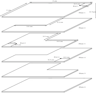
Figure 2-3: Illustrative example of multilayered PDN. (a) Original four layered structure (b) Original structure decomposed into two separate multilayered structures. ... 24

Figure 2-4: (a) Unit cell from the four layered PDN of Fig. 2-3. (b) Lumped π model of unit cell. ... 27

Figure 1-5: Three-dimensional and cross sectional views of an interconnect structure. ... 19

Figure 1-6: Lumped transmission line model for single transmission line. ... 21

Figure 1-7: Circuit realization of MoC for a two-conductor transmission line………..24

Figure 1-8: Circuit realization of DEPACT macromodel. ... 27

Figure 1-9: Longitudinal partitioning of single transmission line using lumped RLGC model ... 31

Figure 1-10: Subcircuits generated from Fig. 2.9 for single transmission line (no optimization) ... 31

xi

|Y12| (ε12(η))………41

Figure 3-3: Transient response of Example 1 using the proposed algorithm, HSPICE‟s W-element and direct IFFT. (a) Response at P2. (b) Response at P3. ... 41

Figure 3-4: Propagation delay capture of Example 1 using the proposed algorithm, HSPICE‟s W-element and direct IFFT. (a) Response at P2. (b) Response at P3. ... 44

Figure 3-5: Two port circuit for Example 2……….46

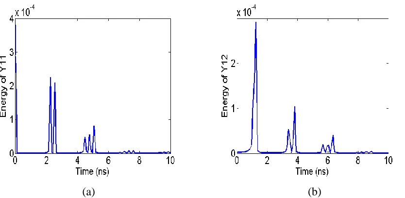
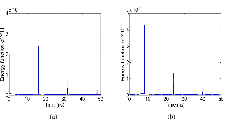
Figure 3-6: Evaluating delay peaksof Example 2. (a) Energy of |Y11| (ε11(η)) (b) Energy of |Y12| (ε12(η))………...………...47

Figure 3-7: Transient response at far end of Example 2. ... 49

Figure 3-8: Two port circuit for Example 3. ... 49

Figure 3-9: Transient response of Example 3 using the proposed algorithm, HSPICE‟s W-element and single delay extraction based IFFT [19]. (a) Response at Port 1. (b) Response at Port 2. ... 52

Figure 4-1: Lumped circuit of a single face of unit cell. ... 55

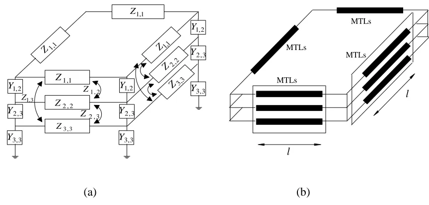
Figure 4-2: (a) Multilayered unit cell. (b) Unit cell model using MTLs. ... 58

Figure 4-3: DEPACT realization of the single face of the unit cells using MTLs. ... 59

xii

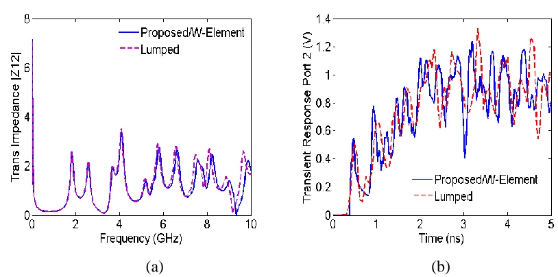
model. (a) Frequency domain response (Z12). (b) Transient response at Port 2. ... 63

Figure 4-6: 6 coupled multilayered PDN problem of Example 2………...65

Figure 4-7: Comparison of S parameters of Example 2 using the proposed and the lumped models for cell dimensions l = 0.5 cm. (a) Magnitude of S12. (b) Magnitude of S13. ... 67

Figure 4-8: Comparison of S parameters of Example 1 using the proposed model (l = 0.5 cm) and the lumped model (l = 0.167 cm). (a) Magnitude of S12. (b) Magnitude of S13... 67

Figure 4-9: Comparison of transient response of Example 2 using the proposed macromodel (l = 0.5 cm) and the lumped model (l = 0.167 cm) (a) Response at Port 2 (b) Response at Port 3... 68

Figure 5-1: SPICE equivalent circuit of a MTL using DEPACT………...73

Figure 5-2: Partitioning of MTLs into subcircuits for waveform relaxation………...75

Figure 5-3: Hybrid GS-GJ iterative technique. ... 78

Figure 5-4: Circuit of Example 1……….85

Figure 5-5: Transient response for Example 1. All line lengths are l = 30 cm. (a) Transient response at output port N1. (b) Transient response at output port N2………86

Figure 5-6: Convergence properties of the proposed hybrid iterative technique compared to GJ. All line lengths are l = 30 cm………86

xiii

Transient response at output port N1. (b) Transient response at output port N2…………...87

Figure 5-9: Scaling of computational cost for Example 2. (a) Scaling of computational cost

with line length (l) (b) Scaling of CPU speed up with number of CPUs (p) (l = 200 cm)...89

Figure 6-1: Geometry of a multiconductor transmission line exposed to an incident

field………..93

Figure 6-2: Discretization of MTL using DEPACT in the presence of incident

fields……….97

Figure 6-3: Proposed circuit representation of the incident field coupled with ith lossless

section. (a) Prior to grouping of the lumped sources. (b) After grouping of the lumped

sources using (6.20). ... 100

Figure 6-4: Three coupled microstrip lines of Example 1. (a) Geometry of the transmission

lines. (b) Circuit layout of the transmission lines………..102

Figure 6-5: Transient response for Example 1 using the proposed LP-WR algorithm and full

simulation. (a) Transient response at output port 4 (b) Transient response at output port 5.103

Figure 6-6: Transient response (Vout) of inverter in Example 1 with incident fields……….104

Figure 6-7: Computational efficiency of the proposed LP-WR algorithm over full EMI

simulation. (a) Scaling of computational cost with line length (l) (b) Scaling of CPU speed up

xiv

cell. (b) DEPACT representation of unit cell. (c) Equivalent circuit model of unit cell)…..111

Figure 7-2: Partitioning along the natural MoC interfaces provided by DEPACT model…112

Figure 7-3: Proposed 2D partitioning………113

Figure 7-4: PDN structure of Example 1………...120

Figure 7-5: Transient response for Example 2 using the proposed WR algorithm and full

simulation. (a) Transient response at output port B using decoupling capacitors. (b) Transient

response at output port B without decoupling capacitors...………..122

Figure 7-6: PDN structure of Example 1………...124

Figure 7-7: Scaling of computational cost for Example 2. (a) Scaling of computational cost

with number of subcircuits (N0) (number of CPUs set to 1). (b) Scaling of CPU speed up with

number of CPUs (p) (N0 = 100)……….125

xv

CAD Computer aided design

CMOS Complementary metal oxide semiconductor

DEPACT Delay extraction-based passive compact transmission-line macromodel

EMI Electromagnetic interference

IC Integrated circuit

IFFT Inverse fast Fourier transform

LP-WR Longitudinal partitioning based waveform relaxation

MNA Modified nodal analysis

MoC Method of characteristics

MRA Matrix rational approximation

MTL Multi-conductor transmission line

ODE Ordinary differential equation

PCB Printed circuit board

PDE Partial differential equation

PDN Power distribution network

PMoC Passive method of characteristics

PRIMA Passive reduced-order interconnect macromodeling algorithm.

p.u.l Per-unit-length.

SPICE Simulation program with integrated circuit emphasis

TEM Transverse electromagnetic

TP-WR Transverse partitioning based waveform relaxation

xvi

Chapter 1

1

Introduction

1.1

Background and Motivation

Computer aided design (CAD) has become an integral step in the design, analysis and testing

of very large scale integrated (VLSI) circuits and their packaging into electronic products.

Through CAD, it has now become possible to perform complex sensitivity analyses,

tolerance analyses and optimization studies of VLSI circuit design at the push of a button

leading to easier understanding of design roadblocks and performance tradeoffs. However,

for CAD to remain relevant, the simulations tools have to be able to take into account the

rapid growth in packaging density, operating speeds and diverse functionality of modern

integrated circuits (ICs).

A key aspect of CAD is signal integrity analysis. Signal integrity analysis is the investigation

of signal quality as it travels through high speed interconnects. At high frequencies of

operation, interconnects behave like distributed transmission lines. This distributed

distortion, attenuation, electromagnetic interference (EMI), ringing and crosstalk which can

severely degrade system performance and even lead to false switching of logic gates and

damage terminating electronic circuits [1]-[3].

Another critical area of CAD is power integrity analysis. Power integrity analysis is the study

of the distribution of the power supply to the active electronic circuits through power

distribution networks (PDNs) [4]-[5]. Like high speed interconnects, PDNs are distributed

networks and often are the sites of resonance, ground bounce, simultaneous switching noise

(SSN), electromagnetic radiation and return path discontinuities (RPDs). Such effects not

only lead to unreliable power distribution within the system but when coupled to the signal

network, can adversely affect the signal quality as well [5].

Based on the above discussion, it is noted that accurate modeling of interconnects and PDNs

are extremely important for the early stages of iterative electronic product design. However,

commercial circuit simulators with integrated circuit emphasis such as SPICE [6] are

typically unable to perform simulation of distributed networks terminated by nonlinear

circuits (typically complementary metal oxide semiconductor (CMOS) circuits) as they suffer

from the frequency/time mismatch problem. This frequency/time mismatch problem arises

from the fact that distributed networks are described by partial differential equations (PDE)

which are well represented in the frequency domain, whereas the transient responses of

nonlinear circuits are described in the time domain by nonlinear differential equations.

Hence, in order to perform transient analysis of distributed networks terminated by nonlinear

CMOS circuits, macromodeling algorithms are required to convert the governing PDEs into a

Macromodeling algorithms can be categorized into two classes – one class of algorithms deal

with modeling of networks where no knowledge of the physical characteristics of the

network structure is available whereas another class of algorithms deals with modeling of

networks where a priori knowledge of the physical characteristics of the network is available

and assuming a quasi transverse electromagnetic (TEM) mode of propagation through the

network.

For the case where no knowledge of the physical characteristics of the network exists, the

network is characterized by frequency domain, multiport tabulated data obtained either from

electromagnetic simulations or from measurements [7]-[21]. The behavior of high speed

distributed networks can be represented by frequency-dependent admittance, impedance, or

scattering parameters. It is noted that although an inverse fast Fourier transform (IFFT) can

be used to convert the multiport, frequency domain data into time domain for transient

analysis, since the tabulated data is bandlimited, direct IFFT cannot explicitly enforce the

delay of the port-to-port transfer functions and result in significant error in signal integrity

analysis [19]. In a recent work [19], a single delay extraction based IFFT macromodel was

developed. This algorithm was found to be highly accurate for networks with one dominant

delay. However, this technique was unable to capture higher order delays due to multiple

reflections at the far end of the network and hence has accuracy problems for general

distributed networks with multiple dominant delays in the transfer function [21].

Macromodeling algorithms of a network with known physical characteristics can be either

based on quasi-static lumped modeling algorithms or delay extraction based algorithms.

RLGC macromodel (for interconnect networks [1] and for PDNs [5]-[22]), PRIMA [23] and

matrix rational approximation (MRA) [24]-[25], to name a few. The advantage of these

algorithms is that they can be made to be passive by construction. However, lumped models

attempt to implicitly approximate the delay of distributed networks such as high speed

interconnects and PDNs as a rational function and hence require high order approximations

to accurately capture the high frequency poles contributed by the delay portion of the transfer

function. This leads to exorbitantly large models which are inefficient for use in the early

design cycles.

On the other hand, delay extraction based techniques explicitly extract the delay of the

network, thereby explicitly capturing most of the high frequency poles of the transfer

function. The remainder of the transfer function can be approximated using a low order

rational approximation leading to relatively compact and more accurate models than lumped

modeling techniques. The generalized method of characteristics (MoC) is one such algorithm

which has proved to be very efficient for long, low loss interconnect modeled as

multiconductor transmission lines (MTLs) [26]-[30]. However, a major limitation of MoC is

the potential loss of passivity that can occur in the model. Since transmission lines are

passive elements, loss of passivity of the macromodel can leads to unstable results in the

transient simulation even when terminated with passive circuits [8].

Recently, the delay extraction based passive macromodeling algorithm (DEPACT) has been

found to provide very good results for modeling long interconnects compared to lumped

models [31]-[32]. Not only does the DEPACT use a delay extraction feature for efficient

generalized MoC algorithm. Nonetheless, the DEPACT being a sectioning based model, its

accuracy depends on the losses of the interconnect network, line length and the maximum

frequency of operation. As these parameters increase, additional sections need to be added

thereby augmenting the computational costs of the algorithm. Thus, attempts to mitigate the

rapid increase in simulation cost of the DEPACT algorithm with the network size and

frequency of operation are still an open problems. Recently the delay extraction based

W-element model (based on the MoC and provided by the SPICE platform) has been utilized to

efficiently model single layered PDNs [33].

1.2

Objectives and Contributions

The objective of this thesis is to develop efficient broadband macromodeling algorithms for

distributed networks such as high speed interconnects and PDNs and the following

contribution are presented in this thesis.

Firstly, a delay extraction based IFFT algorithm is proposed for accurate and delay-causal

transient analysis of high speed interconnects characterized by their frequency domain,

multiport Y parameter data. The proposed algorithm uses time-frequency decompositions to

extract multiple propagation delays and the associated attenuation losses from the frequency

domain data in a piecewise manner, and then implements IFFT to efficiently convert the

frequency response into a sum of delayed time domain responses. Numerical examples

illustrate that the proposed algorithm shows significantly more accurate results for networks

Secondly, for PDNs where the physical characteristics of the structure are known and the

electrical model can be derived from the discretization of the Helmholtz wave equation,

novel delay extraction based modeling techniques have been developed. These techniques are

based on the extension of the one dimensional (1D) DEPACT algorithm to the single layered

(2D) and multilayered (3D) PDN structures in presence of holes, apertures and irregular

geometry. Numerical examples have been performed to demonstrate the efficiency and

accuracy advantages of the DEPACT algorithm for these 2D and 3D problems compared to

the existing lumped modeling techniques.

Thirdly, for the parallel simulation of electrically long interconnects, a longitudinal

partitioning based waveform relaxation (LP-WR) algorithm is developed. The key feature of

this WR algorithm is that it exploits the DEPACT algorithm to ensure weak coupling

between the subcircuits and consequently provides swift convergence. Furthermore, a hybrid

iterative technique that combines the high parallelizability of Gauss-Jacobi iterative

algorithms with the fast convergence of Gauss-Seidel iterative algorithms has been

developed for further accelerating the convergence of the WR iterations. The overall

algorithm exhibits good scaling with both the size of the network involved and the number of

CPUs available leading to significant improvement in the computational costs over

sequential SPICE algorithms.

Fourthly, electromagnetic interference (EMI) analysis of high speed interconnects using the

above LP-WR algorithm has been proposed as well. A key feature of this work is that the

problem where EMI analysis is required. Hence, the proposed parallelizable algorithm is

significantly more efficient than sequential SPICE algorithms for EMI.

Finally, the proposed WR algorithm has been extended to the problem of efficient modeling

of singly layered (2D) PDNs. For PDN problems, the longitudinal partitioning algorithm and

the hybrid WR iterations have been extended to a 2D partitioning scheme compatible with a

2D hybrid WR iterations. The overall algorithm retains its highly parallelizable and exhibits

good scaling with both the size of the PDN involved and the number of CPUs available,

similar to what has been observed for interconnect problems.

1.3

Organization of the Thesis

The thesis is organized as follows. Chapter 2 reviews the existing state of art for

macromodeling of high speed interconnects and PDNs. This chapter covers both classes of

macromodeling techniques – those based on port-to-port tabulated data as well as those based

on quasi-TEM mode of propagation where the physical structure of the network is known.

Moreover, a review of existing longitudinal partitioning based WR algorithms is also

provided. Chapter 3 deals with the development of the proposed delay extraction based IFFT

algorithm for macromodeling of interconnects characterized by port-to-port tabulated data.

Examples are provided to compare the proposed work with pure IFFT based techniques and

single delay extraction based IFFT techniques. Chapter 4 deals with the development of the

delay extraction based macromodeling techniques for single layered (2D) and multilayered

accuracy of the proposed algorithms with respect to existing lumped techniques. Chapter 5

covers the proposed LP-WR algorithm for high speed interconnects and provides examples to

demonstrate the advantages of this WR technique over sequential algorithms and other

existing longitudinal partitioning based WR algorithms. Chapter 6 extends the LP-WR

algorithm of Chapter 5 to the problem of EMI in high speed interconnects and chapter 7

covers the extension of the proposed WR algorithm to the 2D problem of PDNs. Finally,

Chapter 8 summarizes the proposed work and also presents some suggestions for future

Chapter 2

2

Background and Literature Review

2.1

Introduction

Interconnects provide the physical path for the signal to propagate between electrical

devices in chips, electrical packages, printed circuit boards (PCB) etc. At low

frequencies, interconnects can be modeled using a quasi-static lumped electrical RLGC

model [1]-[2]. However, at high frequencies, when the wavelength of the travelling

electromagnetic wave surrounding the conductors are much smaller than the line length,

interconnects behave as distributed transmission lines and this distributed nature of

performance is responsible for non ideal effects such as signal delay, distortion,

attenuation, ringing and crosstalk [1], [2]. Similarly, PDNs at low frequencies behave as

purely capacitive elements while at high frequencies they too exhibit distributed behavior

[5]. In course of this chapter, the state of the art regarding macromodeling of such high

speed distributed networks will be reviewed. The organization of this chapter is as

follows: Section 2.2 explains macromodeling of high speed interconnect networks which

the modeling of PDN structures using the conventional lumped electrical RLGC model.

Section 2.4 explains macromodeling of high speed interconnect networks derived from

quasi-TEM mode of propagation and Section 2.5 provides several transmission line

macromodels for nonlinear circuit simulators. Finally, Section 2.6 describes existing WR

techniques for parallel simulation of large networks.

2.2

Macromodeling based on Measured Data

Typically large interconnect networks can be characterized by their frequency domain,

multiport admittance (Y), impedance (Z), or scattering (S) parameters obtained as tabulated data [7]-[21]. The goal of macromodeling is to derive accurate models based on

this tabulated data which can then be reused for any arbitrary terminations.

Presently, there are two approaches towards deriving macromodels of interconnect

networks characterized by band limited frequency domain data. One approach is based on

approximating the tabulated data using rational functions via least squares curve fitting

techniques such as vector fitting (VF) [10] and interpolation-based complex rational

approximation [7]-[8]. In the time domain, the rational macromodel can be analytically

represented as a sum of decaying exponentials and convoluted with any input signal

using the recursive convolution technique [34]. The drawback of such rational

macromodeling techniques lie in the fact that they attempt to implicitly capture the delay

feature of the transfer function using rational basis functions and consequently require a

large number of rational functions for broadband macromodels. Since the memory and

respectively, where Np is the number of identified poles, for conventional rational

modeling of interconnect networks, Np may be exorbitantly large and such models are

computationally expensive to obtain [19]. Furthermore, passivity constraints need to be

satisfied by the derived rational models in order to guarantee stable responses for the

model connected to any arbitrary terminations [8]. Typical passivity enforcement

techniques, such as that reported in [35], result in additional post processing and may

increase the incurred computational costs.

Recently, new curve fitting techniques have been proposed based on delayed rational

macromodeling techniques [17]-[18]. These techniques extract the propagation delays

from the tabulated data while the remaining attenuation losses of the frequency response

are approximated using rational curve fitting. This allows the time domain transfer

function to be obtained as a sum of delayed exponentials which can be convoluted with

any given input using the recursive convolution technique [34]. While such models are

more compact in nature, they still require additional passivity enforcement schemes

before they can be integrated with any arbitrary circuit termination.

An alternative approach seeks to simply perform an IFFT operation to convert the

tabulated frequency domain data into time domain data, which can then be convoluted

with any input using a numerical convolution technique. The advantages of an IFFT

operation lies in the fact that it does not require a least square fitting operation and hence

avoids the large memory and time constraints of such techniques. Moreover, an IFFT

operation does not require any passivity enforcement. However, these techniques are not

delay-causal by construction which is defined as an impulse response equal to zero for t <

band limited data does not explicitly preserve the delay of the transfer function and leads

to signal fluctuations in early time [21]. In order to preserve the delay causality of the

model, a single delay extraction based IFFT algorithm was proposed in [19] and is

reviewed below.

Let us consider an interconnect network characterized by its frequency domain, multiport

Y parameter data as

) ,.., 1 , ( )]; ( [ )

(s  Y_ij s i j P

Y (2.1)

where

sTij

ij

ij s H s e

Y ( ) ( )  (2.2)

and Hij represents the remainder of the transfer function once the dominant delay Tijhas

been extracted. From (2.1), it is noted that

| ) ( | | ) (

|Y_ij s  H_ij s (2.3)

Based on (2.3), arg(Hij) can be obtained from the Hilbert transform as

   

  







 

d j

j s j

Y s

H_{ij ij} )

2 cot( | ) ( | ln 2

1 )) (

arg( _(2.4)

where ρ is the Cauchy's principal value of the integral and arg(x) is the argument of x

[19]. Based on the knowledge of (2.3)-(2.4), the dominant delay Tij can be approximated

    

  

    

   



) (

) ( arg

s H

s Y slope

avg T

ij ij

ij (2.5)

where avg(x) represents the average of a tabulated data x. Once the delay Tij has been

extracted, performing the IFFT on Hij and enforcing the extracted delay yields a

delay-causal response. Due to the explicit delay enforcement feature of this algorithm, it

provides more accurate transient results compared to directly implementing IFFT on the

data.

It is noted, however that for the Hilbert transform of (2.4), Hij has to be a minimum phase

response (i.e. it does not have any poles or zeros in the right half of the Laplace plane)

[36]. This is true if there are no higher order delays embedded in Hij or if the higher order

delays have very little contribution to the function Hij. This is because any general delay

terms ( sT

e ) embedded in Hij may contribute zeroes in the right half of the Laplace plane.

However, multiple reflections of the signal at the terminations of interconnect networks

may result in significantly large higher order delays. As a result, sophisticated algorithms

to extract the higher order delays are required for the case when Hij may not exactly be a

minimum phase response.

2.3

Macromodeling of Power Distribution Networks

Power Distribution Networks (PDNs) provide a path for the power supply to the core

logic circuits and I/O drivers of high speed digital systems [4]-[5]. Ideally PDN should

currents induced by the simultaneous switching of digital circuits do not lead to excessive

noise propagation over the PDN [4]-[5]. However with the progressive increase in clock

speed, scaling of supply voltage, high switching speed of logic circuits and reduced noise

margins, effects like ground bounce, EM interference and SSN noise arising in the PDNs

can quickly lead to undesirable voltage fluctuations and propagation delays in chip, board

and packaging levels. Hence PDNs are fast emerging as a critical area for

electromagnetic compatibility (EMC) and power integrity (PI) verification for high speed a

Dielectric

d

t

Unit cell a

Dielectric

b

d

t

1 2 Nc+1

Nr+1

2

Nc

Nr

(a) (b)

Figure 2-1: Modeling of PDN. (a) Single layered PDN. (b) Discretization of PDN into

unit cells.

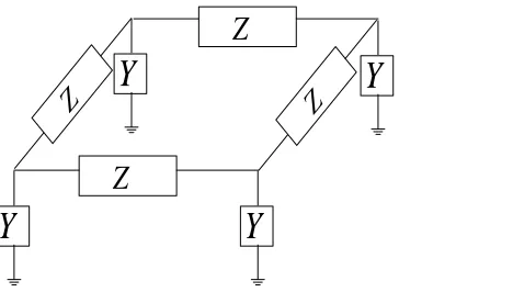
Z

Z

Y

Y

Y

Z

Y

Z

Figure 2-2: π representation of a unit cell. Each Z and Y block can be modeled using

packages.

2.3.1

Single Layered PDNs

A PDN consisting of a rectangular signal/ground plane with single layered dielectric in

between and assumed to be free of any surface irregularity is considered in Fig. 2-1(a).

This PDN is typically represented in the frequency domain by the Helmholtz PDE [5]. In

order to derive a macromodel that can represent the electrical performance of the PDN,

typically finite difference discretization of the Helmholtz PDE is performed. Such a

discretization of the PDE can be physically visualized as the discretization of the

geometry into a grid of unit cells as shown in Fig. 2-1(b). The equivalent circuit

representing a unit cell can be obtained from the physical and electrical parameters of the

plane using a quasi-static model provided the dielectric separation between the power and

ground plane pairs is much smaller compared to the dimensions of the plane [5].

Considering a square unit cell of dimensions (l) with a dielectric separation of (d)

between planes, thickness of metal (t), metal conductivity (ζ), loss tangent () and

relative permittivity (r), the equivalent electrical parameters are

  



 

 

0 2

2 ), tan(

, ,

, 2

s R

C G

d L d l C

t R

s

o r

o

 

 



(2.6)

where s =2jπf is the Laplace variable, f is the instantaneous frequency, ε0 and µ0are the

permittivity and the permeability of free space, εr is the relative permittivity of the

dielectric and R, L, G, C and Rs are the resistive, inductive, capacitive, conductive and

skin effect losses contribution of the unit cell respectively [5]. Based on the parameters of

[5]. In particular, the Z and Y blocks of the π model can be realized using RL and RC

ladder networks respectively as explained in [5] thereby allowing for their SPICE

implementation.

2.3.2

Multilayered PDNs

Realistic multilayered PDN designs consist of multiple irregular shaped planes stacked

vertically. Due to the presence of apertures, holes and irregular geometry of the planes,

wraparound currents are supported on the plane layers which lead to the electromagnetic

(EM) coupling between individual planes in the transverse direction [5], [37].

For multilayered PDNs, modeling techniques based on the multilayered finite difference

method (MFDM) has been proposed [37]. This MFDM model discretizes the

multilayered PDN structure to yield an equivalent three dimensional (3D) lumped circuit

model which can be directly realized in SPICE for both frequency and transient analysis.

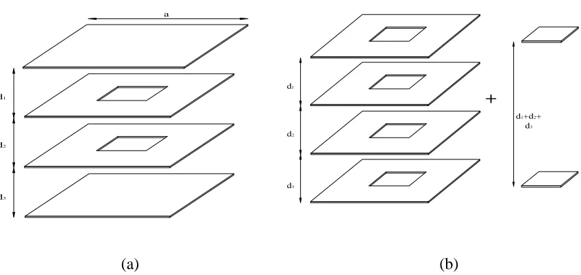
In order to understand how that is possible, the illustrative example consisting of four

d1

d2

d3

a

d1

d2

d3

d1+d2+

d3

+

(a) (b)

Figure 2-3: Illustrative example of multilayered PDN. (a) Original four layered structure

vertically stacked square planes as shown in Fig. 2-3(a) is considered. It is observed that

the presence of an aperture in the middle planes will give rise to wraparound currents

thereby leading to EM coupling between all four planes. The coupled four plane structure

can be considered as made up of two separate multilayered PDN structure consisting of

four and two layers as shown in Fig. 3(b). For any multilayered structures of Fig.

2-3(b), each ith plane assigns the i+1th plane below it as its local reference plane. In other

words, considering a current on the bottom of the ith plane, the return path for the same

current is considered to exist on the top of the i+1th plane below.

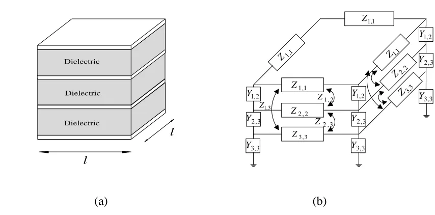
A common methodology of modeling the multilayered PDNs of Fig. 2-3(b) is by

discretizing the structures into numerous multilayered unit cells based on a finite

difference treatment of the Helmholtz equation [37]. A unit cell of the four layered PDN

section of Fig. 2-3(b) is shown in Fig. 2-4(a). The resistive (Ri), inductive (Li), capacitive

(Ci), conductive (Gi) and skin effect loss (Rˆi) parameters of each i th

plane of the unit cell

Dielectric

l

l

Dielectric Dielectric

2 , 1

Y Z1,1

2 , 2

Z

3 , 3

Z

1 , 1

Z

2 , 2

Z

3 , 3

Z

1 , 1

Z

1 , 1

Z

3 , 2

Y

3 , 3

Y

2 , 1

Y

3 , 2

Y

3 , 3

Y

2 , 1

Y

3 , 2

Y

3 , 3

Y

2 , 1

Z

3 , 2

Z

3 , 1

Z

(a) (b)

Figure 2-4: (a) Unit cell from the four layered PDN of Figure 2-3. (b) Lumped π model

of Fig. 2-3(a) with respect to its local reference (i+1th plane of the unit cell of Fig. 2-4(a))

can be described using a quasi-static model provided the dielectric separation between the

planes is much smaller compared to the dimensions of the plane similar to what has

already been done in (2.6) [5]. In order to obtain an equivalent circuit model of Fig.

2-4(a) compatible with SPICE, the local reference planes of Fig. 2-2-4(a) are replaced by a

single common ground plane which is taken as the bottommost planes in the stacked

structures. As a result, the electrical parameters of each ith plane of the unit cell of Fig.

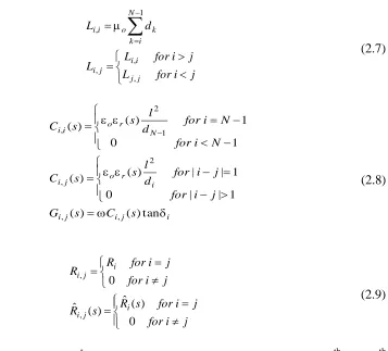
2-4(a) with respect to the common ground is obtained as [5], [37]

       



where Li,j,Ci,j,Gi,j,Ri,j and Rˆi,j represent the coupling term between the i

th

and jth

plane for 1i,jN1 and N represents the total number of PDN layers (i.e. N = 4 for

Fig. 2-4). It is noted that (2.7) represent the transverse coupling due to the magnetic flux

Overall, (2.7)-(2.9) provides a generalized quantification of the coupling of any general N

layered PDN. Based on (2.7)-(2.9), the equivalent lumped π-model representing each unit

cell is illustrated in Fig. 2-4(b) [37] where each of the Z and Y blocks of Fig. 2-4(b) is

realized in SPICE using a lumped RL and RC network respectively [5].

For the accurate modeling of the distributed nature of PDNs, the geometric dimensions of

each unit cells of Fig. 2-1(b) (single layered PDNs) and Fig. 2.4(a) (multilayered PDNs)

has to be very small compared to the PDN dimensions. This leads to very large modified

nodal analysis (MNA) matrices representing the PDN when realized using commercial

circuit simulators like SPICE. Furthermore, realization of the frequency dependent

parameters of (2.7)-(2.9) using lumped RL/RC ladder networks as proposed in [5], [37]

will lead to introduction of additional nodes and further augmentation of the MNA

matrices. Thus, computational costs of modeling PDNs are typically expensive and

alternative methodologies for efficient modeling of PDNs are still being investigated.

Ground plane ε, μ0

Interconnect

Substrate

Interconnect

Substrate

2.4

High Speed Interconnect Modeling

Figure 2-5 shows the physical structure of a typical interconnect network. The

complexity of the interconnect macromodel depends on the physical dimensions and

operating frequency of the circuit. For cases where the minimum wavelength of the

travelling electromagnetic wave through the medium is comparable with the cross

sectional dimensions of the interconnect network, full wave models are required. On the

other hand, as long as the minimum wavelength of the travelling electromagnetic wave is

much larger than the cross sectional dimensions of the interconnect network, a TEM

mode of propagation is the dominant mode of wave propagation. In TEM mode of

propagation, the electric and magnetic fields surrounding the space around the line

conductors are transverse or perpendicular to the line axis and to each other [1]. TEM

mode exists for transmission lines with homogenous medium and perfect conductors. In

inhomogeneous mediums, electromagnetic waves are generated with different velocities.

Moreover, interconnect networks with imperfect conductors produce electric fields along

the surface conductor. Such interconnect structures violate the TEM wave characteristics,

since TEM waves propagate with only one velocity and have no electric field along the

surface conductor. However, for many lossy interconnects in presence of inhomogeneous

medium, the results are almost similar to TEM structures and thus they can be

approximated as TEM mode, referred as quasi-TEM assumptions. One of the important

characteristics of TEM mode of propagation (which is approximated for non-perfect

conductors in quasi-TEM modes) is the ability of expressing the voltage and current

   

     

 



 

   

  



) , (

) , ( )

, (

) , (

s x

s x (s))

s (s) (

(s)) s (s) ( s

x s x

x I

V 0

C G

-L R

-0

I V

(2.10)

where x is the position variable along the axis of the conductors; V(x, s) and I(x, s) represent the spatial distribution of voltage and current vectors of the multi-conductor

transmission lines (MTLs) respectively; R(s), L(s), G(s) and C(s) are the frequency dependent per unit length (p.u.l.) resistance, inductance, conductance and capacitance

matrices, respectively. The p.u.l. parameter matrices can be determined by a can be

obtained from a static solution of the Laplace equation in the 2-D plane containing the

cross section of the conductors of Fig. 2-5 [1]. The difficulty with modeling of

interconnects using (2.10) is that they cannot be directly linked to circuit simulators such

as SPICE. This is because typical circuit simulators solve nonlinear ordinary differential

equations (ODEs) while Telegrapher‟s equations are expressed as PDEs. To overcome

this difficulty, numerical techniques are used to convert distributed models into ODEs as

explained in detail in the next subsection.

RΔx LΔx

CΔx GΔz

ground

x=0 x x+Δx x=l

i(0,t) i(l,t)

v(0,t) v(l,t)

i(x+Δx,t) i(x,t)

z _x+Δx

v(x,t) v(x+Δx,t)

2.5

Simulating Interconnects in SPICE-like Simulators

For the case when the physical characteristics of the interconnect structure is known and

quasi-TEM is assumed, the electrical performance of interconnects can be expressed

using the Telegrapher's partial differential equations (PDE). Commercial circuit

simulators like SPICE being unable to solve the PDE's in the time domain,

macromodeling algorithms are required to convert the PDE to ordinary differential

equations (ODE) which can be solved by numerical integration. Moreover,

macromodeling algorithms can also be extended to perform EMI analysis due to incident

field coupling to lossy transmission lines. The following sections describe some of the

existing macromodeling techniques based on quasi-TEM mode of propagation, followed

by a review of incident field analysis.

2.5.1

Lumped Segmentation

Lumped segmentation technique uses lumped equivalent circuits of the transmission lines

to approximate Telegrapher‟s equations. Applying Euler‟s method [1] to (2.10) yields

   

     

 



 

    

 

  

  

) , (

) , ( )

, ( ) , (

) , ( ) , (

s x

s x

(s)) s (s) (

(s)) s (s) ( x

s x x s x

s x s x x

I V

0 C

G

-L R

-0

I I

V V

(2.11)

where x=[1,2,...,η ], Δx=l/η, η is the number of sections and l is the length of

interconnect. Equation (2.11) can be implemented by lumped equivalent circuit

composed of resistors, inductors and capacitors as shown in Fig. 2-6. In order to ensure

that the discretization of (2.11) is accurate, the value of Δx has to be very small. The

basic rule of thumb to determine the value of Δx is to ensure that the number of segments

r t

LC l

n20  _(2.12)

where t_r is the rise/fall time. The lumped segmentation model is passive and provides a

direct method to discretize (2.10). However as the rise time of signal shortens with VLSI

technology and/or if the interconnect is electrically long, many lumped elements are

required for an accurate model. This leads to large MNA matrices thereby increasing the

simulation time.

2.5.2

Matrix Rational Approximation

Matrix rational approximation (MRA) macromodel directly converts the Telegrapher‟s

equations into time domain macromodels based on analytic rational approximations of

exponential matrices [24]-[25]. An important feature of the MRA macromodel is that it is

passive by construction. To describe this macromodeling algorithm, the solution of (2.10)

can be written in the Laplace-domain as an exponential matrix function as

   

        

) (0

) (0 )

( ) (

s ,

s , e

s l,

s l,

I V I

V _Z









s s

s s

    

 

 

 



0 C

G

L R

0 Z

) ( s ) (

) ( s ) (

(2.13)

where l is the length of the transmission line. The exponential matrix eZ in (2.13) can be

expressed with a matrix rational approximation as

) ( )

(Z Q Z

where P_M(Z) and Q_N(Z) are polynomial matrices







 

 

 M

i

i M

i

i i M

i M i M

M i M p

0

0 (2 )!!( )!

! )! 2

( )

(Z Z Z

P







 

 

 N

i

i N

i i i N

i N i N

N i N q

0

0 (2 )!!( )!

! )! 2 ( )

(Z Z Z

Q (2.15)

After some mathematical manipulations, the results of (2.15) can be used to obtain a

macromodel represented by a set of ordinary differential equations, in a closed form

manner [24]-[25]. Since the MRA macromodel is described in terms of predetermined

coefficients p_i and q_i, and the p.u.l parameters, the macromodel can be constructed very

quickly. While the MRA macromodel has been proved to be highly efficient for

interconnects with small line length, it is not very computationally efficient for

electrically long lines since the delay of the transmission line is not extracted. Hence, for

long lines, a higher order of approximation is required to express eZ as a matrix rational

approximation. In the following subsections two common delay extraction macromodels

are reviewed that addresses the computational constraint of such lumped model. Figure 2-7: Circuit realization of MoC for a two-conductor transmission line.

+

-+

-0

Z

1

v

1

i

2

v

i

1

w

2

w

0

Z

+ +

-2.5.3

Method of Characteristics

Among the most commonly used algorithms are those based on the generalized method

of characteristics (MoC). The MoC extracts the line-propagation delay and produce exact

models when applied to lossless transmission lines [26]. Over the years, these algorithms

have been extended to model lossy MTLs [27]-[30]. The efficiency of MoC is derived by

extracting the propagation delay which allows the attenuation function to be

approximated with a low-order rational function. This significantly reduces the

computational complexity of the transfer function; especially for long lines with low

losses.

The original method of characteristics [26] is able to represent interconnects as ODEs

containing time delays. Although the original method of characteristics was developed in

the time-domain using what is referred as characteristic curves (hence the name), a

simpler alternative derivation in the frequency-domain is presented. The frequency

domain solution of (2.13) for a two-conductor transmission line is

           

  

 

 

 

     

 

 



2 1 2

2

2 0

2 1

1 2

2 1

) 1

( 1

V V

e e

e e

e Z I

I

l l

l l

l  

 















 



Z₀   /  (2.16)

where  is the propagation constant and Z₀ is the characteristic impedance. After some

2 2 0 2 1 1 0 1 ; W I Z V W I Z V     (2.17)

where W₁ and W₂ are defined as recursive relations

] 2 [ ]; 2 [ 1 1 2 2 2 1 W V e W W V e W l l         (2.18)

For lossless transmission lines,  and Z₀can be reduced to

LC s 

 ; Z₀  L/C (2.19)

which makes γ a purely imaginary number and Z0 a real constant. The time domain

solution of MoC can be obtained by taking the inverse Laplace transform of (2.17) and

(2.18) as ) ( ) ( 2 ) ( ); ( ) ( 2 ) ( ); ( ) ( ) ( ); ( ) ( ) ( 1 1 2 2 2 1 2 2 0 2 1 1 0 1









where τ = γl is represented as a delay term. An equivalent circuit realization of time

domain macromodel of a lossless transmission line is demonstrated in Figure 2-7. For the

case of lossy transmission lines, γ is not purely imaginary and Z0 is not a real constant

and therefore, the direct time domain representation is not possible. In this case,

numerical techniques have been proposed to incorporate lossy transmission line models

2.5.4

Delay Extraction-Based Passive Compact Transmission-Line

Macromodeling Algorithm (DEPACT)

Another delay extraction based algorithm is the DEPACT macromodel which, unlike the

MoC can be made passive by construction [31]-[32]. To better understand the DEPACT

macromodel, the Z matrix of (2.13) is rewritten as

B A

Z s (2.21a)

l

-    

  

 





0 )

(s) s( (s)

) (s) s( (s) 0

C C G

L L R

A ; _l

  

  

 





0 0

C

L

B (2.21b)

and L_ L()and C_ C() are the extracted p.u.l inductance and capacitance of the line and l represents the line length.

n

e 2 (s)

A

n

e

) (

B

Lossy # 1 Lossless # 1 Lossy # 2 Lossless # 2 Lossless # n Lossy # n+1

0

Z

Lumped Circuit Elements

……...

1

W

Lossy # 1 Lossless - MoC # 1 Lossy # 2 Lossless - MoC # 2 Lossless - MoC # n Lossy # n+1

single transmission line

2

W

n e

(s)

A _……...

n

e

) B(

Lumped Circuit Elements

Lumped Circuit Elements 0

Z Z0 W3 W4 Z0 Z0 W2n1 W2nZ0

n

e 2 (s)

A

n

e

) (

B

The basic idea of the delay extraction-based passive compact transmission-line

(DEPACT) macromodeling algorithm is to separate the extracted delay terms ( sB

e ) from

) (A sB

e  thereby enabling eA to be modeled using a low order rational function. However,

this is not a trivial task since the matrices A and sB do not commute, (i.e. A sB A sB

e e e(  )  ).

To approximate (AsB)

e in terms of a product of exponentials, a modified Lie product

[38] is used as





 _ n _

i

n i e

1  Ψ

sB

A _(2.22a)

n n

s n

i e2 e e2

A B A



Ψ (2.22b)

where n is the number of sections. The associated error of the approximation scale to the

second power of number of sections n, as ||



converges to the exponential matrix of (2.13) with increase of number of sections n).

Equation (2.22) shows that the exponential function of (2.13) can be divided into

subsections of eA2n and esBn. The matrix eA2n represents a lossy line segment and

n s

e B represents a lossless line segment and the product of the two can be viewed as a

cascade of transmission line subnetworks [31], [32]. For a two-conductor transmission

line example, each Ψ_i in (2.22) can be realized as shown in Figure 2-8. Here, the lossy

terms can be macromodeled using the MRA algorithm (section 2.5.2) and the lossless

sections can be modeled using the MoC approach (section 2.5.3). The resulting

macromodels are of significant lower orders since for electrically long lines a significant

portion of the delay is already extracted using MoC [31]. It is however noted that the