Exploring the Association between Network, Cognitive, Structural Social Capital and the Risk of Clinical Depression in Taiwan

University of South Carolina

Scholar Commons

Theses and Dissertations

12-15-2014

Numerical Modeling of Free Surface Flows Using

Depth Averaged and 3D Models

Khaled Mamdouh Mohamed Abdo

Follow this and additional works at:https://scholarcommons.sc.edu/etd Part of theCivil and Environmental Engineering Commons

This Open Access Dissertation is brought to you by Scholar Commons. It has been accepted for inclusion in Theses and Dissertations by an authorized administrator of Scholar Commons. For more information, please [email protected].

Recommended Citation

Numerical Modeling of Free Surface Flows using depth averaged and 3D models

by

Khaled Mamdouh Mohamed Abdo

Bachelor of Science Cairo University, 2002

Master of Science Cairo University, 2008

Submitted in Partial Fulfillment of the Requirements for the Degree of Doctor of Philosophy in

Civil and Environmental Engineering College of Engineering and Computing

University of South Carolina 2014

Accepted by:

Jasim Imran, Major Professor M. Hanif Chaudhry, Committee Member

Enrica Viparelli, Committee Member Alessandro Cantelli, Committee Member

c

Dedication

Acknowledgments

I would like to express my sincere gratitude to my dissertation advisor, Professor Jasim Imran, for his support and guidance throughout my doctoral study in the University of South Carolina on the scientific and personal level. His steady influences, and patience were always there during all the times of difficulties. I would also like to thank the distinguished members of my dissertation committee: Prof. M. Hanif Chaudhry, Dr. Enrica Viparelli, and Dr. Alessandro Cantelli.

In addition, a deep thanks to my mentor and supervisor during my internship at Shell Technology Center, John M. Martin and Ru Smith. Their valuable advise and help during my internship were a major reason for me to have a successful and enjoyable internship.

Great thanks to my friends in the water resources group, and special thanks to Hesham Ezz and Mohamed El-Kholy who helped me a lot during the start of my Ph.D. journey. Also a very warm thanks to Hassan Ismail for his help specially during the last few weeks of my Ph.D..

There is no words that can describe my thanks and appreciation to all what my parents in Egypt did for me. They tought me how to love my work, how to be always eager to learn and were always helping and encouraging me throughout my whole life. Also I would love to express my thanks to my beloved wife, Reham Khedr, who always has faith in me and supported me during all our life together.

Finally, there is nothing of all of this that could be done without the help of my God. All thanks are due to Allah.

Abstract

The objectives of the research presented in this dissertation are to develop and apply numerical models to study free surface flows under different boundary conditions, bedform geometry and channel configuration. A 2D depth-averaged model is de-veloped by solving the Saint Venant or the shallow water equations using a finite volume method. An existing 3D model, developed in-house, that solves the Reynolds-averaged Navier-Stokes equations and conservation equations for suspended sediment and conservative species is adapted for free surface flows by solving the volume of fluid (VOF) equation using a compressive interface capturing scheme for arbitrary meshes, CICSAM. The depth-averaged or shallow water and the free-surface capturing 3D model are verified against experimental data on dam-break flow over a sloping bed.

un-derpredicts the wave trough amplitudes. The limitation of the present 3D model in capturing sharp changes in water depth is likely associated with the diffusive nature of 2-equation isotropic turbulence models.

The effects of freshwater discharge, dune amplitude and tidal amplitude on mixing between freshwater flow and an intruding salt wedge are studied using a 3D numerical model. Model results reveal intense mixing over bedforms, generation of large internal waves with salt concentration reaching the water surface and competing effects of freshwater discharge and the tidal amplitude. During the ebb tide, the freshwater discharge is able to push the salt wedge near or outside of the ocean side boundary. Four different types of disturbances over the dune field that are consistent with the field measurements are recognized.

Table of Contents

Dedication . . . iii

Acknowledgments . . . iv

Abstract . . . v

List of Tables . . . xii

List of Figures . . . xiii

Chapter 1 Introduction . . . 1

1.1 Free surface modeling . . . 1

1.2 Open channel flow through transitions . . . 1

1.3 Mixing over bedform under low and high tide conditions . . . 2

1.4 Point bar Fine Deposits: Controls, Process and Pattern . . . 3

1.5 Motivations and objectives . . . 3

1.6 Organization of the Proposal . . . 4

Chapter 2 Literature review . . . 8

2.1 Open channel flow through transitions . . . 8

2.3 Point bar fine deposits: controls, process and pattern . . . 11

Chapter 3 3D Numerical model . . . 19

3.1 Governing equations . . . 19

3.2 Boundary conditions . . . 21

3.3 Solution procedure . . . 22

3.4 Volume of fluid equation . . . 23

3.5 Model verification . . . 28

Chapter 4 Depth-averaged model . . . 31

4.1 Governing equations . . . 31

4.2 Numerical method and solution procedure . . . 32

4.3 Boundary conditions . . . 38

4.4 Model verification . . . 39

Chapter 5 Experimental setup and procedure . . . 42

5.1 Experimental setup . . . 42

5.2 Instrumentation . . . 42

Chapter 6 Experimental and numerical modeling flow in open channel contraction . . . 45

6.1 Model Application . . . 45

6.2 Comparison between Ippen-Dawson data and shallow water model results . . . 47

6.3 New measurement results . . . 48

6.5 Effects of flowrate: supercritical and subcritical flow . . . 50

6.6 SUMMARY . . . 51

Chapter 7 Numerical modeling of mixing over bedforms un-der low and high tide conditions using the volume of fluid method . . . 61

7.1 Scaling and Model inputs . . . 61

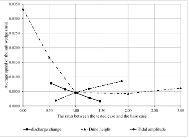
7.2 Effect of fresh water discharge variation . . . 62

7.3 Effects of dune height variation . . . 65

7.4 Effect of tidal amplitude variation . . . 66

7.5 Salt wedge speed and shear velocity . . . 67

7.6 Mixing over dunes . . . 68

7.7 Type of disturbance over the dunes . . . 69

7.8 Summary . . . 72

Chapter 8 Point bar Fine Deposits: Controls, Process and Pattern . . . 94

8.1 Point bar fine deposits controls . . . 94

8.2 Effect of river cross section . . . 96

8.3 Effect of planform shape . . . 97

8.4 Effect of sediment grain size . . . 99

8.5 Effect of flow discharge . . . 99

8.6 Effect of average bed slope . . . 100

8.7 Summary . . . 101

List of Tables

Table 7.1 Model input and initial boundary conditions . . . 73

List of Figures

Figure 1.1 Type of estuaries based on water circulation. A) salt wedge estuaries; B) partially mixed estuaries; C) well mixed estuaries;

D) fjord type estuaries. . . 6

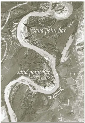
Figure 1.2 Cut bank erosion and point bar deposition as seen on the

Pow-der River in Montana (Moody et al., 2003). . . 7

Figure 2.1 Plan view for the contraction experiment, all the dimensions

are in meters . . . 14

Figure 2.2 Flow depth along the contraction center line. . . 14

Figure 2.3 Flow depth along the contraction wall. . . 15

Figure 2.4 Location of the field measurements by Kostaschuk et al. (2010)

in Fraser River estuary. . . 15

Figure 2.5 Field measurements by Kostaschuk et al. (2010) in Fraser River estuary; A) salt wedge propagation, B) u velocity, and c) v

velocity over the flat part of the river bed. . . 16

Figure 2.6 Field measurements by Kostaschuk et al. (2010) in Fraser River estuary; A) salt wedge propagation, B) u velocity, and c) v

velocity over the dune field of the river bed. . . 17

Figure 2.7 Ancient point bar deposits of the McMurray Formation,

Al-berta, Canada (Hubbard et al., 2011). . . 18

Figure 3.1 Schematic of free surface computation methods; A) surface methods where the surface is tracked explicitly either by using marker points or by attaching the surface to the grid B) Vol-ume methods where the fluid on either side of the surface are indicated by either massless particles or an indicator function

Ubbink (1997) . . . 29

Figure 3.3 Comparison between 3D model results and Larocque et al. (2012)

experimental measurements . . . 30

Figure 4.1 Comparison between SWE model results and experimental

mea-surements of Larocque et al. (2012) using Min-Mod flux limiter . 40

Figure 4.2 Comparison between SWE model results and experimental

mea-surements of Larocque et al. (2012) using Superbee flux limiter . 41

Figure 5.1 A) Plan view and B) longitudinal section for the contraction

experiment, dimensions are in meters . . . 43

Figure 5.2 Experimental setup; the picture includes the flume, gate, the portable cart, the sensor was used for measuring the water el-evations, and the flow meter used to monitor the flow rate at

the bottom right corner . . . 43

Figure 5.3 UNAM 18U6903/S14 - Ultrasonic distance measuring sensor. . . 44

Figure 6.1 A) plan view and B) longitudinal section for the 3D model grid . 53

Figure 6.2 Contour map for the flow depth using SWE-solver. The results are based on using A) Roe scheme (Roe, 1981) to solve the equa-tions, B) Roe(Roe, 1981) scheme with MUSCL scheme(Van Leer, 1979) and using Min-Mod flux limiter(Roe, 1985), and C) Roe(Roe, 1981) scheme with MUSCL scheme(Van Leer, 1979) and using

SUPERBEE flux limiter(Roe, 1985) . . . 54

Figure 6.3 Flow depths Contour map using the 3d−modelfor A) Q=0.041

m3/s, B) Q=0.050 m3/s, and C) Q=0.031 m3/s . . . 55

Figure 6.4 Comparison of measured and simulated water depth A) along

the centerline and B) near the wall . . . 56

Figure 6.5 Contour map of the flow depth for Q=0.041 m3_{/s. . . . 57}

Figure 6.6 The effect of changing the flow rate on the centerline measure-ments. The flow turned to subcritical flow in the case with

Figure 6.7 Center line measurements for the new experiment using the Ultrasonic sensor, the the old experiment by Ippen and Dawson (1951) versus the flow centerline depths for the 3D-model, and

the results of the SWE-solver . . . 58

Figure 6.8 Near wall measurements at A) 6.00 cm from the wall, and B) 6.00 cm from the wall for the new experiment using the Ultra-sonic sensor, versus the flow centerline depths for the 3d−model,

and the results of the SWE-solver . . . 59

Figure 6.9 Center line flow depth for A) Q=0.050 m3_{/s and B) Q=0.038 m}3_{/s 60}

Figure 7.1 The tidal cycles used in the simulation. . . 74

Figure 7.2 Velocity vectors distribution and salt concentration distribution at low tide for simulations: A)lowest flow[Q1], B)the base case

[Base], and C)the highest flow [Q5]. The aspect ratio is 4 : 1. . . . 75

Figure 7.3 Velocity vectors distribution and salt concentration distribution at high tide for simulations: A)lowest flow[Q1], B)the base case,

and C)the highest flow [Q5]. The aspect ratio is 4 : 1. . . 76

Figure 7.4 Circulation over the dunes and its effect on the shape of the salt intrusion and mixing. Typical results for all the cases and

this figure are based on the results for simulation Base at high tide. 76

Figure 7.5 Velocity vectors distribution andv velocity distribution at low

and high tide for simulations [Base] case. The aspect ratio is 2 : 1. 77

Figure 7.6 Velocity vectors distribution and salt concentration distribution at high tide for simulations of the largest dune height [HD5].

The aspect ratio is 2 : 1. . . 77

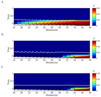
Figure 7.7 Velocity vectors distribution and salt concentration distribution at high tide for simulations: A) lowest dune height[HD1], B) the base case, and C) the largest dune height [HD5]. The aspect

ratio is 4 : 1. . . 78

Figure 7.8 Velocity vectors distribution andv velocity distribution at low tide for simulations: A) lowest dune height[HD1], B) the base case [Base], and C) the largest dune height [HD5]. The aspect

Figure 7.9 Velocity vectors distribution andv velocity distribution at high tide for simulations: A) lowest dune height[HD1], B) the base case [Base], and C) the largest dune height [HD5]. The aspect

ratio is 2 : 1. . . 80

Figure 7.10 Velocity vectors distribution and salt concentration distribution at low tide for simulations: A) lowest tidal amplitude [Ht1], B) the base case [Base], and C) the largest tidal amplitude [Ht4].

The aspect ratio is 4 : 1. . . 81

Figure 7.11 Velocity vectors distribution and salt concentration distribution at high tide for simulations: A) lowest tidal amplitude [Ht1], B) the base case [Base] case, and C) the largest tidal amplitude

[Ht4]. The aspect ratio is 4 : 1. . . 82

Figure 7.12 Velocity vectors distribution and v velocity distribution at low and high tide for simulations Ht4 with the largest tidal

ampli-tude. The aspect ratio is 2 : 1. . . 83

Figure 7.13 Average speed of the salt wedge in the dune field. . . 83

Figure 7.14 Effect of flow change, dune height change, and tidal amplitude change on the shear velocity over the dunes with the presence

of the salt wedge at high tide. . . 84

Figure 7.15 Effect of the river discharge change on the friction Richardson numberRit during low and high tide for simulations: A) lowest

discharge [Q1], B) the base case [Base] case, and C) the highest

flow [Q5]. . . 85

Figure 7.16 Effect of the dune height change on the friction Richardson numberRit during low and high tide for simulations: A)

small-est dune height [HD1], B) the base case [Base] case, and C) the

largest dune height [HD5]. . . 86

Figure 7.17 Effect of the tidal amplitude change on the friction Richard-son number,Rit, during low and high tide for simulations: A)

smallest tidal amplitude [Ht1], B) the base case [Base] case, and

C) the largest tidal amplitude [Ht5]. . . 87

Figure 7.18 Effect of the river discharge change on the internal Froude num-ber, F ri, during low and high tide for simulations: A) lowest

discharge [Q1], B) the base case [Base] case, and C) the highest

Figure 7.19 Effect of the river discharge change on the internal Froude num-ber,F ri, during low and high tide for simulations: A) smallest

dune height [HD1], B) the base case [Base] case, and C) the

largest dune height [HD5]. . . 89

Figure 7.20 Effect of the tidal amplitude change on the friction Richard-son number,Rit, during low and high tide for simulations: A)

smallest tidal amplitude [Ht1], B) the base case [Base] case, and

C) the largest tidal amplitude [Ht5]. . . 90

Figure 7.21 The variation of Froude number (F ri) vs. the dimensionless

height (H) under the effect of river discharge change. In this figure all the solid shapes represent for the values during high tide and the hollow shapes are for the low tide conditions. The boundaries separating the disturbances are based on experi-mental results compiled by Simpson (1999). The data points for Fraser River, and Seavalley are compiled by Kostaschuk et al. (2010) and Kostaschuk et al. (1992) respectively, and The

Orinoco point are based on the numbers in Ercilla et al. (2002). . 91

Figure 7.22 The variation of Froude number (F ri) vs. the dimensionless

height (H)under the effect of dune height change. In this figure all the solid shapes represent for the values during high tide and the hollow shapes are for the low tide conditions. The bound-aries separating the disturbances are based on experimental re-sults compiled by Simpson (1999). The data points for Fraser River, and Seavalley are compiled by Kostaschuk et al. (2010) and Kostaschuk et al. (1992) respectively, and The Orinoco

point are based on the numbers in Ercilla et al. (2002). . . 92

Figure 7.23 The variation of Froude number (F ri) vs. the dimensionless

height (H) under the effect of tidal amplitude change. In this figure all the solid shapes represent for the values during high tide and the hollow shapes are for the low tide conditions. The boundaries separating the disturbances are based on experi-mental results compiled by Simpson (1999). The data points for Fraser River, and Seavalley are compiled by Kostaschuk et al. (2010) and Kostaschuk et al. (1992) respectively, and The

Orinoco point are based on the numbers in Ercilla et al. (2002). . 93

Figure 8.1 Trapezoidal cross section in simulations Run1 and Run2. . . 102

Figure 8.3 Elevation contours for the three planforms tested with point

bar formation. . . 104

Figure 8.4 Schematic of the channel used in the current study. . . 105

Figure 8.5 Fine deposits distribution along the 30oangular amplitude chan-nel for A) trapezoidal cross section and Q=1.33 m3_{/s, and B)}

natural cross section and Q=1.33 m3_{/s. . . . 105}

Figure 8.6 Fine deposits distribution along the 90o_{angular amplitude}

chan-nel for A) trapezoidal cross section and Q=1.33 m3_{/s, and B)}

natural cross section and Q=1.33 m3_{/s. . . . 106}

Figure 8.7 Contour map for fine deposits thickness along the channel for 30o, 60o, and 90o angular amplitude. River flow is 1.33 m3_/s,

and the grain size used for suspended load is 30 µm. . . 107 Figure 8.8 Fine deposits distribution along the channel for A) angular

am-plitude = 45o_{, B) angular amplitude = 60}o_{, and C) angular}

amplitude = 75o_{. . . . 108}

Figure 8.9 Velocity magnitude distribution for the 30o_{, 60}o_{, and 90}o _{plan form. 109}

Figure 8.10 Velocity magnitude distribution and velocity vectors for 60o

planform cross section at A) the main channel apex, and B)

the center of the circulations down stream the main channel apex. 110

Figure 8.11 Effect of planform change on fine deposits partitioning over the

point bar. . . 111

Figure 8.12 Effect of planform change on the average deposition thickness

over the point bar. . . 112

Figure 8.13 Contour map for fine deposits thickness along the 30o _angular

amplitude channel for A)D=15 µm, B) D=30 µm C) D=50 µm. . 113 Figure 8.14 Contour map for fine deposits thickness along the 90o _angular

amplitude channel for A)D=15 µm, B) D=30 µm C) D=50 µm. . 114 Figure 8.15 Effect of suspended load grain size change on fine deposits

par-titioning over the point bar. . . 115

Figure 8.16 Effect of suspended load grain size change on the average

Figure 8.17 Contour map for fine deposits thickness along the 30o _angular

amplitude channel for A)Q=0.86 m3/s, B) Q=1.33 m3/s, and

C) Q=1.99 m3/s. . . 116

Figure 8.18 Contour map for velocity magnitude distribution at the first bend apex for A)Q=0.86 m3/s, B) Q=1.33 m3/s, and C) Q=1.99

m3/s. . . 117

Figure 8.19 Contour map for velocity magnitude distribution at the main bend apex for A)Q=0.86 m3/s, B) Q=1.33 m3/s, and C) Q=1.99

m3/s. . . 118

Figure 8.20 Contour map for velocity magnitude distribution at the center of the circulation in the main bend for A)Q=0.86 m3/s, B)

Q=1.33 m3/s, and C) Q=1.99 m3/s. . . 119

Figure 8.21 Effect of suspended load grain size change on fine deposits

par-titioning over the point bar. . . 120

Figure 8.22 Effect of suspended load grain size change on the average

de-position thickness over the point bar. . . 120

Figure 8.23 Contour map for fine deposits thickness along the 30o _angular

amplitude channel with Q=1.33 m3/s, D= 15µm and the slopes

used are A)0.22o _{and B) 0.022}o_{. . . . 121}

Figure 8.24 Contour map for fine deposits thickness along the 30o _angular

amplitude channel with Q=1.99 m3/s, D= 30µm and the slopes

used are A)1o _{and B) 0.1}o_{. . . . 121}

Figure 8.25 Effect of bed slope change on fine deposits partitioning over the

Chapter 1

Introduction

1.1 Free surface modeling

Numerical modeling of unsteady free surface flows has been a topic of academic and practical interest for many decades. In particular, dam-break flows have been studied extensively by solving the depth-averaged or Saint Venant equations using a variety of techniques such as method of characteristics, finite difference, finite element and finite volume (Katopodes and Strelkoff, 1978; Alam and Bhuiyan, 1995; Fraccarollo and Toro, 1995; Bradford and Sanders, 2002). The depth-averaged models elimi-nate the difficulty associated with modeling the free surface flow i.e. the interface between air and water and turbulence modeling in the vertical direction. These models are also computationally less expensive and are widely used in large scale applications such as storm surge modeling (Westerink et al., 1992; Blain et al., 1994). These advantages notwithstanding, depth-averaged models cannot be used for simu-lating stratified flow because of eliminating the vertical dimension by integrating the governing equations. These models also perform poorly in predicting supercritical flows with standing waves such as flow in open channel contractions (Rahman and Chaudhry, 1997; Jiménez and Chaudhry, 1988).

1.2 Open channel flow through transitions

transi-tions is an important design consideration. Separation is common in expansions due to a tendency for the flow to attach to one of the walls. Standing waves are common in supercritical flow passing through a contraction and pose the risk of flow overtop-ping. For obvious reasons, a depth-averaged model cannot reproduce flow separation which is a 3D flow phenomenon. A depth-averaged model can predict the occurrence of standing waves in open channel contractions but in previous works done by oth-ers (Jiménez and Chaudhry, 1988; Rahman and Chaudhry, 1997; Ladopoulos, 2010), shallow water models predicted water depths in channel contraction that differed considerably from measurements (Ippen and Dawson, 1951).

1.3 Mixing over bedform under low and high tide conditions

Estuaries are a dynamic environment experiencing continuous changes due to an interaction between the fresh water flow and salt wedge intruding from the ocean side. Tidal amplitude, the shape and properties of the bed forms, river flow variation due to the construction of hydraulic structures along the river or the seasonal changes in freshwater discharge, are factors controlling the mixing process, the water quality and morphodynamics in the estuarine environment (Farmer, 1951).

Estuaries can be classified on the basis of flow stratification or in other words water circulations in the estuaries. Majority of the estuaries have a brackish environment, with freshwater flow floating on top of the heavier saline water. Mixing between the freshwater discharge and saline water depends on several factors such as, the geometry of the estuary, tides, river discharge, and wind. Based on mixing the estuaries can be classified into four types: salt wedge, partially mixed, well mixed, and Fjord-type as shown in Figure 1.1 (Kennish, 1986).

bedforms affect the interfacial mixing between the fresh water and salt intrusions. Farmer (1951) illustrated the factors influencing mixing in estuaries: the river flow velocity, the mean total depth of water, the bed roughness, irregularities in the shape of the estuary, density difference between the fresh and salt water, and tidal currents.

1.4 Point bar Fine Deposits: Controls, Process and Pattern

Actively migrating sinuous or meandering rivers are common features of the fluvial landscape [Figure1.2]. Point bar deposits occur near the inner bank of a meandering channel bend due to helical flow which in turn results from an imbalance between centrifugal force and pressure gradient due to the superelevation of the free surface (Engelund, 1974; Kikkawa et al., 1976; Johannesson and Parker, 1989a,b; Kawai and Julien, 1996).

Point bars are sand rich objects which represent the reservoir for crude bitumen and oil reserves that exist in fluvial reservoirs. Accurate modeling for characterizing these fluvial reservoirs is challenging and complex due to the high level of hetero-geneity that exist within the fluvial deposits (Pranter et al., 2007; Jackson II, 1977; Labrecque et al., 2011). Discrete layers of mud and siltstone within the point bars act like baffles and therefore, humble the reservoir performance (Labrecque et al., 2011).

1.5 Motivations and objectives

surface flow is essential. Within point bar deposits, mud deposition as discrete layers has a significant effect on reservoir performance. Understanding the controls of mud layer deposition will help in producing more accurate models for oil reservoirs but the factors that affect the fine sediment partitioning in river systems are many and this makes the problem quite complex. The objectives of the proposed work are summarized below.

• Develop 3D and 2D models of unsteady free surface flows;

• Study 3D free surface flow in an open channel contraction by conducting

exper-iments and numerical model studies using both 3D and 2D models to resolve the mismatch between experimental data and numerical model results reported in the literature;

• Apply the numerical models to study interaction between an intruding salt

wedge and fixed bedforms under the influence of different tidal amplitude and freshwater discharge;

• Study the role of different controls on the fine deposit partitioning at in river

bends.

1.6 Organization of the Proposal

The remainder of this dissertation is organized as follows: In Chapter 2, the back-ground and a literature review of studies on open channel contraction, salt wedge intrusions and fine deposits on point bar is presented. In Chapter 3, the govern-ing equations and solution procedure for Reynolds-averaged Navier-Stokes equations (RANS) and a numerical method for tracking the free surface are presented.

In Chapter 5, the experimental set up and instrumentation for measuring water surface profiles in an open channel contraction are presented.

In Chapter 6, the flow field in an open channel contraction is studied using the depth-averaged and the 3D model. Results are compared with measurements done in the present study.

In Chapter 7, the effects of freshwater discharge, dune height and tidal amplitude on salt wedge migration and mixing between freshwater and the intruding salt wedge are investigated. The bottom boundary is considered to be fixed.

In Chapter 8, a study on the factors that control the fine deposits over river point bars is presented.

Chapter 2

Literature review

2.1 Open channel flow through transitions

Both expansion and contractions are used in hydraulic structures in order to facili-tate gradual transitions in channel cross sectional shapes and sizes. Both hydraulic jump and standing waves can occur in contractions and flow separation may occur in expansions.

Ippen and Dawson (1951) reported experimental measurements on supercritical flow through a contraction. Figure 2.1 shows a schematic of the experiment reported in Ippen and Dawson (1951) work, but the downstream straight part is longer.

the governing equations using the MacCormack second order accurate scheme, but the results did not improve (Figures 2.2, and 2.3).

Ladopoulos (2010) used the Singular Integral Operators Method (SIOM) to sim-ulate the free surface profile in open channel transitions by solving the Laplacean equation of potential flow. They compared their results with those from the works of Rahman and Chaudhry (1997), and Murty Bhallamudi and Chaudhry (1992), but did not present comparison with experimental measurements.

The fact that shallow water models of varied levels of accuracy failed to reproduce the experimental measurements of Ippen and Dawson (1951) leads to the following questions: i) are the data collected by Ippen and Dawson (1951) accurate or not? Measurement of free surface elevation of a supercritical flow with large Froude number by a point gauge may be prone to error; ii) are shallow water models based on finite differencing schemes inherently incapable of predicting free surface flows with standing waves? iii) are both of the above true? In this study, we address these questions by repeating the experiments of Ippen and Dawson (1951), solving the shallow water equations using a finite volume method with different flux limiters, and solving the 3D Reynolds-averaged Navier-Stokes equations for free surface flow.

2.2 Mixing over dune bed under tidal conditions

Mixing and sedimentation process in estuaries due to the interaction of salt wedge and tides have been studied through some field, experiential, numerical investigation. In the next section, a brief of these studies is provided.

Field studies

Fraser River Estuary, Canada, Kostaschuk et al. (2010) found that in an intruding salt wedge, mixing is restricted to the lower portion of the water column in the ab-sence of bedforms. This behavior changed dramatically once the salt wedge entered the dune field; mixing increased, the salt-wedge reached the water surface and large in-phase internal waves developed over the dunes. Figures 2.4, 2.5, and 2.6 show the measurement locations and shape of the salt wedge, over flat bed and over the dune field.

Sierra et al. (2004) studied the effect of discharge reduction in Ebro River due to flow diversion on the dynamics of the salt wedge and found that the salt wedge intru-sions will extend farther upstream in the river, and more problems with groundwater aquifers and crops can be expected.

Laboratory studies

Farmer (1951) conducted an experimental study to investigate the factors that affect the shape and length of the salt wedge over flat horizontal bed. Sargent and Jirka (1987) made detailed measurements of the vertical distribution of velocity and density for a steady saline wedge over a horizontal bed for different fresh water and saline flow discharges. Grigg (1995) studied the effect of spatial variation of the estuary cross section on the dynamics of the saline wedge by allowing a saline gravity current to propagate upstream against fresh flow from the upstream direction in a long, leveled flume containing contracting and expanding sections.

Numerical studies

models were used, for instance Fringer et al. (2006), Ralston et al. (2010), and Wang et al. (2011), solved Navier-Stokes equations with Boussinesq approximation.

Sylaios et al. (2006) developed a stratification-mixing model using water column potential energy (φ) based on the previous work of Simpson and Bowers (1981) and Nunes Vaz and Simpson (1994) to study the mechanisms controlling the vertical den-sity distribution at the mouth of a dam-controlled river. The model accounts for the influences of wind, solar heating, tidal circulation and river flow on the stratification. Liu et al. (2004) studied salt intrusions in an existing estuarine system. They inves-tigated the effect of the reduction in fresh water flow, and found that a significant increase in salinity has resulted from this change that may adversely affect the aquatic ecosystem in the lower reach of the estuary.

In some numerical studies the role of tidal cycle and topographic changes have been taken into consideration, but the main focus has been on the turbulent mixing in specific estuaries. Wang et al. (2011) modeled a field case, by considering the Sno-homish River, a microtidal salt wedge estuary, using the SUNTANS model. Ralston et al. (2010) found results similar to those by Wang et al. (2011), that the turbulent mixing of salt occurs generally during ebbs and is concentrated in the locations of the topographic transitions.

A systematic study to investigate the effects of river discharge, tidal amplitude, and dune height on mixing and the speed of salt wedge is needed to better understand the estuarine environment.

2.3 Point bar fine deposits: controls, process and pattern

Labrecque et al. (2011) studied a single channel and point bar deposits in the sub-surface of northeastern Alberta from Lower Cretaceous McMurray Formation which is one of the most important hydrocarbon accumulations in the world (Hubbard et al., 2011). The hydrocarbon reservoir quality in McMurray Formation is related to the overall thickness of the point bars and the vertical and spatial distribution of the siltstone beds. Also Labrecque et al. (2011) found that Siltstone bed thickness in the point bars increased downstream as the flow energy decreased and the suspended sediment in the flow deposited.

The fine deposits in the point bar can act like internal discontinuities for the reservoir body; an example can be found in a study of exposed point bar of the Williams Fork Formation in Coal Canyon, Piceance Basin, Colorado. (Pranter et al., 2007)

To the authors’ knowledge systematic studies for the factors controlling the fine deposits over point bars have not been done. Elucidating the underlying mechanisms of these discreet fine deposits layers will enhance the reservoir modeling accuracy and will improve the quality of the reservoir model. The problem with the existence of these layers is that many factors could be influencing their distribution and thickness. Kawai and Julien (1996) performed an experimental study for the point bar de-posits in narrow sharp bends. They showed that the configuration and size of the point bar depends on the sediment grain size. The point bar extended more in the down stream direction when fine sand was used. In another study Julien and Anthony (2002) found that the coarser sediments tend to go towards the channel thalweg and finer sediments move up the point bar, but Julien and Anthony (2002) did not ana-lyze the fine deposits distribution over the point bar and focused mainly on bed load transport.

upward and downstream fining sequences, and the nature of point bar, deposits is controlled by the seasonal flood deposition on bar surface and the pattern of channel migration.

River cross section in meandering channels changes from almost rectangular shape at inflection point along the river reach between two successive bends to an asym-metric shape. This asymmetry effect is quite important as it has a strong influence on the velocity pattern and ultimately the bed and planform morphology (Dietrich and Smith, 1983; Johannesson and Parker, 1989a).

During river bend migration the channel planform changes according to the migra-tion phase. The channel curvature is intricately related to bend migramigra-tion, strength of the helical flow, and point bar amplitude (Lagasse et al., 2004).

Factors affecting the fine sediment partitioning in river systems are many, for example bend radius of curvature, shape of the cross section, seasonal variation in river flow, grain size of the sediment, size of point bar, etc.

Figure 2.1: Plan view for the contraction experiment, all the dimensions are in meters

0 0.5 1 1.5 2 2.5 3 3.5

0 0.02 0.04 0.06 0.08 0.1 0.12

X(m)

H(m)

Ippen and Dawson, 1951 (Jiménez and Chaudhry, 1988 Rahman and Chaudhry, 1997

0 0.5 1 1.5 2 2.5 3 3.5 0 0.02 0.04 0.06 0.08 0.1 0.12 X(m) H(m)

Ippen and Dawson, 1951 (right wall) Ippen and Dawson, 1951 (left wall) (Jiménez and Chaudhry, 1988 Rahman and Chaudhry, 1997

Figure 2.3: Flow depth along the contraction wall.

INFLUENCE OF DUNES ON MIXING IN A MIGRATING SALT-WEDGE 461

freshet peak. Daily average discharge at Hope was 8440 m3 s−1 on 11 June and 7850 m3 _s−1 _{on 14 June, peaking at 11} 000 m3

s−1

on 23 June (Water Survey of Canada, 1999). The highest hourly tides at the Point Atkinson reference station were consistently around 4·5 m on 11–14 June, with the lowest tides decreasing from 0·9 m on 11 June to 0·16 m on 14 June (Canadian Hydrographic Service, 1999).

Measurements were collected from a launch travelling upstream along a navigation line in the center of the channel (Figure 1). Water depth and bedform geometry were measured with a 150 kHz Apelco® echo sounder and a SonTek® 1500 kHz, 3-beam acoustic Doppler profi ler (ADP) (Sontek/ YSI, San Diego) was used to measure the three-dimensional velocity at 5 s intervals. The ADP was tied to a Trimble® AgGPS Model 122 differential global positioning system (DGPS) (Trimble, Sunnyvale, CA). Szupiany et al. (2007) found that horizontal velocity measured with an aDcp should be averaged from at least fi ve transects, which was not possible in this study because of the rapid migration of the salt-wedge. Kostaschuk et al. (2004) conducted stationary tests with the system used here and found that velocity error was ±0·02 m s−1_, which suggests that the aDcp results are reasonable for the purposes of our investigation.

Results and Interpretation

The seaward (downstream) section of the study reach and survey line consists of a fl at bed with a gentle seaward slope (Figure 2), while the landward (upstream) section comprises a dune fi eld with an overall landward slope (Figure 3). A per-sistent bar develops in this reach of the channel (Villard and Church, 2003, 2005), with the fl at bed being located on the crest of the bar and the dune fi eld on the stoss (upstream-facing) side of the bar. An elevation difference of around 6 m exists between the crest and the deepest portion of the bar, which was ~1400 m in length at this time. The dunes have a longer landward-facing stoss side and a shorter, but steeper, seaward-facing lee side, refl ecting the dominance of down-stream sand transport at low tide (Kostaschuk and Villard, 1996). Dune size generally decreases upstream as water depth increases (Figure 3, Table 1) and dune heights, lengths and steepness are similar to those measured previously in the Main Channel (Kostaschuk and Villard, 1996; Villard and Church, 2003, 2005; Kostaschuk et al., 2004). Multitrack surveys con-ducted by Public Works Canada during high river fl ows (Villard and Church, 2003, 2005) reveal that the dunes are generally two-dimensional in planform but are more lunate in shape on the upper stoss side of the bar.

Figure 1. South Arm (Main Channel) of the Fraser River estuary, with

the survey transect shown as a dashed line. Sturgeon Bank and Roberts Bank are tidal fl ats.

Figure 2. Echosounding and ADP records along the survey line (see

Figure 1 for location). (a) 200 kHz echosounding trace; (b) horizontal velocity (u); (c) vertical velocity (v). X and Y labels on (a) refer to the plume at the head of the salt-wedge and interfacial waves respec-tively. Colour scale bars in (b) and (c) are in m s−1

. Distances are given from the Sand Heads Lighthouse (Figure 1). Positive and negative u indicate downstream (seaward) and upstream (landward) fl ow, respec-tively, while positive and negative v indicate vertical fl ow away from and towards the bed, respectively. This fi gure is available in colour online at www.interscience.wiley.com/journal/espl

Figure 3. Echosounding and ADP records along the survey line (see

Figure 1 for location). )a) 200 kHz echosounder trace; (b) horizontal velocity (u); (c) vertical velocity (v). X and Y labels on (a) refer to the plume at the head of the salt-wedge and interfacial waves over a dune respectively. Colour scale bars in (b) and (c) are in m s−1.Distances are given from the Sand Heads Lighthouse (Figure 1). Positive and negative u indicate downstream (seaward) and upstream (landward) fl ow, respectively, while positive and negative v indicate vertical fl ow away rom and towards the bed, respectively. This fi gure is available in colour online at www.interscience.wiley.com/journal/espl

Figure 2.4: Location of the field measurements by Kostaschuk et al. (2010) in Fraser River estuary.

INFLUENCE OF DUNES ON MIXING IN A MIGRATING SALT-WEDGE 461

freshet peak. Daily average discharge at Hope was 8440 m

_s

on 11 June and 7850 m

_s

_{on 14 June, peaking at 11}

000 m

_s

_{on 23 June (Water Survey of Canada, 1999). The}

highest hourly tides at the Point Atkinson reference station

were consistently around 4·5 m on 11–14 June, with the

lowest tides decreasing from 0·9 m on 11 June to 0·16 m on

14 June (Canadian Hydrographic Service, 1999).

Measurements were collected from a launch travelling

upstream along a navigation line in the center of the channel

(Figure 1). Water depth and bedform geometry were measured

with a 150 kHz Apelco® echo sounder and a SonTek®

1500 kHz, 3-beam acoustic Doppler profi ler (ADP) (Sontek/

YSI, San Diego) was used to measure the three-dimensional

velocity at 5 s intervals. The ADP was tied to a Trimble®

AgGPS Model 122 differential global positioning system

(DGPS) (Trimble, Sunnyvale, CA). Szupiany

et al.

(2007) found

that horizontal velocity measured with an aDcp should be

averaged from at least fi ve transects, which was not possible

in this study because of the rapid migration of the salt-wedge.

Kostaschuk

et al.

(2004) conducted stationary tests with the

system used here and found that velocity error was

±

0·02 m s

_,

which suggests that the aDcp results are reasonable for the

purposes of our investigation.

Results and Interpretation

The seaward (downstream) section of the study reach and

survey line consists of a fl at bed with a gentle seaward slope

(Figure 2), while the landward (upstream) section comprises a

dune fi eld with an overall landward slope (Figure 3). A

per-sistent bar develops in this reach of the channel (Villard and

Church, 2003, 2005), with the fl at bed being located on the

crest of the bar and the dune fi eld on the stoss

(upstream-facing) side of the bar. An elevation difference of around 6 m

exists between the crest and the deepest portion of the bar,

which was ~1400 m in length at this time. The dunes have a

longer landward-facing stoss side and a shorter, but steeper,

seaward-facing lee side, refl ecting the dominance of

down-stream sand transport at low tide (Kostaschuk and Villard,

1996). Dune size generally decreases upstream as water depth

increases (Figure 3, Table 1) and dune heights, lengths and

steepness are similar to those measured previously in the Main

Channel (Kostaschuk and Villard, 1996; Villard and Church,

2003, 2005; Kostaschuk

et al.

, 2004). Multitrack surveys

con-ducted by Public Works Canada during high river fl ows

(Villard and Church, 2003, 2005) reveal that the dunes are

generally two-dimensional in planform but are more lunate in

shape on the upper stoss side of the bar.

Figure 1. South Arm (Main Channel) of the Fraser River estuary, with

the survey transect shown as a dashed line. Sturgeon Bank and Roberts Bank are tidal fl ats.

Figure 2. Echosounding and ADP records along the survey line (see

Figure 1 for location). (a) 200 kHz echosounding trace; (b) horizontal

velocity (u); (c) vertical velocity (v). X and Y labels on (a) refer to the

plume at the head of the salt-wedge and interfacial waves

respec-tively. Colour scale bars in (b) and (c) are in m s−1_{. Distances are given}

from the Sand Heads Lighthouse (Figure 1). Positive and negative u

indicate downstream (seaward) and upstream (landward) fl ow,

respec-tively, while positive and negative v indicate vertical fl ow away from

and towards the bed, respectively. This fi gure is available in colour online at www.interscience.wiley.com/journal/espl

Figure 3. Echosounding and ADP records along the survey line (see

Figure 1 for location). )a) 200 kHz echosounder trace; (b) horizontal

velocity (u); (c) vertical velocity (v). X and Y labels on (a) refer to the

plume at the head of the salt-wedge and interfacial waves over a dune

respectively. Colour scale bars in (b) and (c) are in m s−1_.Distances

are given from the Sand Heads Lighthouse (Figure 1). Positive and

negative u indicate downstream (seaward) and upstream (landward)

fl ow, respectively, while positive and negative v indicate vertical fl ow

away rom and towards the bed, respectively. This fi gure is available in colour online at www.interscience.wiley.com/journal/espl

Figure 2.5: Field measurements by Kostaschuk et al. (2010) in Fraser River estuary; A) salt wedge propagation, B) u velocity, and c) v velocity over the flat part of the river bed.

INFLUENCE OF DUNES ON MIXING IN A MIGRATING SALT-WEDGE 461

Copyright © 2010 John Wiley & Sons, Ltd. Earth Surf. Process. Landforms, Vol. 35, 460–465 (2010)

freshet peak. Daily average discharge at Hope was 8440 m

_s

on 11 June and 7850 m

_s

_{on 14 June, peaking at 11}

000 m

_s

_{on 23 June (Water Survey of Canada, 1999). The}

highest hourly tides at the Point Atkinson reference station

were consistently around 4·5 m on 11–14 June, with the

lowest tides decreasing from 0·9 m on 11 June to 0·16 m on

14 June (Canadian Hydrographic Service, 1999).

Measurements were collected from a launch travelling

upstream along a navigation line in the center of the channel

(Figure 1). Water depth and bedform geometry were measured

with a 150 kHz Apelco® echo sounder and a SonTek®

1500 kHz, 3-beam acoustic Doppler profi ler (ADP) (Sontek/

YSI, San Diego) was used to measure the three-dimensional

velocity at 5 s intervals. The ADP was tied to a Trimble®

AgGPS Model 122 differential global positioning system

(DGPS) (Trimble, Sunnyvale, CA). Szupiany

et al.

(2007) found

that horizontal velocity measured with an aDcp should be

averaged from at least fi ve transects, which was not possible

in this study because of the rapid migration of the salt-wedge.

Kostaschuk

et al.

(2004) conducted stationary tests with the

system used here and found that velocity error was

±

0·02 m s

_,

which suggests that the aDcp results are reasonable for the

purposes of our investigation.

Results and Interpretation

The seaward (downstream) section of the study reach and

survey line consists of a fl at bed with a gentle seaward slope

(Figure 2), while the landward (upstream) section comprises a

dune fi eld with an overall landward slope (Figure 3). A

per-sistent bar develops in this reach of the channel (Villard and

Church, 2003, 2005), with the fl at bed being located on the

crest of the bar and the dune fi eld on the stoss

(upstream-facing) side of the bar. An elevation difference of around 6 m

exists between the crest and the deepest portion of the bar,

which was ~1400 m in length at this time. The dunes have a

longer landward-facing stoss side and a shorter, but steeper,

seaward-facing lee side, refl ecting the dominance of

down-stream sand transport at low tide (Kostaschuk and Villard,

1996). Dune size generally decreases upstream as water depth

increases (Figure 3, Table 1) and dune heights, lengths and

steepness are similar to those measured previously in the Main

Channel (Kostaschuk and Villard, 1996; Villard and Church,

2003, 2005; Kostaschuk

et al.

, 2004). Multitrack surveys

con-ducted by Public Works Canada during high river fl ows

(Villard and Church, 2003, 2005) reveal that the dunes are

generally two-dimensional in planform but are more lunate in

shape on the upper stoss side of the bar.

Figure 1. South Arm (Main Channel) of the Fraser River estuary, with

the survey transect shown as a dashed line. Sturgeon Bank and Roberts Bank are tidal fl ats.

Figure 2. Echosounding and ADP records along the survey line (see

Figure 1 for location). (a) 200 kHz echosounding trace; (b) horizontal

velocity (u); (c) vertical velocity (v). X and Y labels on (a) refer to the

plume at the head of the salt-wedge and interfacial waves

respec-tively. Colour scale bars in (b) and (c) are in m s−1_{. Distances are given}

from the Sand Heads Lighthouse (Figure 1). Positive and negative u

indicate downstream (seaward) and upstream (landward) fl ow,

respec-tively, while positive and negative v indicate vertical fl ow away from

and towards the bed, respectively. This fi gure is available in colour online at www.interscience.wiley.com/journal/espl

Figure 3. Echosounding and ADP records along the survey line (see

Figure 1 for location). )a) 200 kHz echosounder trace; (b) horizontal

velocity (u); (c) vertical velocity (v). X and Y labels on (a) refer to the

plume at the head of the salt-wedge and interfacial waves over a dune

respectively. Colour scale bars in (b) and (c) are in m s−1_.Distances

are given from the Sand Heads Lighthouse (Figure 1). Positive and

negative u indicate downstream (seaward) and upstream (landward)

fl ow, respectively, while positive and negative v indicate vertical fl ow

away rom and towards the bed, respectively. This fi gure is available in colour online at www.interscience.wiley.com/journal/espl

data are supplemented with high-quality 3-D seis-mic reflection data with a bandwidth of 8 to 220 Hz,

which cover the entire area of interest (Figure 2A).

The resolution of the seismic data set is considered to be <5 m (16.4 ft).

The McMurray Formation is characterized by a vertical stratigraphic succession shown to record an increasing marine influence upward (Mellon and Wall, 1956; Jeletzky, 1971). The stratigraphic architecture of sandstone bodies is variable, and

Figure 2.(A) Seismic time slice taken through the strata of interest, 8 ms (∼8 m [∼26 ft]) from a marine flooding surface present near the top of the McMurray Formation (indicated in Figure 1C). The white and yellow dots represent well locations, including those featured in this article (labeled). (B) Line-drawing trace of the main features in panel A. Some of the main depositional elements discussed are highlighted, including abandoned channel, point bar associated with lateral accretion (PBLA), point bar associated with downstream accretion (PBDA), counter point bar (CPB), and sandstone-filled channel. (C) Gamma-radiation map, constructed from values measured from wireline logs (wells used indicated with black dots) at the same stratigraphic interval of seismic time slice. The map provides a proxy for averaged lithology across the depositional elements observed in panels A and B. For example, the abandoned channels filled with siltstone stone are associated with the highest average gamma-radiation values observed.

1126 Seismic Geomorphology, Athabasca Oil Sands, Alberta by variations in seismic amplitude response that correspond to lithologic variability associated with ancient point-bar strata (Figure 2). These point-bar strata, or scrolls, are curved, and roughly parallel to the apex of the abandoned channel reaches in

which they are encapsulated (Figure 2). They are

oriented convex relative to the paleoflow direction. The main PBLA studied covers an area

approx-imately 4 × 3 km (2.3 × 1.9 mi;Figure 2B). The

stratigraphic succession represented by PBLA is up to 38 m (125 ft) thick, consisting of variable proportions of trough cross-bedded sandstone (Lf1) and interbedded sandstone and siltstone (Lf3) (Figure 5B, C). The Lf3 element is proportionally dominated by sandstone beds, which make up 65 to more than 95% of the depositional element (Figures 5B, C;6A). The coarsest part of the strati-graphic succession is located at the base, which is locally characterized by mudstone-clast

breccia-The PBLA is the most commonly interpreted depositional element in the McMurray Formation both in the subsurface and in outcrop and mining operations (e.g., Mossop and Flach, 1983; Strobl et al., 1997; Wightman and Pemberton, 1997; Hein et al., 2000). Interbedded siltstone and sandstone layers represent inclined heterolithic stratification (IHS) (cf. Thomas et al., 1987), which dip at 8 to 12° (cf. Muwais and Smith, 1990; Fustic, 2007). The IHS in the formation is widely considered to be tidally modified, formed in an estuarine setting (Smith, 1987, 1988, 1989). Marine influence on IHS deposits has also been supported through trace-fossil analysis in various McMurray Formation locations across northeastern Alberta (e.g., Pemberton et al., 1982; Ranger and Pemberton, 1988; Ranger and Gingras, 2003; Crerar and Arnott, 2007). The total thick-ness of PBLA packages is variable in the McMurray Formation, but based on the sharply defined bases

Figure 6.Stratigraphic cross sections through the channel and point-bar deposits using the marine flooding surface that overlies the channel package as a datum. Siltstone drapes locally extend through the entire point-bar package, partitioning the associated reservoir. See Figure 2Afor locations of cross section profiles.

Figure 2.7: Ancient point bar deposits of the McMurray Formation, Alberta, Canada (Hubbard et al., 2011).

Chapter 3

3D Numerical model

A 3D model with rigid lid boundary condition was developed at the University of South Carolina to study turbidity currents and the resulting morphological changes (Huang et al., 2005). The code is modified for free surface flows. The model solves the Reynolds-averaged Navier Stokes (RANS) equations and tracks and captures the free surface from the solution of the Volume of Fluids (VOF).

Reynolds-averaged conservation equations of fluid mass and momentum, conserva-tion of suspended sediment, transport equaconserva-tions of turbulent kinetic energy and its dissipation rate, boundary conditions and solution technique are presented. This is followed by a brief description of the interface capturing VOF equation and its solu-tion procedure, CICSAM (Ubbink and Issa, 1999). Finally, verificasolu-tion of the model is presented by simulating a case of 1D dam-break flow.

3.1 Governing equations

The Reynolds-averaged mass and momentum equations can be written as;

∂(ρuj)

∂xj

= 0 (3.1)

∂(ρuj)

∂t +

∂(ρuiuj)

∂xj

=− ∂p

∂xj

+ ∂

∂xj

µ∂uj ∂xj

−ρu0_iu0_j

!

+ρmgi (3.2)

whereui,uj = Reynolds-averaged velocities in the coordinate direction xi,xj

respec-tively; p= the Reynolds-average total pressure; ρm = the total density that includes

the fluid density and extra density due to the presence of salt or sediment,gi =

can as

−ρu0

iu0j =µt

∂ui

∂xj

+ ∂uj

∂xi

!

− 3

2ρkδij (3.3)

The eddy viscosity can be expressed as

µt=Cµρ

k2

ε (3.4)

whereCµ= constant of thek-εmodel;k= turbulent kinetic energy; andε= turbulent

dissipation rate. The two-equationk-εturbulence model modified for buoyancy effects (Rodi, 1984) used in the present study is expressed as

∂(ρk)

∂t +

∂(ρujk)

∂xj

= ∂

∂xj

"

µ+ µt

σk

_∂k

∂xj

#

−Gij −ρε+Gb (3.5)

∂(ρε)

∂t +

∂(ρujε)

∂xj

= ∂

∂xj

"

µ+ µt

σε

_∂ε

∂xj

#

+Cε1

ε

k(Gij+Gε3Gb)−Cε2ρ ε2

k (3.6)

where Gij is the generation term

Gij =−ρu0iu0j =ρνt

∂ui

∂xj

+ ∂uj

∂xi

!

∂ui

∂xj

(3.7)

Gb is the buoyancy term

Gb =−gi

ν σ

∂ρ ∂xi

(3.8)

The model coefficients are given as

Cµ = 0.09, Cε1 = 1.44, Cε2 = 1.92, σk = 1.0, σε= 1.3, σ= 0.85 (3.9)

The coefficient Cε3 is calculated according to Henkes et al. (1991):

Cε3 = tanh

u2 u1 (3.10)

whereu1,u2 is the local horizontal and vertical velocity component, respectively. The

mass conservation equation for solute or suspended sediment load can be expressed as

∂(ρc)

∂t +

∂(ρuj(uj−vsδj2)c)

∂xj

= ∂

∂xj

"

ρDm+

where c = Reynolds-average concentration; δj2 = Kronecker delta; with coordinate

j index 2 indicating the opposite direction of gravity; Dm = diffusion coefficient;

and Sct = turbulent Schmidt number. The shear velocity is computed based on the

following formula:

u∗ =C_µ1/4k1/2 (3.12) Bed level variation [∆ybed] can be estimated using the entrainment depositional rate

approach (Celik and Rodi, 1988; Imran et al., 1998)

∆ybed =

(D−E)dt

1−λ (3.13)

Where D is the sediment deposition rate and E is sediment entrainment rate. λis the porosity of bed sediment. D can be estimated using the following relation (Parker et al., 1986; Cesare et al., 2001)

D=cbvs (3.14)

Where cb and vs are the near bed concentration and the sediment fall velocity

respectively. E can be estimated by using Garcia and Parker (1993) relationship

E = AZ

5

1 +AZ5_/0.3vs (3.15)

A=1.3x10−7; Z= α1u∗Rpα2/vs; Rp =

q

RgDsgDsg/ν = particle Reynolds number;

Dsg= geometric mean size of sediment.

3.2 Boundary conditions

is applied for all the variables in the model except in the case of tidal boundary condition. At the top of the domain, a symmetry boundary condition is applied which means zero fluxes across the boundary, the domain is high enough that water does not reach to the top and the air velocity is small. At all the solid surfaces in the domain, wall boundary condition is used.

Concentration boundary condition is simple, as no solute is going to come out of the water so the concentration in the air region is set to zero, and flux of solute or sediment across the wall is also set as zero (Liu and García, 2008).

Tidal boundary condition is applied by defining the water depth at the outlet as a function of time. An increase in the water depth at the outlet will start to create a pressure difference between the downstream boundary and the the pressure inside the domain, and when there is enough pressure difference, water will start to get into the domain from the ocean side.

3.3 Solution procedure

The finite volume method for a nonorthogonal grid with collocated arrangement is used (Ferziger and Peric, 1999) to solve the governing equations. The current model uses the SIMPLEC algorithm (Van Doormaal and Raithby, 1984) to solve the conti-nuity and the momentum equations. More details of the algorithm can be found in Versteeg and Malalasekera (2007). The discretization for the unsteady term is done by using an implicit three time level scheme, which is a second order accuracte in time; a blended scheme is used for the dicretization of the convective fluxes through the cell faces.

at the faces, and other terms are determined to solve the continuity, momentum and then the turbulence model equations, and finally the mass conservation equations of solute and or suspended sediment are solved. After computing the new velocities, a check for the Courant number is done to adjust the time step if needed, then all of these steps are repeated until the end of the simulation. It is important to mention that the reason for using the Courant number condition is to keep the simulation stable as discussed in the following section.

3.4 Volume of fluid equation

The interface moves under the effect of the flow and in return affects the behavior of the flow. The difficulties in modeling the interfaces between two fluids lie in the need for a method that defines the interface position, the representation of the interface on a discrete grid, tracking of the spatial and temporal movement, the treatment of the partially filled cells, and coupling the interface conditions with the equations of motion (Ubbink, 1997).

Figure 3.1 illustrates the two categories of free surface modeling: surface methods or Lagrangian methods, and Volume method or Eulerian methods (Ferziger and Peric, 1999). The surface methods explicitly track the interface location throughout the simulation whereas the volume methods just mark the location of the fluids on either side of the free surface.

Many schemes have been developed for surface methods such as particles on in-terface (Daly, 1969), height functions (Nichols and Hirt, 1973), and level set method (Osher and Sethian, 1988; Sethian, 1999; Takizawa et al., 1992; Li and Zhan, 1993; Clarke and Issa, 1997).

fluid calculations (Daly, 1967), particle in cell (PIC) method (Harlow et al., 1976), and the grid-less method (Koshizuka, 1995). Although the particle in fluid can treat complex free surface shapes, this method requires significant amount of computer storage especially for three-dimensional simulations.

Schemes that use the volume of fraction concept depends on solving an equation for a scalar quantity that designates between the different fluids with a value that ranges between zero and one, where zero means that the cell is full of fluid number one, which is air in the present study, and one if the cell is full of fluid number two, which is water in the present study. Cells that have a value between zero and one are considered to be the surface cells (Ubbink, 1997).

Although the surface methods can track the exact location for the free surface, there is an important drawback of these methods that if the free surface starts to distort, the grid will need to be rearranged each time, which will require solution of another equation (Thompson et al., 1985), and the modified grid may be skewed and thus the simulation may diverge. In volume methods the computations are done on a fixed grid, so the skewness problem is not there, but the the free surface will be arbitrary shaped, and a finer grid is needed in the anticipated free surface region if a high resolution is required. Although the merges and fragmentation in the surface are taken care of, the surface shape might be smeared in a volume method (Shyy et al., 2007).

The volume fraction equation is expressed as

∂α ∂t +

∂(αuj)

∂xj

= 0 (3.16)

whereα is the fraction defined asα= the volume fluid 2 in the cell/the total volume of the cell. The fluid properties in the model i.e. local density and viscosity, are computed according to the following equations,

ρ=αρ1+ (1−α)ρ2 (3.17)

and

µ=αµ1 + (1−α)µ2 (3.18)

where 1 and 2 denote fluid one and fluid 2 which are water and air in the current study.

Equation 3.16, like other equations being integrated using finite volume method on an allocated grid, there is a need to interpolate the face values forαbased on the cell center values, but because of the special nature for the volume fractions equation as a step function, the chosen differencing scheme must preserve its discontinuous nature (Hirt and Nichols, 1981). The volume fraction face value, αf, can be interpolated

using the following equation

αf = (1−βf)αD +βfαA (3.19)

where αD is the volume fraction of the donor cell, αA is the volume fraction in the

acceptor cell, and βf is a weighting factor. Figure 3.2 represent a schematic for the

one-dimensional control volume and its neighbors. It is important to mention here that the order of the cells depends on the flow direction to determine which is the upwind cell (U), donor cell (D) , and the acceptor cell (A).

as line techniques (Noh and Woodward, 1976; Lötstedt, 1982; Youngs, 1982; Ashgriz and Poo, 1991), donor-acceptor formulation (Ramshaw and Trapp, 1976; Hirt and Nichols, 1981), and higher order differencing schemes (Ubbink and Issa, 1999).

Ubbink (1997) reported that the main limitation of the line techniques is that the reconstruction of the free surface on a rectangular grid is quite complex, while Ashgriz and Poo (1991) and Lafaurie et al. (1994) found that the donor acceptor formulation can deform and smear the shape of the free surface because it does not comply with local boundedness criteria as it does not take into account the upwind cell, and finally the higher order differencing schemes tried to overcome the problem of smearing the interface over several cells by minimizing the numerical diffusion produced by normal differencing. Ubbink (1997) developed a higher order compressive scheme which is widely used for modeling the interfaces. In the present work a high resolution method, compressive interface capturing scheme for arbitrary meshes (CICSAM) developed by Ubbink and Issa (1999) is used for capturing the free surface. The required steps to compute βf according to CICSAM is as follows

1. Compute the gradient (∇α)_D over the cell using Gauss’s theorem, (∇α)_D ≈ 1

VD n

X

f=1

Afαf (3.20)

where VD = the donor cell volume, Af = the face area vector, n = the total

number of cell faces.

2. Compute cD which is Courant number for all the cells,

cD = n

X

f=1

(

−Ffδt

VD

,0

)

(3.21)

where Ff = the volumetric flux at the cell face, and δt= the time step.

4. Predict ˜αD, the normalized variable for the donor cell,

˜

αD =

αD−αU

αA−αU

(3.22)

5. Estimate the normalized face value ˜αfCBC using the upper bound of the convec-tion boundedness criteria (CBC) (Gaskell and Lau, 1988; Leonard, 1991).

˜

αfCBC =

                       min       

1, α˜D cD       

when 0≤α˜D ≤1

˜

αD when α˜D <0,α˜D >0.

(3.23)

6. Estimate the normalized face value using the ULTIMATE-QUICKEST (UQ),

˜

αfU Q =

                       min        ˜

αfCBC,

8CDα˜D+ (1−CD)(6 ˜αD+ 3)

8       

when 0≤α˜D ≤1

˜

αD when α˜D <0,α˜D >0

(3.24) Ubbink (1997) introduced a weight factor,γf to take the free surface orientation

and the direction of the flow into account,

γf = min

       kγ

cos(θf) + 1

2 ,1        (3.25)

wherekγ is a coefficient that ranges between 0 to 1 andθf can be expressed as,

θf = arccos

(∇α)D ·df

|(∇α)D||df|

(3.26)

7. Calculate the normalized face value, ˜αf using the following equation,

˜

8. Compute βf the CICSAM weighting factor from the following equation,

βf =

˜

αf −α˜D

1−α˜D

(3.28)

9. After the weighting factor is obtained the only remaining step is to estimate the volume fraction face value using equation 3.19.

3.5 Model verification

Figure 3.1: Schematic of free surface computation methods; A) surface methods where the surface is tracked explicitly either by using marker points or by attaching the surface to the grid B) Volume methods where the fluid on either side of the surface are indicated by either massless particles or an indicator function Ubbink (1997)

.