University of South Carolina
Scholar Commons
Theses and Dissertations
2018
Environmental Impacts on Enterococcus in Shem
Creek, South Carolina, and Characterization of
Changing Land Use
Maria Elizabeth Zubizarreta University of South Carolina
Follow this and additional works at:https://scholarcommons.sc.edu/etd
Part of theEnvironmental Health Commons
This Open Access Dissertation is brought to you by Scholar Commons. It has been accepted for inclusion in Theses and Dissertations by an authorized
administrator of Scholar Commons. For more information, please [email protected].
Recommended Citation
E
NVIRONMENTALI
MPACTS ON ENTEROCOCCUS INS
HEMC
REEK,
S
OUTHC
AROLINA,
ANDC
HARACTERIZATION OFC
HANGINGL
ANDU
SESby
Maria Elizabeth Zubizarreta
Bachelor of Science College of Charleston, 2016
Submitted in Partial Fulfillment of the Requirements
For the Degree of Master of Science in
Environmental Health Sciences
The Norman J. Arnold School of Public Health
University of South Carolina
2018
Accepted by:
Geoffrey Scott, Director of Thesis
Dwayne Porter, Director of Thesis
Paul Pennington, Reader
Cheryl Carmack, Reader
Acknowledgements
I wish to acknowledge Geoff Scott, Dwayne Porter, Paul Pennington, and Cheryl
Carmack for their efforts in supporting and guiding me during this research project. I
would also like to thank Hilary Repick, from the Town of Mount Pleasant Public Service
Department’s Stormwater Division, for providing an accurate watershed outline for
Shem Creek and Lynn Shirley for his expertise working with Geographic Information
Abstract
Zoning and land-use practices have a direct influence on hydrologic systems and
can impact water resources. Linkages between change in land uses and degradation of
water quality in stream and watershed environments have been well established. Shem
Creek, located in Mount Pleasant, SC, has a history of fecal indicator bacteria levels that
exceed the Environmental Protection Agency’s recreational water quality standards. With
recent coastal population and development trends, proper management and the
sustainability of beach and estuary environments are a rising public health concern. The
objective of this study is to determine what climatic and water quality parameters are
associated with Enterococcus density levels and to characterize the changes in zoning
between 2010 and 2017 in the Shem Creek watershed. Public health implications of
development and impaired waters are also addressed. Geographic Information Systems
allowed for analysis of changes in zoning in the Shem Creek watershed between 2010
and 2017. Multivariate partial least squares regression was used to determine statistically
significant correlations between Enterococcus density levels and the following predictor
variables: water quality monitoring station location; month; water temperature, height,
and specific conductance; precipitation collected at two locations for 1, 2, and 3 days
leading up to Enterococcus sampling; and number of septic tanks located within a 0.5 and
1 mile radius of each water quality monitoring station. Because the amount of impervious
surface is directly related to water quality degradation, a change from zoning categories
surface was calculated. This equated to 3.2% of the total land area in the Shem Creek
watershed that changed from agricultural, recreational, vacant, or undevelopable to
commercial or residential. Results indicate that Enterococcus density levels have
increased over time and that precipitation and water height are positively correlated with
bacteria levels in Shem Creek. In addition, stations located further inland, where the
creek was surrounded by extensive marsh, had higher concentrations of Enterococcus
compared with stations located near the outflow of the creek into the harbor surrounded
by seawalls. Understanding what parameters are associated with increasing Enterococcus
density levels in Shem Creek will allow for future mitigation procedures to be
Table of Contents
Acknowledgements ... iii
Abstract ... iv
List of Tables ... vii
List of Figures ... ix
List of Abbreviations ... xi
Chapter 1: Introduction ...1
Chapter 2: Methods ...11
Chapter 3: Results ...20
Chapter 4: Discussion ...46
References ...55
Appendix A: Percent Variation Accounted for by Partial Least Squares Factors for All Models Leading Up to the Final Model Selected and Used for the Final Results ...61
List of Tables
Table 3.1 Percent Land Use by Zoning Category for the Shem Creek Watershed in 2010 and 2017 ...30
Table 3.2 Analysis of Variance for testing that the Rank Variables Reliably Predict the Transformed Enterococcus (ln(MPN)) Values in the Helsel’s Robust Method ...36
Table 3.3 Parameter Estimates for the Helsel’s Robust Method for Predicting Values of Enterococcus that Fell Below the Detection Limit (<10MPN/100ml) ...36
Table 3.4 All Variable Names Included in the Analysis and their Variable Description ..38
Table 3.5 Cross Validation for the Number of Extracted Factors ...38
Table 3.6 Descriptive Results of the Cross Validation for the Number of Extracted
Factors Process...39
Table 3.7 Percent Variation Accounted for by Partial Least Squares Factors ...39
Table 3.8 Parameter Estimates ...44
Table 3.9 Analysis of Variance for Testing that the Final Model Explains the Variance of the Response Variables ...45
Table A.1 Percent Variation Accounted for by the 2 Partial Least Squares Factors for Model 1 ...61
Table A.2 Percent Variation Accounted for by the 2 Partial Least Squares Factors for Model 2 ...62
Table A.3 Percent Variation Accounted for by the 2 Partial Least Squares Factors for Model 3 ...62
Table A.4 Percent Variation Accounted for by the 2 Partial Least Squares Factors for Model 4 ...63
List of Figures
Figure 2.1 Selected Shem Creek watershed ...17
Figure 2.2 Water quality monitoring station locations ...18
Figure 2.3 Septic tank locations ...19
Figure 3.1 Map of zoning categories in 2010 for the Shem Creek watershed ...29
Figure 3.2 Map of zoning categories in 2017 for the Shem Creek watershed ...30
Figure 3.3 Zoning categories that changed from agricultural, recreational, vacant, or undevelopable in 2010 to commercial or residential in 2017 in the Shem Creek watershed ...31
Figure 3.4 Natural log of Enterococcus density levels (ln(MPN)) included in the analysis graphed over time ...32
Figure 3.5 Number of septic tanks within a half-mile and a mile buffer or radius of each water quality monitoring station ...32
Figure 3.6 Number of Enterococcus density levels that exceeded the Class SB saltwater recreational limit for a single sample (501MPN/100ml) by year ...33
Figure 3.7 Number of Enterococcus density levels that exceed the Class SB recreational limit of 501MPN/100ml by month ...33
Figure 3.8 Distribution of the computed normal scores from the ranks for the transformed Enterococcus data ...34
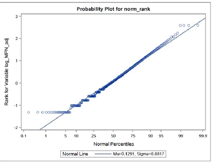
Figure 3.9 Probability plot for the computed normal scores from the ranks of the transformed Enterococcus data against normal percentile values ...35
Figure 3.10 Fit plot for the computed normal scores from the ranks and the transformed Enterococcus data ...36
Figure 3.11 Data points with uncensored (<10MPN/100ml) fitted values computed by Helsel’s Robust Method ...37
Figure 3.13 Correlation loading plot from Model 6, the final model, with lines drawn in for reading and analyzing the plot. ...41
Figure 3.14 Variable importance plot based on the Variance Importance for Projection (VIP) statistics of Wold for Model 6, the final model ...42
Figure 3.15 Regression coefficients profile of parameter estimates ...43
Figure 3.16 The distance to response and predictor models plot give the distance from each point to the PLS model with regard to the predictors first and then the responses ...44
Figure 4.1 Number of Enterococcus density levels that exceeded the Class SB saltwater recreational limit for a single sample (501MPN/100ml) by wet and dry climate ...53
List of Abbreviations
CV ...Coefficient of Variation (SAS code)
DEM ... Digital Elevation Model
EPA ... U.S. Environmental Protection Agency
GLM ... General Linear Model (SAS code)
LIDAR ... Light Detection and Ranging
MPN ... Most Probable Number
NOAA ... National Oceanic and Atmospheric Administration
PLS ... Partial Least Squares (SAS code)
PRESS ... Predicted Residual Error Sums of Squares
PROC ... Procedure (SAS code)
REG... Regression (SAS code)
SAS ... Statistical Analysis Software
SCDHEC ... South Carolina Department of Health and Environmental Control
SCDNR ... South Carolina Department of Natural Resources
Chapter 1
Introduction
Coastal shoreline counties in the United States (U.S.) account for 39% of the total
U.S. population and have grown steadily in recent decades (Crossett, Ache, Pacheco,
Haber, & National Oceanic and Atmospheric Administration, 2013). Population trends
indicate that there has been an increase of 40 million people living in coastline counties
in the U.S. between years 1960 and 2008 (Wilson, Fischetti, & U.S. Census Bureau,
2010). With population increases, development and urbanization of coastal areas will
play a fundamental role in the changes that occur within these coastal environments
(Brown, Johnson, Loveland, & Theobald, 2005). Anthropogenic changes to coastal
surroundings in the U.S. are increasing pollution, stimulating biological changes, and
compromising the sustainability and function of coastal ecosystems (Mallin, Williams,
Esham, & Lowe, 2000). The abundant supply of water in the form of streams, rivers,
wetlands, and lakes offers a rich source for outdoor recreational activities and has
significantly contributed to the development and growth of coastal state economies
(Haley, Parrish, Gaines, & South Carolina Department of Parks, Recreation, and
Tourism, 2014). In South Carolina (SC), beaches and coastal towns are the state’s
greatest attraction for the travel and tourism industry. However, the population in SC
coastal shoreline counties continues to increase (Wilson et al., 2010), and such growth
establishments, industrial sites, and transportation structures (Holland et al., 2004), which
can adversely affect the environmental quality of the state’s most precious resource.
Types of land uses and zoning have a direct influence on hydrologic systems and
can impact water resources (Lee, Hwang, Lee, Hwang, & Sung, 2009; Tong & Chen,
2002). Linkages between change in land uses and degradation of water quality in stream
and watershed environments have been established in many studies (DeFries &
Eshleman, 2004; DiDonato et al., 2009; Foley et al., 2005; Kelsey, Porter, Scott, Neet, &
White, 2004; Nelson, Scott, & Rust, 2005; Schoonover & Lockaby, 2006; Van Dolah et
al., 2008). Impervious surface cover (e.g., parking lots, roads, buildings) can cause
surface water to run directly into streams, rather than soaking into vegetation and soil
where it would undergo natural filtration (Holland et al., 2004). Urbanization presents a
unique threat to estuaries and coastal marshes that tend to be shallow where the rivers or
streams do not have adequate volumes of water to flush out pollutants (Vernberg, 1997).
Studies by Sanger, Holland, and Scott (1999b) indicate that when impervious cover
exceeds 10-20% of the inland region of the watershed near the headwaters, there are
changes in hydro-geography, salinity, sediment characteristics, and contaminant levels.
Van Dolah et al. (2007) documented that over 77% of the sites they sampled in SC
watersheds with >50% urban/suburban land cover had elevated sediment contaminant
concentrations; such results compared with only 27% of the sites they sampled with
≤30% urban/suburban land cover. Elevated levels of fecal coliform bacteria have also
been associated with urbanization and anthropogenic activity. Bacterial pollution
affecting estuaries, inlets, streams, and rivers is a rising environmental and public health
water temperatures. The elements that can contribute to bacterial growth and survival in
marine waters include salinity, temperature, predation, sunlight, toxic substances, and
nutrients. Estuaries offer ideal ranges for these factors and can additionally allow for
stresses in temperature or salinity, which might normally affect bacteria survival
negatively; however, such stresses are neutralized by the high nutrient content, enabling
persistent bacterial survival and growth (Apple, del Giorgi, & Kemp, 2006; Hendrickson,
Wong, Allen, Ford, & Epstein, 2001; Singleton, Attwell, Jangi, & Colwell, 1982).
Fecal bacteria including fecal coliform, Escherichia coli, and Enterococcus serve
as indicator species for health risk assessments and fecal bacteria pollution in water and
sediment bodies (Meays, Broersma, Nordin, & Mazumder, 2004). Fecal bacteria growth
is shown to increase in warmer temperatures making it a particular concern for the SC
coast where average water temperatures stay above 70°F for seven months and above
60°F for nine months out of the year (Howell, Coyne, & Cornelius, 1996; National
Oceanic and Atmospheric Administration, 2017). In 1976, the U.S. Public Health Service
and the U.S. Environmental Protection Agency (EPA) recommended fecal coliform
bacteria as an indicator for fecal bacterial contamination. The EPA later evaluated the use
of multiple organisms—including fecal coliform, E. coli, and Enterococcus—for fecal
indicator bacteria in epidemiological studies. These studies revealed that E. coli are good
predictors for gastrointestinal illness in freshwater and enterococci are good predictors in
marine and fresh recreational waters. The genus Enterococcus consists of gram-positive,
anaerobic organisms that are ovoid in shape and that are the current recommended fecal
indicator bacteria for marine and fresh recreational water standards published by the EPA
Leecaster, McGee, and Weisberg (2003) that tested three indicator species
(Enterococcus, total coliform, and fecal coliforms), Enterococcus was the indicator that
exceeded the recreational bacterial water quality standards the most.
Enterococci are part of the naturally occurring gastrointestinal flora that live in the
intestinal tracks of humans and wildlife. The public health concern occurs when these
bacteria contaminate recreational waters or waters where filter-feeding shellfish may be
harvested for human consumption. Swimmers are exposed to contaminants in water that
can easily enter the ears, eyes, nose, mouth, and other bodily openings as well as through
cuts or skin abrasions (Hendrickson et al., 2001). High fecal bacteria levels have also
been reported in the sand of wave-wash zones at public bathing beaches (Alm, Burke, &
Spain, 2003). Gastrointestinal illness and infections of the ear, eye, respiratory tract,
urinary tract, or skin among swimmers are directly associated with marine exposure and
marine bacterial counts (Balarajan, Raleigh, Yuen, & Machin, 1992; Prieto et al., 2001;
Pruss, 1998; Seyfried, Tobin, Brown, & Ness, 1985). Medical costs from these illnesses
due to marine exposures and the economic loss from beach closures and advisories
because of high bacteria levels in the water contribute substantially to public health
burdens in the United States (Given, Pendleton, & Boehm, 2006). Through gene transfer,
Enterococcus organisms have become inherently resistant to a number of antimicrobial
agents (Moellering, 1992). Exposure to antibiotics in the environment from agricultural
facilities and improper human disposal has generated the emergence of resistant
enterococci. Antibiotic resistant bacteria are of particular concern in hospital settings or
Bacterial contamination also poses a threat to marine organisms living in or
around coastal environments. Shallow tidal creeks and salt marshes act as nursery habitat
for fish and shellfish and provide feeding grounds for birds and predatory fish. Shellfish
such as oysters, clams, and mussels absorb nutrients by filtering water, thus absorbing
bacteria or other contaminants that may be in the water. These pollutants can become
concentrated in the shellfish, making them dangerous for raw human consumption
(Nelson et al., 2005). As a result, the South Carolina Department of Health and
Environmental Control (SCDHEC) has a shellfish harvesting monitoring program that
helps ensure the shellfish that are harvested meet the health and environmental quality
standards provided by federal recommendations and state guidelines (SC Department of
Health and Environmental Control, 2017d).
In addition to the shellfish monitoring program, SCDHEC has established the
ambient surface water quality monitoring program and the beach water quality
monitoring program. Each of these programs has its own standards and purpose but all
were created to meet the health and environmental quality standards provided by federal
guidelines and state regulations. SCDHEC’s standardized limit for enterococci in Class
SB tidal saltwater is 35 MPN (most probable number) per 100 ml (monthly average) and
501 MPN per 100 ml (daily maximum). In shellfish harvesting areas SCDHEC’s
standardized limit for fecal coliform is 14 MPN per 100 ml (monthly average) and 43
MPN per 100 ml (daily maximum). For enterococci in Class SA saltwater, the standard is
35 MPN per 100 ml (monthly average) and 104 MPN per 100 ml (daily maximum). Class
SA and SB tidal saltwater are suitable for primary and secondary contact recreation,
harvesting of clams, mussels, or oysters for market purposes or human consumption.
Class SA waters must maintain a higher dissolved oxygen level than Class B waters and
lower levels of single sample Enterococcus (SC Department of Health and
Environmental Control, 2014). The shellfish harvesting monitoring program provides a
database that is used to annually evaluate shellfish growing areas. This program includes
465 sample sites along the coast of South Carolina located in non-prohibited classified
shellfish areas (SC Department of Health and Environmental Control, 2017d). Shem
Creek is classified as a Class SB water body (SC Department of Health and
Environmental Control, 2017c). SCDHEC’s beach monitoring program consists of 123
beach-water monitoring stations that test for Enterococcus bacteria. The program began
monitoring state beaches routinely as a result of the federal Beaches Environmental
Assessment and Coastal Health Act of 2000. If high numbers of bacteria are found
(>501MPN), a swimming advisory for that portion of the beach is issued. If bacteria
levels are above 104 MPN but below 501 MPN, the sample will be re-tested. However,
advisories do not mean the beach is closed. Advisories are lifted when sample results fall
below 104 MPN per 100 ml. Samples are only taken during the swimming season (May 1
to October 1) (SC Department of Health and Environmental Control 2017a). SCDHEC’s
ambient surface water quality monitoring program takes a large variety of water quality
indicator measurements (including fecal indicator bacteria) and creates a database used to
understand the conditions of water bodies, how they can be improved, where closer
attention needs to be focused, and how permit limits for water discharge can be framed.
This program includes 145 permanent sites and additional sites chosen each year in both
2017b). Several ambient surface water quality monitoring sites are located in Shem Creek
and will be used in this study (SC Department of Health and Environmental Control,
2017c).
With recent coastal population and development trends, proper management and
the sustainability of beach and estuary environments must remain a priority. Public
policies for land use and water quality are progressively more interconnected (Abdalla,
2008). For example, wastewater treatment plants are required to meet technology-based
standards; farmers are encouraged to use best management practices that emphasize
fertilizer use and crop cover; and residential and commercial developers are encouraged
to control or manage stormwater runoff and prevent leaky septic systems. Zoning
categories—including commercial, industrial, residential, and agricultural sectors—often
incorporate policies limiting the number of buildings per acre and could be an approach
used for targeting land use in areas with compromised water quality. However, in some
areas concentrated development may actually have lower stormwater runoff compared
with large areas that are developed and more spread out; thus, policies that target
effective water quality improvement are not always clear (Walls & McConnell, 2004). In
addition, there are many different potential sources for bacterial contamination, both
point and non-point. Sources of human waste include improper disposal from waste water
treatment plants, poorly maintained septic systems, malfunctioning or failing sewer
infrastructure, and improper disposal of waste from marine boats (Scalf & Dunlap, 1997).
The South Carolina Department of Natural Resources implemented the Clean Vessel Act
Program in 1992, supporting a portion of the costs associated with the operation and
Natural Resources, 2016). Nevertheless, it is up to the boater to follow recommended
guidelines for waste disposal. Agricultural facilities can also be a source for bacterial
pollution in water due to storm water runoff. Wildlife and pet waste also contribute
substantially to bacterial contamination of waterways (Harwood, Whitlock, &
Withington, 2000). Despite the complexity of dealing with such multiple, varied sources
of contamination, there are several methods that can be used for microbial source
tracking to determine if the bacterial pollution is predominately anthropogenic or from
other animals (Scott, Rose, Jenkins, Farrah, & Lukasik, 2002).
Although many studies have looked at the relationship between change in land
uses and bacteria levels in marine waters, no studies have been published with a detailed
characterization of the bacterial levels and land uses surrounding Shem Creek. Shem
Creek, located in Mount Pleasant, SC, has had a history of fecal indicator bacteria levels
that exceed the EPA’s recreational water standards. Sanger, Holland, and Scott (1999b)
documented that in their study of 28 tidal creeks along the SC coast, Shem Creek had the
highest population density and largest percent of impervious surface.
1.1 Thesis Statement
The objective of this study is to investigate associations with higher Enterococcus
density levels in Shem Creek and to characterize the changes in zoning between 2010 and
2017 in the Shem Creek watershed. Public health implications of development and
impaired waters are also addressed. The null hypothesis is that there will be no
associations between Enterococcus density levels in Shem Creek and selected water
quality parameters, climatic occurrences, or other observations. A corollary of the null
the Shem Creek watershed. The alternative hypothesis is that there will be an association
between Enterococcus density levels in Shem Creek and selected water quality
parameters, climatic occurrences, or other observations. The alternative hypothesis also
has a corollary that zoning in the Shem Creek Watershed between 2010 and 2017
increased in developed impervious area and decreased in vacant or undeveloped
permeable area.
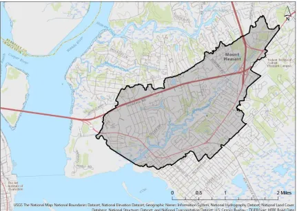
1.2 Study Area
Shem Creek is a tidal creek that empties into the Charleston Harbor on the coast
of South Carolina. It is known for its beautiful views, boardwalks, recreational use,
boating, and restaurants. Shem Creek runs though the town of Mt. Pleasant, which is
characterized by residential, commercial, agricultural, recreational, and other specialty
types of land use. The Shem Creek watershed is approximately 11.8 km2. Mt. Pleasant
had an estimated population of 82,215 in 2016, and population has been growing
exponentially since the 1960s. In the year 2016, 1,377 new dwellings were built and
1,622 were permitted (Town of Mount Pleasant Department of Planning and
Development, 2017).
Shem Creek was chosen as the study area because it has had persistently high
bacterial levels that surpass the recreational water quality standards. In 2016 SCDHEC’s
list of impaired waters listed Shem Creek with a priority 1 ranking for TMDL
development (SC Department of Health and Environmental Control, 2016). It is also a
popular destination for recreation and tourism. No direct sources have been established
for being the cause of bacterial contamination. There are no wastewater treatment facility
fisherman, and shrimp boats, so improper marine disposal of human waste and also leaky
septic tanks along the creek could be contributing factors towards the elevated fecal
bacteria levels. Pet and wildlife waste introduced via stormwater runoff is also a concern.
Shem Creek has been a site for shipbuilding, mill production, and factories,
providing varied economic support to the surrounding area throughout history (Moultrie
News, 2014). Shrimping became Shem Creek’s main industry in the 1930s when Captain
C. Magwood became the first fisherman to bring an ocean shrimp trawler into Mount
Pleasant. A bridge was built over Shem Creek and docks were constructed, allowing the
creek to develop into a major docking site for fisherman and shrimpers. Up to 70 shrimp
trawlers operated off these docks. Over time, this number has decreased significantly
because of increases in property tax and docking expenses. Today, Shem Creek is known
for its restaurants, bars, and recreation. Only ten fish and shrimp companies remain
actively working out of Shem Creek (Town of Mount Pleasant, n.d.).
This study first describes the methodology of determining a watershed for Shem
Creek and how geospatial zoning data were used to analyze changes in zoning over time.
Next, methodology of statistical analyses specifies positive and negative correlations
between water quality parameters; climatic factors, such as precipitation; location of
Enterococcus bacteria sampling; and Enterococcus density levels in Shem Creek. Finally,
results from statistical analyses performed are presented, concluding that Enterococcus
density levels in Shem Creek have increased over time. In addition, the research shows
that precipitation and water height are drivers for Enterococcus bacteria levels in Shem
Creek, with more concentrated bacterial pollution towards the headwaters as opposed to
Chapter 2
Methods
Methodology used for identifying an appropriate watershed for Shem Creek,
determining changes in zoning over time, and all statistical analyses performed in the
study are outlined in Chapter two.
2.1 Watershed Selection
There were three identified potential watersheds delineated for Shem Creek that
were taken into consideration before choosing the appropriate watershed for this study. A
watershed was delineated from a digital elevation model (DEM), using ArcGIS Pro’s
watershed tool. The Light Detection and Ranging (LIDAR) derived DEM was collected
from the National Oceanic and Atmospheric Administration’s (NOAA) Office for
Coastal Management and their Digital Coast Partnership Program. The outflow point
designated for the watershed was placed at the mouth of Shem Creek where it begins to
flow into the Charleston Harbor. In addition to the watershed delineated using ArcGIS
Pro’s watershed tool, there was a watershed boundary created by Charleston
Waterkeeper, using visual imagery. The selected watershed used for this study was
derived from the Town of Mount Pleasant Public Service Department’s Stormwater
Division (Figure 2.1). This watershed was created by on-the-ground mapping of the
hydrologic piping systems throughout the town. Because it takes into account the
man-made water pumping systems and water flow direction, this watershed was selected as the
2.2 Land Use and Zoning
Zoning data shapefiles for years 2010 and 2017 were acquired from Berkeley,
Charleston, and Dorchester Council of Government’s GIS office and clipped to the
boundaries of the Shem Creek watershed. Because the town of Mount Pleasant is highly
developed, detailed zoning data were used instead of generalized land cover maps. The
zoning shapefiles include description of each parcel for Charleston County. In the Shem
Creek watershed, 20 different property classifications were listed for year 2010, and 36
property classifications were listed for year 2017. Based on the details of the land use
files obtained, a new field or zoning classification system that made the 2010 and 2017
zoning files comparable was created using ArcGIS Pro. This field consisted of seven
categories: residential, commercial, recreational, agricultural, vacant, undevelopable, and
other (Appendix B). The summarize tool in ArcGIS Pro was used to sum the square area
of land in each category. The percent of each category within the Shem Creek watershed
was derived by dividing the land area of each category into the total land area of the
watershed. In addition, a spatial join between the 2010 and 2017 zoning files was created.
Using the summarize tool, the sum of land area within the new land use field
classifications that changed from 2010 to 2017 was calculated. This allowed for
determination of how much land changed from one category (e.g., vacant) to another
(e.g., residential). Final production of color-coded maps to create visual representation of
this change was created and exported from ArcGIS Pro.
2.3 Variable Selection
Values for Enterococcus density were obtained from four water quality
Enterococcus density levels in recreational swimming areas around Charleston on a
weekly basis during the months of May through October since in 2013. Charleston
Waterkeeper has three water quality monitoring stations located in Shem Creek (Shem
Creek station 1, 2, and 3). SCDHEC previously measured Enterococcus as part of routine
surveys for its ambient water quality monitoring program in one location within Shem
Creek (RT-10116 station). In 2010, Enterococcus density levels were collected monthly
from SCDHEC’s water quality monitoring station. Enterococcus data was not collected
for years 2011 and 2012. Observed Enterococcus densities were calculated using
standardized methods. A total of 372 water sample results were included in the analysis:
13 readings from site RT-10116; 120 readings from Shem Creek 1; 119 readings from
Shem Creek 2; and 120 from Shem Creek 3. The station, date, and time were recorded for
each sample. SCDHEC’s standardized limit for enterococci in Class SB tidal saltwater,
which is a monthly average of 35 MPN per 100 ml and a daily maximum of 501 MPN
per 100 ml, was used to complete analyses in this study (SC Department of Health and
Environmental Control, 2014).
Water temperature (°C) and specific conductance (μS/cm) were collected from a
U.S. Geological Survey’s water quality monitoring station located in the Cooper River
near the U.S. Customs House in downtown Charleston. Values were collected every 15
minutes. The nearest value to the time of Enterococcus sample collection was used.
Verified water height (ft) was collected by a NOAA water quality monitoring station,
also located in the Cooper River near the U.S. Customs House in downtown Charleston.
Values were recorded every six minutes. The closest value to the time of each
two NOAA site locations: one in downtown Charleston at the U.S. Customs House and
the other at the Charleston International Airport located in North Charleston. Because
most Enterococcus density samples were collected in the mornings, rainfall data were
summed by the total number of inches of rain during the previous day, two days, or three
days leading up to Enterococcus sample collection. The number of septic tanks was
approximated by those businesses or homes that were not connected to the municipal
sewage system but that had running water (Figure 2.3). The number of septic tanks
located within a half mile and a mile radius of each Enterococcus water quality sampling
station was calculated.
2.4 Statistical Analysis
Analyses were performed using SAS 9.4 (SAS Institute Inc., Cary, NC).
Enterococcus data were ln(x) transformed prior to analysis to obtain normality and
homoscedasticity. The natural log was chosen because it best represents the way that
bacteria multiply in the water. Helsel’s Robust Method was used to assign a value to any
Enterococcus density measurements that were below the limit of detection
(<10MPN/100ml). This method has been frequently used and is well established for
dealing with non-detection values in water quality samples (Helsel & Cohn, 1988;
Newman, 1995). The methods consisted of a series of steps in order to assign a value
based on a normal distribution curve for those values under the limit of detection. First,
the data were ranked and transformed to compute normal scores from the ranks. The
resulting ranks appear normally distributed (SAS Institute Inc., 2009a). All ties in
Enterococcus observations were assigned a mean averaged rank score. The PROC
fit a normal curve. PROC REG was used to generate a prediction equation, which could
then be used to predict the values below the detection limit (<10MPN/100ml). Results
from this method were verified using UnCensor v4.0 (Newman & Dixon, 1990), a
program designed specifically for this type of environmental analysis (Newman, 1995).
Multivariate partial least squares (PLS) regression was used to determine
statistically significant associations between Enterococcus density level and the
following input variables: sampling station; month; water temperature; water height;
specific conductance; rainfall for 1, 2, and 3 days leading up to sampling at two locations
(U.S. Customs House and Charleston International Airport); and number of septic tanks
located within a 0.5 and 1 mile buffer of each sampling station. The PLS procedure was
used to carry out this analysis. All of the methods executed in PROC PLS work by
obtaining consecutive linear combinations of the predictors. These are called factors,
which explain the variation in both the response and predictor variables. Factors are
extracted from a matrix, which includes both the predictor and response variables. A
one-at-a-time cross validation method was used to choose the number of extracted factors to
fit the model specified by the CV=ONE option. This option requires a re-calculation of
the PLS model for every entered observation. The absolute minimum PRESS (predicted
residual error sums of squares) is achieved with the number of extracted factors that have
a statistically significant p-value less than 0.05. The PRESS statistic is a form of
cross-validation used in regression analysis as a measure of the fit of a model and is based on
the residuals generated from calculating the sums of squares of the prediction residuals
for each observation in the model (SAS Institute Inc., 2013). The CVTEST option was
residuals from different models are significant. This methodology, proposed by Van der
Voet (1994), extracts the smallest number of factors that have residuals insignificantly
larger (p >.1) than the residuals of the model with minimum PRESS.
The PLS procedure outputs a variable importance plot, which based on
the Variable Importance for Projection (VIP) statistic of Wold (Wold, 1995), displays the
influence of each predictor variable in fitting the PLS model for the predictors and
response variables. According to Wold, when a predictor variable has a small coefficient
(in absolute value) and a small VIP (less than 0.8) value, it is a suitable candidate for
deletion (SAS Institute Inc., 2009b). Predictor variables that fell below 0.8 on the
variable importance plot were dropped from the model and the PLS procedure was
re-run. This process was repeated until the best model explaining the variance in the
predictor and response variables was found. The results from the PLS procedure were
Chapter 3
Results
Chapter three describes results for changes in zoning in the Shem Creek
watershed between 2010 and 2017, multiple trends associated with Enterococcus density
levels in Shem Creek, and positive or negative correlations between water quality
variables and Enterococcus.
3.1 Land Use and Zoning
Shem Creek was categorized by seven zoning descriptions. Figures 3.1 and 3.2
show the zoning categories for 2010 and for 2017. The zoning categories that would
likely contain the highest amount of impervious surface on the lot would be commercial
and residential. In contrast, the zoning categories that would contain the least amount of
impervious surface would be agricultural, vacant, recreational, and undevelopable
(Arnold & Gibbons, 1996). Table 3.1 represents the percent of land area described by
zoning in the Shem Creek watershed in 2010 and 2017. In the Shem Creek watershed, the
largest percent of land area consisted of residential zoning areas: 82.2% (2010) and
83.9% (2017). The percent of land area that was zoned as vacant in 2010 equated to
10.3%, which decreased to 8% in 2017. When comparing 2010 to 2017, 69.3% of the
land area in the Shem Creek watershed stayed as the same zoning classification. Because
the amount of impervious surface is directly related to water quality degradation (Foley et
to 3.2% of the total land area in the watershed that changed from agricultural,
recreational, vacant, or undevelopable in 2010 to commercial or residential in 2017
(Figure 3.3).
For each zoning category, the largest change in square area was calculated as follows:
• 2.36km2 of land that was categorized as commercial in 2010 changed to
residential zoning in 2017
• 39.48km2 of land that was categorized as residential in 2010 stayed as residential
zoning areas in 2017
• 5.17km2 of land that was categorized as other in 2010 changed to residential
zoning areas in 2017
• 0.91km2 of land that was categorized as undevelopable in 2010 changed to
residential zoning areas in 2017
• 0.51km2 of land that was categorized as vacant in 2010 changed to residential
zoning areas in 2017
• 0.02km2 of land that was categorized as recreational in 2010 stayed as
recreational zoning areas in 2017
• 0.05km2 of land that was categorized as agricultural in 2010 changed to vacant in
2017
3.2 Descriptive Results for Water Quality Analysis
Figure 3.4 displays a plot of the natural log transformed Enterococcus density
levels (MPN), excluding those that fell below the detection limit, which are later
accounted for and included in this study. The highest values of Enterococcus density
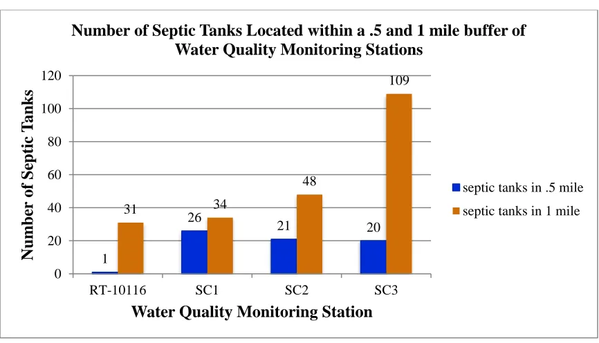
samples taken over time. Shem Creek station 3 (SC3) had the highest amount of septic
tanks located within one mile (n=109), but Shem Creek station 1 (SC1) had the highest
amount of septic tanks located within a half-mile radius (n=26). All septic tanks located
within a one or half-mile buffer of each station can be seen in Figure 3.5. The number of
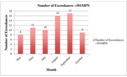
Enterococcus density levels that exceeded the state daily maximum for recreationally
used Class SB tidal saltwater (<501MPN/100ml) has increased over time with most of
these exceedances occurring in September, followed closely by August (Figures 3.6 and
3.7).
3.3. Helsel’s Robust Method Statistical Results
Of the total of 372 samples of Enterococcus analyzed in this study, 23 were below
the detection limit (<10MPN/100ml) equating to 6.18% of the total sample size. In the
tests for normality of the ranked transformed Enterococcus (ln(MPN)) values, the
Shapiro-Wilk test statistic had an associated p-value of <0.0001. Statistically significant
p-values are defined as those less than α=0.05. Because the p-value was statistically
significant, the null hypothesis that there was no significant departure from normality was
rejected, concluding that the ranks assigned to the transformed Enterococcus (ln(MPN))
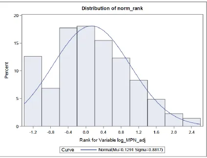
values fit a normal distribution. The distribution of the ranks was slightly positively
skewed because of the number of ties in the data set (Figure 3.8). Figure 3.9 displays
where the ties occurred on the normal distribution curve. The F-value in the analysis of
variance (Table 3.2) was statistically significant (p-value <0.0001), indicating that the
rank variables reliably predict the transformed Enterococcus (ln(MPN)) values. The
R-Square value, which indicates the proportion of variance in the dependent variable
was 0.9791. Figure 3.10 displays how closely the data for transformed Enterococcus
(ln(MPN)) and the computed ranked scores fit together. Based on the parameter estimates
(Table 3.3), a prediction equation was computed to assign values for those Enterococcus
data points that were under the detection limit (<10MPN/100ml). These assigned values
are displayed in Figure 3.11.
3.4 Multivariate Partial Least Squares Regression Results
Multivariate partial least squares (PLS) regression was used to determine
statistically significant associations between Enterococcus density levels and the
variables listed in Table 3.4. A total of six different models were run in order to
determine the best-fit model. The following paragraphs walk through the model selection
process and results of the PLS procedures.
The variable “month” was taken out of the model because there were months in
year 2010 that did not have observations for any of the other years. When the PLS
procedure was run with “month” in it, there were no significant factors extracted, which
prevented the analysis from working appropriately or presenting any results. The PLS
procedure was re-run, excluding “month” from the model. In this model (Model 1), there
were two statistically significant factors extracted (factor 1: value <0.0001, factor 2:
p-value 0.008). Appendix A displays the percent variation accounted for by the partial least
squares factors for each variable in all the models tested leading up to the final selected
model. The following six variables in Model 1 fell below Wold’s criteria of 0.8 in the
variable importance plot: station SC2, precipitation values from the Charleston
International Airport, water temperature, and number of septic tanks located within a half
The PLS procedure was re-run, excluding all precipitation values from the
Charleston International Airport, water temperature, and number of septic tanks located
within a half mile of each station (Model 2). Station SC2 was not excluded from the
model even though it fell below Wold’s criteria because this was a categorical variable.
Taking out SC2 would exclude 119 observations, equating to almost a third of the total
data set used in this study. In Model 2—which included all stations, all precipitation data
for the downtown U.S. Charleston Customs House, conductivity, water height, and septic
tanks located in a one-mile buffer of each station—there were two statistically significant
factors extracted (factor 1: p-value <0.0001, factor 2: p-value 0.014). Station SC2 still fell
below Wold’s criteria of .8 on the variable importance plot.
Because station RT-10116 contained observations from only the year 2010 and
none of the other years, it was taken out of the model to make sure this station was not
skewing the results. The PLS procedure was re-run excluding station RT-10116 (Model
3). Model 3 included stations SC1, SC2, and SC3; all precipitation data from the
downtown Charleston U.S. Customs House; conductivity; water height; and septic tanks
located within a one-mile buffer of each station. Model 3 extracted two statistically
significant factors (factor 1: p-value <0.0001, factor 2: p-value 0.044). Because the
percent variation accounted for by the partial least squares factors did not change
substantially for the predictor values (totals: 36.93 for Model 2 and 41.38 for Model 3),
keeping station RT-10116 in the model remains appropriate in order to keep observations
from year 2010.
Before adding station RT-10116 back into the model, station SC2 was also
results. This was done because station SC2 fell below Wold’s criteria of 0.8 in the
variable importance plot for all the previous models. In this effort to analyze what results
would be produced by excluding these observations, the PLS procedure was re-run
excluding both station SC2 and station RT-10116 (Model 4). Model 4 extracted two
statistically significant factors (factor 1: p-value <0.0001, factor 2: p-value 0.064). Model
4 included station SC1 and SC2, all precipitation data from the downtown Charleston
U.S. Customs House, conductivity, water height, and septic tanks located within a
one-mile buffer of each station. Precipitation values two and three days before sample
collection and conductivity fell below Wold’s criteria of 0.8 but only by about a tenth of
a decimal. Because taking out station SC2 excluded so many observations in the data set,
both station SC2 and station RT-10116 should be added back into the model.
After considering the data further, it was realized that because the number of
septic tanks located in a 1-mile buffer around each station was a constant value for each
station, this was essentially a weighted numerical value assigned for the variable
“station.” Therefore, the number of septic tanks was taken out of the model completely.
The PLS procedure was re-run (Model 5) and extracted two statistically significant
factors (factor 1: p-value <0.0001, factor 2: p-value 0.001). Model 5 included stations
RT-10116, SC1 and SC2; all precipitation data from the downtown Charleston U.S.
Customs House; conductivity; and water height. All variables except for station SC2
remained above Wold’s criteria of 0.8 on the variable importance plot. In Model 5,
conductivity was just slightly above Wold’s criteria of 0.8 on the variable importance
plot. In addition, only 15.48% of the variation accounted for by the partial least squares
In an effort to obtain a model in which the predictor variables in the model
explain the highest percent of variation, conductivity was excluded from the model and
the PLS procedure was re-run (Model 6). In Model 6, the variation summary shows that
the two factors in the model explain 46.71% of the total predictor variation and 43.16%
of the response variation. The percent variation accounted for by the predictor variables
increased with Model 6, compared to Model 5, which was 42.44%. Therefore, Model 6
appeared to be the best-fit model. Because there were several missing observations in the
precipitation data set, PROC PLS excluded these from the analysis, and no predictions
were computed for those missing observations. The final model contained 367 records of
observations used in the final analysis. In Model 6, the absolute minimum PRESS was
achieved with two extracted factors that have a statistically significant p-value less than
0.05 (factor 1: p-value <0.0001, factor 2: p-value 0.002). The complete factor selection
process is shown in Tables 3.5 and 3.6. The percent variation accounted for by the partial
least squares factors in the final model is shown in Table 3.7.
The correlation loading plot summarizes the two factors and the features in the
PLS model, displaying the primary results (Figure 3.12). This plot is composed of
blanketed scatter plots, which include the variation explained by both factors for each
variable and the weighted effects of the model (SAS Institute Inc., 2009b). The amount of
variation explained by the model for each of the variables is comparable to the distance
from the origin of the plot. The transformed Enterococcus levels, represented by their
observation number in the data set on this plot, are randomly clustered towards the origin,
indicating that the data contribute appropriate information about the two factors. Drawing
origin and the response variable produces relative positive and negative correlations
between the predictor and response variables. Figure 3.13 displays the drawn lines that
were used to interpret the plot. The correlation loading plot indicates that station SC3 is
highly positively correlated with the transformed Enterococcus density levels (labeled
“log_MPN_adj” on the plot). Station SC3 was the most correlated with the transformed
Enterococcus density levels compared to all other predictor variables in the model. Water
height values followed closely by precipitation are also positively correlated with the
transformed Enterococcus density levels. Station SC2, which is located towards the
origin of the plot, has no correlation with the transformed Enterococcus density levels.
Station RT-10116 is slightly negatively correlated with the transformed Enterococcus
density levels. Station SC1 is also negatively correlated with the transformed
Enterococcus density levels.
All variables in the final model, except for station SC2, remained above Wold’s
criteria of 0.8 on the variable importance plot (Figure 3.14). As stated previously, station
SC2 was kept in the model to avoid eliminating almost a third of the data set. The
regression coefficients profile in Figure 3.15 signifies the importance each predictor
variable has in the prediction of only the response variable. In the regression coefficients
profile plot, station RT-10116 and SC1 have negative coefficients. Looking back at the
correlations loadings plot, these are the variables that tend to be negatively correlated
with the dependent variable. The plot shown in Figure 3.16 gives the distance from each
point to the PLS model with regard to the predictors first and then the responses. This
allows for identification of potential outliers. Points that are dramatically farther from the
to the right on the X-axis of this plot are potential outliers. However, because of the
reliable methods for reading Enterococcus density levels and because of the many factors
that can drastically impact Enterococcus density levels in water, these were not excluded
from the analysis. The parameter estimates that are used to create the prediction equation
are displayed in Table 3.8.
In order to confirm that the PLS procedure analysis results were accurate, the
GLM procedure was run, using the same data from the final model. The F-value in the
analysis of variance (Table 3.9) was statistically significant (p-value <0.0001), indicating
that the model does explain the variance of the response variables. The R2, which is the
total variance explained by the model was 0.462199 (46.22%). This remains very close to
the variation summary from the PLS procedure in Model 6 that concluded 46.71% of the
Figure 3.2: Map of zoning categories in 2017 for the Shem Creek watershed
Table 3.1: Percent land use by zoning category for the Shem Creek watershed in 2010 and 2017
Zoning Category 2010 (% cover) 2017 (% cover)
Commercial 3.5 2.3
Residential 82.2 83.9
Vacant 10.3 8.0
Recreational 1.5 1.6
Agricultural 0.0 0.0
Undevelopable 0.9 1.3
Figure 3.4: Natural log of Enterococcus density levels (ln(MPN)) included in the analysis graphed over time. This figure excludes Enterococcus density levels that fell below the detection limit (<10MPN/100ml).
Figure 3.5: Number of septic tanks within a half-mile and a mile buffer or radius of each 0 2 4 6 8 10 12 ln (M P N) Date Enterococcus (MPN) 1 26 21 20 31 34 48 109 0 20 40 60 80 100 120
RT-10116 SC1 SC2 SC3
Num b er of S ep tic T an k s
Water Quality Monitoring Station
Number of Septic Tanks Located within a .5 and 1 mile buffer of Water Quality Monitoring Stations
septic tanks in .5 mile
Figure 3.6: Number of Enterococcus density levels that exceeded the Class SB saltwater recreational limit for a single sample (501MPN/100ml) by year
Figure 3.7: Number of Enterococcus density levels that exceed the Class SB saltwater recreational limit of 501MPN/100ml by month
1 6 14 14 16 22 0 5 10 15 20 25
2010 2013 2014 2015 2016 2017
Num b er of E xc ee d an ce s Year
Number of Exceedances >501MPN
Number of Exceedances >501MPN 8 11 10 16 17 9 0 2 4 6 8 10 12 14 16 18 Num b er of E xc ee d an ce s Month
Number of Exceedances >501MPN
Figure 3.9: Probability plot for the computed normal scores from the ranks (norm_rank) of the natural log transformed Enterococcus data (log_MPN_adj) against normal
Figure 3.10: Fit plot for the computed normal scores from the ranks (Rank for Variable log_MPN_adj) and the natural log transformed Enterococcus data (log_MPN_adj)
Table 3.2: Analysis of Variance for testing that the Rank Variables Reliably Predict the Transformed Enterococcus (ln(MPN)) Values in the Helsel’s Robust Method
Source DF Sum of Squares Mean Square F Value Pr > F
Model 1 996.07825 996.07825 16231.2 <0.0001
Error 347 21.29479 0.06137
Corrected Total 348 1017.37304
Table 3.3: Parameter Estimates for the Helsel’s Robust Method for Predicting Values of Enterococcus that Fell Below the Detection Limit (<10MPN/100ml)
Variable Label DF Parameter
Estimates
Standard Error
t value Pr > |t|
Intercept Intercept 1 4.72752 0.01340 352.74 <0.0001 norm_rank Rank for Variable
log_MPN_adj
Figure 3.11: Data points with uncensored (<10MPN/100ml) fitted values computed by Helsel’s Robust Method
6.18%
Table 3.4: All Variable Names Included in the Analysis and Their Variable Description
Variable Name Variable Description
RT-10116 Water quality monitoring station SC1 Water quality monitoring station SC2 Water quality monitoring station SC3 Water quality monitoring station
Month Month
Rain_1d_airport Total precipitation on the day prior to water sample collection at the Charleston International Airport
Rain_2d_airport Total sum of precipitation on the 2 days prior to water sample collection at the Charleston International Airport
Rain_3d_airport Total sum of precipitation on the 3 days prior to water sample collection at the Charleston International Airport
Rain_1d_dt Total precipitation on the day prior to water sample collection at the Charleston Clearing House, located Downtown
Rain_2d_dt Total sum of precipitation on the 2 days prior to water sample collection at the Charleston Clearing House, located Downtown Rain_3d_dt Total sum of precipitation on the 3 day prior to water sample
collection at the Charleston Customs House, located Downtown Cond_bottom Specific conductance of the water
Temp Water temperature
Height Water height
Sep_pt5 Number of septic tanks located within a half-mile radius of each water quality monitoring station
Sep_1 Number of septic tanks located within a one-mile radius of each water quality monitoring station
Table 3.5: Cross Validation for the Number of Extracted Factors
Number of
Extracted Factors
Root Mean PRESS T2 Prob > T2
1 1.002732 50.70773 <0.0001
2 0.796101 8.496466 0.0020
3 0.764914 0.42245 0.5420
4 0.763042 0 1.0
5 0.763379 0.196669 0.6380
6 0.763596 0.46835 0.4800
7 0.763807 0.74074 0.3740
8 0.763798 0.717576 0.3720
Table 3.6: Descriptive Results of the Cross Validation for the Number of Extracted Factors Process
Minimum root mean PRESS 0.7630 Minimizing number of factors 3 Smallest number of factors with p > 0.1 2
Table 3.7: Percent Variation Accounted for by Partial Least Squares Factors
Variable Percent Variation Accounted
for by the 2 PLS factors
Model Effects Station RT-10116 17.5537
Station SC1 28.9036
Station SC2 0.3066
Station SC3 57.5639
Rain_1d_dt 76.6546
Rain_2d_dt 91.6853
Rain_3d_dt 77.9720
Height 23.0367
Current 20.8880
Total 46.7095
Dependent Variables log_MPN_adj 43.1631
Current 4.9529
Figure 3.16: The “distance to response and predictor models” plot gives the distance from each point to the PLS model with regard to the predictors and responses
respectively.
Table 3.8: Parameter Estimates
log_MPN_adj
Intercept 3.668300
Station RT-10116 -2.280029 Station SC1 -0.086197 Station SC2 -0.064866 Station SC3 1.283954
Rain_1d_dt 0.484188
Rain_2d_dt 0.271817
Rain_3d_dt 0.190731
Table 3.9: Analysis of Variance Table, Testing if the Final Model Explains the Variance of the Response Variables
Source DF Sum of Squares Mean Square F Value Pr > F
Model 8 629.061249 78.632656 38.14 <0.0001
Error 355 731.958159 2.061854
Chapter 4
Discussion
As seen in the percent variation accounted for by the partial least squares factors
(Table 3.7), 91.69% of the variation in precipitation summed for two days prior to
Enterococcus sample collection (rain_2d_dt) can be explained by the model. This is the
highest percent variation accounted for by the partial least squares factors among all the
predictor variables. Because 91.69% is higher than precipitation summed for one day
prior to Enterococcus sample collection (rain_1d_dt) (76.65%) or precipitation summed
for three days prior to Enterococcus sample collection (rain_3d_dt) (77.97%),
precipitation summed for two days prior to Enterococcus sample collection (rain_2d_dt)
would be the best precipitation predictor variable to use for future studies looking at
influences on Enterococcus density levels in the Shem Creek area. Compared to other
months, September most frequently exceeded the daily maximum standard for
Enterococcus density levels in Class SB waters (501MPN/100ml). September, which is
also during hurricane season, receives regularly high amounts of precipitation. This
explains why both the month of September and precipitation totals were correlated with
higher Enterococcus density levels.
The correlation loading plot in the final model (Figure 3.12) indicates that station
SC3 is highly positively correlated with the transformed Enterococcus density levels. In
correlated with the transformed Enterococcus density levels. The station correlations
follow a positive to negative pattern that starts near the headwaters of Shem Creek, where
station SC3 is located, and moves to the outflow of the creek, where station SC1 is
located. This pattern can be seen by comparing the stations on the correlation loading plot
in Figure 3.13 and their locations in Figure 2.2. SC3 is located further inland towards the
headwaters of Shem Creek, it is surrounded by extensive marshland, and has far less
water volume than the creek has further towards the outflow into the harbor. At the
outflow of Shem Creek, there are seawalls on either side of the creek, allowing for
restaurants, marinas, and docks to be placed right on the water’s edge. The water quality
monitoring stations located closest towards the harbor (SC1 and RT-10116, respectively)
had a negative correlation with Enterococcus. When the tide rises, the water surrounding
station SC3 is horizontally distributed, flowing over the extensive marsh area. When the
tide falls, the water takes with it the bacteria from the wildlife residing in the marsh,
washing it into the creek. In contrast, when the tide rises and falls near the outflow of
Shem Creek, the water only changes vertically because of the seawalls preventing
horizontal distribution. The creek also has less volume of water further inland, creating
higher concentrations of the bacteria than would be seen further down the creek where
there is a larger volume of water. The number of times Enterococcus density levels
exceeded the daily maximum standard for Class SB waters (501MPN/100ml) was higher
following days with precipitation less than 0.5 inches compared to days with precipitation
greater than 0.5 inches (Figure 4.1). Because the number of exceedances was higher after
a bigger driver for Enterococcus density level changes than water height due to changes
in precipitation.
Water height was also positively correlated with Enterococcus density levels and
station SC3. Although the number of septic tanks was not included in the final model,
water quality monitoring station SC3, which was highly positively correlated with
Enterococcus, also had the highest number of septic tanks within a mile radius. The water
quality monitoring station SC2, which had no correlation with Enterococcus density
levels, is located right next to a marina on a bend of the creek and also has a close
stormwater discharge outflow. This location acts similarly to a tidal node, where water
levels on each side of the point are not the same. The consideration that dumping from
the boats in the marina could be keeping the Enterococcus density levels stable,
regardless of precipitation and water height, was deemed unlikely because of the similar
range of bacteria levels found at this station compared with the other stations in the creek.
Stations RT-10116 and SC1, which are located furthest towards the outflow of
Shem Creek into the harbor, were negatively correlated with Enterococcus density levels.
These stations are located where Shem Creek is mixing with the harbor water and
diluting the bacteria levels coming from further up in the creek. There is a much higher
volume of water here to reduce the bacteria level concentrations. In addition, the seawalls
act as a prevention measure for keeping the tidal changes from washing bacteria from the
surrounding land area back into the creek. This suggests that building seawalls as a
potential mitigation technique for tidal creeks used for recreational purposes that have
persistently high Enterococcus bacteria levels should be explored further. However,
understanding the hydrology of tidal systems would be an essential part of future research
exploring seawalls as a mitigation practice for bacterial pollution.
Partial least squares regression is a subset of multiple linear regression and was
chosen for this analysis because it is the least restrictive out of the many multivariate
methods that can be used for predicting a relationship between predictor and response
variables. Unlike more restrictive methods, partial least squares regression extracts
factors that are based on a matrix involving both the predictor and response variables
(SAS Institute Inc., 2002). Partial least squares regression balances the two purposes of
describing the response variation and describing the predictor variation. The advantage of
using this method is that each successive factor extracted by the partial least squares
regression is an orthogonal factor, meaning it is not correlated with the previous factor
(SAS Institute Inc., 2013).
A limitation to this study is that the precipitation data, water height, and specific
conductance were not collected in Shem Creek but were collected rather from the
downtown Charleston U.S. Customs House. The U.S. Customs House is located across
the harbor, approximately 2.25 miles away from Shem Creek (Figure 4.1). Water height
at the U.S. Customs House versus at Shem Creek was not expected to change drastically
because of the long range of constant tidal fluxes along the coastline. Specific
conductance was not used in the final model, but because of the location where it was
collected, these values would have been more accurate for the stations closest to the
harbor than for SC3, which was further inland. Precipitation values were also collected at
the beginning of the study from the Charleston International Airport. The reason these