A learning-based target decomposition method using Kernel KSVD for polarimetric SAR image classification

R E S E A R C H

Open Access

A learning-based target decomposition

method using Kernel KSVD for polarimetric

SAR image classification

Chu He

, Ming Liu

, Zi-xian Liao

, Bo Shi

, Xiao-nian Liu

, Xin Xu

and Ming-sheng Liao

Abstract

In this article, a learning-based target decomposition method based on KernelK-singular vector decomposition (Kernel KSVD) algorithm is proposed for polarimetric synthetic aperture radar (PolSAR) image classification. With new methods offering increased resolution, more details (structures and objects) could be exploited in the SAR images, thus invalidating the traditional decompositions based on specific scattering mechanisms offering low-resolution SAR image classification. Instead of adopting fixed bases corresponding to the known scattering mechanisms, we propose a learning-based decomposition method for generating adaptive bases and developing a nonlinear extension of the KSVD algorithm in a nonlinear feature space, called as Kernel KSVD. It is an iterative method that alternates between sparse coding in the kernel feature space based on the nonlinear dictionary and a process of updating each atom in the dictionary. The Kernel KSVD-based decomposition not only generates a stable and adaptive representation of the images but also establishes a curvilinear coordinate that goes along the flow of nonlinear polarimetric features. This proposed approach was verified on two sets of SAR data and found to outperform traditional decompositions based on scattering mechanisms.

Introduction

Synthetic Aperture Radar (SAR)[1] has become an impor-tant tool for a wide range of applications, including in military exploration, resource exploration, urban devel-opment planning and marine research. Compared with single-polarized SAR, polarimetric SAR (PolSAR) can work under different polarimetric combinations of trans-mitting and receiving antennas. Since combinations of electromagnetic waves from antennas are sensitive to the dielectric constant, physical characteristics and geometric shape, PolSAR gives birth to a remarkable enhancement on capabilities of data application and obtains rich target information with identification and separation of full-polarized scattering mechanisms. As an important com-ponent of PolSAR image interpretation, target decom-position[2] expresses the average mechanism as the sum

*Correspondence: [email protected]

1School of Electronic Information, Wuhan University, Wuhan, 430079, P. R. China

2The State Key Laboratory for Information Engineering in Surveying, Mapping and Remote Sensing, Wuhan University, Wuhan, 430079, P. R. China

of independent elements in order to associate a physi-cal mechanism with each pixel, which allows the iden-tification and separation of scattering mechanisms for purposes of classification[3,4].

Many methods for target decompositions have been proposed for the identification of scattering character-istics based on the study of polarimetric matrixes. At present, two main camps of decompositions are identified, namely coherent decompositions or incoherent decom-positions. The coherent decompositions express the mea-sured scattering matrix by radar as a combination of sim-pler responses, mainly as the Pauli, the Krogager and the Cameron decompositions. These decompositions are pos-sible only if the scatters are points or pure targets. When the particular pixel belongs to distributed scatters with the presence of speckle noise, incoherent approaches must be chosen for data post-processing in order to use the traditional averaging and statistical methods. Incoherent decompositions deal with polarimetric coherency matrix or covariance matrix, such as the Freeman, the OEC, the FourComponent, the Huynen, the Barnes and the Cloude decompositions. However, these traditional methods aim

to associate each decomposition component with a spe-cific scattering mechanism, invalidating their applications for different kinds of PolSAR images. For instance, the component of the Pauli decomposition denotes water capacity, in which only crops, which contain water, can be targets, and decomposition on such a basis represents how much water the targets comprise. The four-component scattering model proposed by Yamaguchi et al. [5] often appears in complex urban areas whereas disappears in almost all natural distributed scenarios. In addition, with improved resolution of SAR images, targets in the images become clearer and clearer, and a pixel no longer purely consists of several kinds of scattering mechanisms—the limited scattering mechanisms being explored currently may be unable to satisfy pluralism.

In the recent years, there has been a growing interest in the study of learning based representation of signals, which approximates an input signal yas a linear com-bination of adaptive atoms di instead of adopting bases corresponding to known scattering mechanisms. Sev-eral methods are available for searching sparse codes efficiently and include efficient sparse coding algorithm [6], KSVD algorithm [7] and online dictionary [8]. The KSVD algorithm shows stable performance in dictionary learning as an iterative method that alternates between the sparse coding of signal samples based on the learned dictionary and the process of updating the atoms in the dictionary. Although KSVD algorithm has been widely used for linear problems with good performance, for the nonlinear case, which widely exists in actual problems, KSVD algorithm has the limitation that a nonlinearly clustered structure is not easy to capture. It is empirically found that, in order to achieve good performance in clas-sification, such sparse representations generally need to be combined with some nonlinear classifiers, which leads to a high computational complexity. In order to make KSVD applicable to nonlinear structured data, kernel methods [9] have been introduced in this article. The main idea of kernel methods is to map the input data into a high-dimensional space in order to nonlinearly divide the samples into arbitrary clusters without the knowledge of nonlinear mapping explicitly and increasing compu-tational complex. The combinations of kernel function with other methods also give birth to various kernel-based algorithms, including Kernel Principal Component Analysis (KPCA) [10], Kernel independent component analysis (KICA) [11] and Kernel Fisher discriminant analysis (KFDA) [12].

Towards a general nonlinear analysis, we propose a learning-based target decomposition algorithm for the classification of SAR images, called Kernel K-singular vector decomposition (Kernel KSVD). The algorithm presented not only maintains the adaptation of KSVD algorithm for dictionary learning but also exploits the

nonlinearity in kernel feature space for SAR images. The Kernel KSVD-based target decomposition method has been tested in the experiments of PolSAR image classi-fication, which demonstrated better performance than traditional decomposition strategies based on scattering mechanisms.

The remainder of the article is organized as follows. We describe the current target decompositions based on scattering mechanisms in Section “Target decomposition based on scattering mechanisms” and present the frame-work of our proposed Kernel KSVD algorithm for the learning-based decomposition in Section “A novel learn-ing-based target decomposition method based on Kernel KSVD for PolSAR image”. Then, we show experimental results in the comparisons of traditional decomposition methods in Section “Experiment”. Finally, we conclude the article in Section “Conclusion”.

Target decomposition based on scattering mechanisms

Many target decomposition methods have been proposed for the identification of the scattering characteristics based on polarimetric matrixes, including the scattering matrix [S], the covariance matrix [C] and the coherency matrix [T]. A PolSAR measures microwave reflectivity at the linear quad-polarizations HH, HV, VH and VV to form a 2×2 scattering matrix.

[S]=

SHH SHV

SVH SVV

(1)

whereSabrepresents the complex scattering amplitude for transmitting aand receivingb, in which aor b is hori-zontal or vertical polarization, respectively.SHHandSVV describe the cooperative polarimetric complex scattering amplitudes, whileSHVandSVHare the cross-polarimetric complex scattering matrixes. For a reciprocal medium in a monostatic case, the reciprocity theory [13] ensures that

SHV equals SVH, thus the matrix [S] is symmetric. In a general situation, it is difficult to make a direct analysis on the scattering matrix, and then it is always expressed as the combination of scattering responses [S]iof simpler objects.

[S]= k

i=1

ci[S]i (2)

Decompositions of the scattering matrix can only be employed for characterizing the coherent or pure scatters. For distributed scatters, due to the presence of speckle noise, only second polarimetric representations or inco-herent decompositions based on covariance or coherency matrix can be employed. The objective of incoherent decompositions is to separate matrix [C] or [T] as a combination of second-order descriptors [C]i or [T]i corresponding to simpler objects:

[C]= k

i=1

pi[C]i (3)

[T]= k

i=1

qi[T]i (4)

where pi and qi denote the responding coefficients for [C]i and [T]i. Since the bases{[C]i,i = 1,. . .,k} and {[T]i,i = 1,. . .,k} are not unique, different decompo-sitions can be presented, such as the Freeman, the Four-Component, the OEC, the Barnes, the Holm, the Huynen and the Cloude decompositions.

Put it simply, the ultimate objective of target decompo-sitions is to decompose a radar matrix into the weighted sum of several specific components, which can be used to characterize the target scattering process or geometry information, as shown in (2)–(4).

A novel learning-based target decomposition method based on Kernel KSVD for PolSAR image

This section reviews the decomposition based on KSVD algorithm and introduces our Kernel KSVD method in the kernel feature space.

KSVD algorithm

LetY be a set ofN-dimensional samples extracted from an image,Y =[y1,y2,. . .,yM]∈ RN×M, used to train an over-complete dictionary D =[d1,d2,. . .,dK]∈ RN×K (K > N), and the elementdiis called an atom. The pur-pose of KSVD algorithm is to solve the following objective function:

min

D,X Y−DX 2

F, s.t.xi ≤T0, ∀i=1,. . .,M (5)

where · 2_F denotes the reconstruction error. X =

[x1,x2,. . .,xM] is the set of sparse codes representing the input samplesY in terms of columns of the learned dic-tionaryD. The given sparsity level T0restricts that each sample has fewer thanT0terms in its decomposition. The KSVD algorithm is divided into two stages:

(1) Sparse coding stage:

Using the learned over-complete dictionaryD, the given signalYcan be represented as a linear combination of atoms under the constraint of (5). It

is often done by greedy algorithms such as matching pursuit (MP) [14] and orthogonal matching pursuit (OMP) [15]. In this article, we choose the OMP algorithm due to its fastest convergence. (2) Dictionary updating stage:

Given the sparse codes, the second stage is

performed to minimize the reconstruction error and search a new atomdjunder the sparsity constraint.

The performance of sparse representation depends on the quality of learned dictionary. The KSVD algorithm is an iterative approach for improving approximation performance of sparse coding. It initializes the dictionary through aK -mean

clustering process and updates the dictionary atoms assuming known coefficients until it satisfies the sparsity level. The updating of atoms and sparse coefficients is done jointly, leading to accelerated convergence. Despite its popularity, KSVD algorithm generates a linear coordinate system that cannot guarantee its performance when applied to the case of nonlinear input.

Kernel KSVD in the kernel feature space

LetX =[x1,x2,. . .,xM]∈ RK×M denote nonlinear sam-ples andMthe number of samples. TheK-dimensional spacef : xi belongs to is called ‘input space’. It requires a high computational complexity to accomplish classifica-tion on such samples with a nonlinear classifier. Assuming

xi to be almost always linearly separated in anotherF -dimensional space, called ‘feature space’, new linear sam-plesxF_i = ϕ(xi) ∈ RF can be generated after a nonlinear mapping functionϕ. With such a nonlinear transform, the original samples are linearly divided into arbitrary clusters without increasing the computational complex. However, the dimension ofFspace required is generally much high or possibly infinite. It is difficult to perform the gen-eral process of inner products in such a high-dimensional space.

The main objective of kernel methods is that, without knowing the nonlinear feature mapping function or the mapped feature space explicitly, we can work on the fea-ture space through kernel functions, as long as the two properties are satisfied: (1) the process is formulated in terms of dot products of sample points in the input space; (2) the determined kernel function satisfies Mercer con-straint, and the alternative algorithm can be obtained by replacing each dot product with a kernel functionκ. Then the kernel function can be written as:

κ(xi,xj)=

ϕ(xi),ϕ(xj)

, i,j=1, 2,. . .,M (6)

functionκis similar to choosing the mapping functionϕ. Several kernel functions are widely used in practice:

(1) Polynomial:

κ(xi,xj)=(xi·xj+b)d, d>0, b∈R (7)

(2) Gaussian radial basis function (GRBF):

κ(xi,xj)=exp

−xi−xj 2δ2

, δ∈R (8)

(3) Hyperbolic tangent:

κ(x1,x2)=tanh(v(x1·x2)+c), v>0, c<0 (9)

In this article, we introduce the kernel function into KSVD algorithm and the adaptive dictionary is learned in the feature spaceFinstead of the original space. LetYbe a set ofN-dimensional samples extracted from an image,

Y =[y1,y2,. . .,yM]∈RN×M, used to train an initial over-complete dictionary D ∈ RN×K (K > N). Assuming

X =[x1,x2,. . .,xM]∈ RK×M to be the sparse matrix via the OMP algorithm, the kernel trick is based on the map-pingf : xi → F : κ(x,·), which maps each element of input space to the kernel feature space. The replacement of inner productxi,xjby the kernel functionκ(xi,xj)is equivalent to changing a nonlinear problem in the orig-inal space into a linear one in a high-dimensional space and looking for the dictionary in the converted space. The construction of kernel feature space based on the sparse codes of training samples provides promising implement of curvilinear coordinate system along the flow of nonlin-ear feature. LetK=ϕ(X)Tϕ(X)be the responding kernel matrix:

K= ⎡ ⎢ ⎢ ⎢ ⎣

κ(x1,x1) κ(x1,x2) · · · κ(x1,xM)

κ(x2,x1) κ(x2,x2) · · · κ(x2,xM) ..

.

κ(xM,x1) κ(xM,x2) · · · κ(xM,xM)

⎤ ⎥ ⎥ ⎥

⎦ (10)

Through performing a linear algorithm on the ker-nel matrix, we can get a new sparse matrix X =

[x1,x2,. . .,xM]∈ RP×M. Then, the objective function of the Kernel KSVD algorithm is described as follows:

min D,X,KY−

DX2F s.t.xi−T(κ(xi,xj))·K ≤T0, ∀i=1,· · ·,M

(11)

whereD ∈ RN×P(P > N) is the new dictionary in fea-ture spaceT(κ(xi,xj))represents a linear transform on the kernel functionκ(xi,xj).

The construction of a kernel feature space can be con-cluded as the following steps:

(1) Normalize the input data.

(2) Map the nonlinear features to a high-dimensional space and compute the dot product between each feature.

(3) Choose or construct a proper kernel function to replace the dot products.

(4) Translate the data to kernel matrix according to the kernel function.

(5) Perform a linear algorithm on the kernel matrix in the feature space.

(6) Generate the nonlinear model of the input space.

The flow of the above steps is shown in Figure 1. Given the sparse matrix X, the process of dictionary learning is described as:

min

D

Y−DX2_F s.t.xi ≤T0, ∀i=1,. . .,M (12)

Let Ep = Y − Pj =pdjxj_R indicate the representation error of samples after removing thepthatom, and letxpR denote thepthrow inX.

Y−DX = Y−

P

j=1

djxjR2F

= ⎛

⎝Y₋P

j =k

djxj_R

⎞

⎠₋dpxp_R2F

= Ep−dpxpR2F (13)

OnceEpis done, SVD decomposition is used to decom-pose Ep = UVT; the updated pth atom dp and the corresponding sparse coefficientsxp_Rare computed as:

dp=U(:, 1);

xp_R=V(:, 1)·(1, 1) (14)

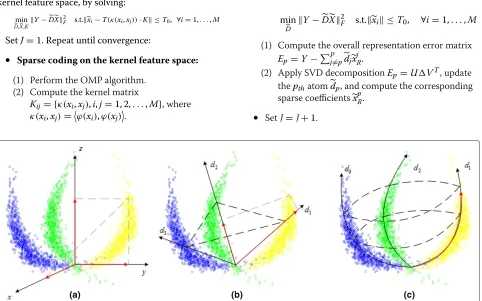
In the kernel methods, the dimension of a kernel matrix is determined by the number of training samples instead of the dimension of input samples. Hence, the kernel func-tion enables efficient operafunc-tions on a high-dimensional linear space and avoids ‘dimension disaster’ in the tradi-tional pattern analysis algorithms. As a result, the pro-posed Kernel KSVD approach deals with nonlinearity without having to know the concrete form of the nonlin-ear mapping function. As shown in Figure 2, we analyzed the target decomposition performance based on (a) scat-tering mechanisms, (b) KSVD and (c) Kernel KSVD.

Figure 1General model of kernel methods.

feature space where PCA is used to establish a linear rela-tionship. The kernel function used in KPCA is GRBF, and the corresponding feature space becomes a Hilbert space of infinite dimension. As shown in Figure 3, we will perform the proposed algorithm on three polarimetric matrixes, namely scattering matrix [S], covariance matrix [C] and coherency matrix [T], to generate the respective sparse codes. The codes of each matrix is pooled by Spatial Pyramid Machine (SPM) [16], and a linear SVM classifier [17] is finally used to give classification accuracy.

Task: Find the nonlinear dictionary and sparse compo-sitions to represent the data samplesY ∈ RN×M in the kernel feature space, by solving:

min D,X,KY−

DX2F s.t.xi−T(κ(xi,xj))·K ≤T0, ∀i=1,. . .,M

SetJ=1. Repeat until convergence:

• Sparse coding on the kernel feature space:

(1) Perform the OMP algorithm. (2) Compute the kernel matrix

Kij= {κ(xi,xj),i,j=1, 2,. . .,M}, where

κ(xi,xj)=

ϕ(xi),ϕ(xj)

.

(3) Compute the Eigenvalue component of the kernel matrixKα=λα, whereλis the Eigenvalue of the matrix, andαis the corresponding Eigenvector. (4) Normalize the Eigenvectorα_iTαi= λ1; all

Eigenvalues are sorted in descending order;λis the minimum non-zero Eigenvalue of matrixK. (5) Extract the principal component of test point

xp=Mj=1αp,jK(xi,xj),p=1,. . .,P, whereαk,jis

thejthelement of the Eigenvector, and generate

the sparse matrixX=[x1,x2,. . .,xM].

• Dictionary update:For each atomdp, update it by

min

D

Y−DX2_F s.t.xi ≤T0, ∀i=1,. . .,M

(1) Compute the overall representation error matrix Ep=Y−Pj =pdjxjR.

(2) Apply SVD decompositionEp=UVT, update

thepthatomdp, and compute the corresponding

sparse coefficientsxp_R. • SetJ=J+1.

Figure 2Decomposition performance based on scattering mechanisms, KSVD and Kernel KSVD.The blue, green and yellow points represent the nonlinear feature in the input space. Thex,y,zis some fixed coordinate system based on scattering me chanisms andd1,d2,d3is the learned

coordinate system based on KSVD and Kernel KSVD algorithm. The red arrows represent the projections of the yellow points on different decomposition bases.(a)Decomposition based on scattering mechanisms,x,y,zis orthogonal.(b)Decomposition based on KSVD algorithm, d1,d2,d3is linear towards the direction of feature points.(c)Decomposition based on proposed the Kernel KSVD algorithm,d1,d2,d3is a

Figure 3Framework of learning-based target decomposition method using Kernel KSVD algorithm.

Experiment Experimental setup

Two sets of experimental data adopted were derived from the airborne X-Band single-track PolSAR provided by the 38th Institute of China Electronics Technology Company.

Rice data

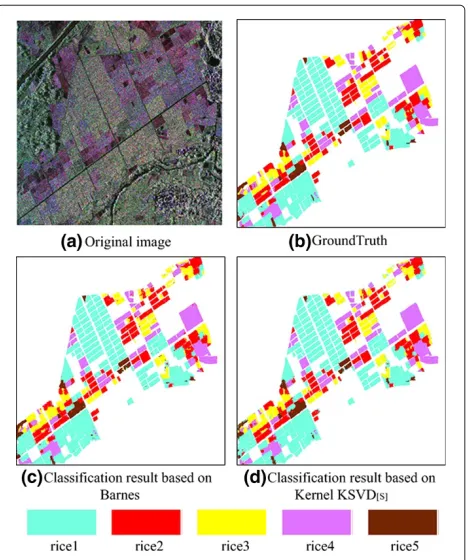
The photograph (Figure 4a) is an image of rice field of Lingshui County, Hainan Province, China. The original picture is 2, 048 × 2, 048 pixels and 1 × 1 resolution. We manually labeled the corresponding ground-truth image (Figure 4b) using ArcGIS software with five classes, namelyrice1,rice2,rice3,rice4 andrice5, according to dif-ferent growth periods after investigation by the author. In our experiment, we sampled the data in 683 × 683 pixels.

Orchard data

The photograph (Figure 5a) is an image of an orchard of Lingshui County, Hainan Province, China. The origi-nal piture is 2, 200×2, 400 pixels. The ground objects we are interested in aremango1,mango2,mango3,betelnut

andlongan, which are identified by different colors in the labeling image (Figure 5b). The three different types of mango represent different growth periods. In our experi-ment, we sampled the data in 440×480 pixels.

Experimental process

The proposed learning-based algorithm aims to perform Kernel KSVD decomposition on the scattering matrix [S],

Figure 4Experimental results of rice dataset.(a)Original image; (b)Ground truth;(c)Classification results based on Barnes decomposition;(d)Classification results based on Kernel KSVD[S]

Figure 5Experimental results of orchard dataset.(a)Original image;(b)Ground truth;(c)Classification results based on FourComponent decomposition;(d)Classification results based on Kernel KSVD[S]decomposition.

covariance matrix [C] and coherency matrix [T]. In gen-eral, the scattering intensity of four different channels, namelyHH, HV, VH andVV, is treated as the compo-nent of scattering matrix [S]. When the reciprocity theory ensures scattering intensity ofHV channel equals that of

VH, we can represent the scattering matrix of each pixel as a three-dimensional vector. Covariance matrix [C] and coherency matrix [T] can also be represented as a nine-dimensional matrix under the reciprocity theory. In this article, we only take the amplitude information of the matrix [S], [C] and [T] into consideration owing to the complication of the proposed decomposition method.

In the experiment, we first treat each pixel of the image as a vector made of three or nine elements, based on which the proposed Kernel KSVD algorithm performs decom-position and generates an over-complete dictionary of certain size. Then, we combine the sparse codes with spa-tial information using a three-level SPM to get the final spatial pyramid features of the image. Finally, a simple linear SVM classifier is used to test the classification per-formance. The grid size of SPM is 1×1, 2×2 and 4×4. In each region of the spatial pyramid, the sparse codes are pooled together to form a new feature. There are three kinds of pooling methods, namely the max pooling (Max) [18], the square root of mean squared statistics (Sqrt), and

the mean of absolute values (Abs). Due to the presence of speckle noise in the SAR image, this article chooses Abs as the pooling function.

Max : u=max(x1,x2. . .,xM)

Sqrt : u=

1 M

M

i=1xi

Abs : u= _M1

M

i=1 |xi|

The proposed Kernel KSVD algorithm is a nonlinear extension of KSVD algorithm by introducing a kernel method between sparse coding and atom updating stages. We choose the KPCA approach using Gaussian kernel function as our method. The covariance of kernel func-tion is 0.5 and the training ratio in KPCA is 10% of sparse coefficient matrix. All the experiments are averaged over a ratio of 10% training and 90% testing in linear SVM.

Comparison experiment

To illustrate the efficiency of Kernel KSVD algorithm, we devised a comparison experiment of SAR target decompo-sitions based on different scattering mechanisms, includ-ing the Pauli, the Krogager, the Cameron, the Freeman, the Four-Component, the OEC, the Barnes, the Holm, the Huynen and the Cloude decompositions. In the compar-ison experiment, the decomposition coefficients of each polarimetric matrix are processed with SPM and a linear SVM classifier is also used to generate the classifica-tion result. The comparison features of Kernel KSVD and other physical decompositions are shown in Table 1.

Experimental results

Experimental results on rice data

We followed the common experiment setup for rice data. Table 2 gives the detailed comparison results of target decomposition based on Kernel KSVD and other scat-tering mechanisms under different polarimetric matrixes. Figure 4c,d shows the classification results based on Barnes and Kernel KSVD[S]decomposition. As shown in Table 2, for matrix [S], the improvements in Kernel KSVD are 20.9, 3.6 and 1.5% than other three traditional decom-positions. For matrix [C], Kernel KSVD cannot achieve a higher classification result than the FourComponent and the Freeman decompositions, particularly for rice2 and

Table 1 Comparison features

Matrix Matrix [S] Matrix [C] Matrix[T]

Pauli(3) Freeman(3) Barnes(3)

Krogager(3) FourComponent(4) Holm(3)

Feature(Dim) Cameron(3) OEC(3) Huynen(3)

Cloude(3)

Kernel KSVD[S](5)

Kernel KSVD[C](10)

Table 2 Classification accuracy of Kernel KSVD and other decomposition methods based on different polarimetric matrixes for rice data (the bolded value represents the maximum accuracy among Kernel KSVD and the responding comparison methods for each ground object and each polarimetric matrix)

Matrix Feature rice1 rice2 rice3 rice4 rice5 Accuracy

Kernel KSVD[S] 98.64 94.08 95.05 95.65 90.76 96.49

Coherency 89.95 53.76 65.95 66.05 71.73 75.55

Matrix [S] Krogager 96.73 91.31 89.76 89.64 85.34 92.91

Pauli 98.35 92.02 92.09 93.07 90.18 95.02

Kernel KSVD[C] 98.67 90.09 91.01 92.55 86.91 94.48

OEC 96.27 93.42 89.62 87.11 86.58 92.53

Matrix [C] FourComponent 97.87 94.37 93.76 93.73 90.12 95.55

Freeman 97.90 92.37 92.39 93.22 90.66 94.97

Kernel KSVD[T] 98.90 92.47 92.47 94.19 87.01 95.78

Cloude 94.16 84.43 84.29 84.63 69.29 88.24

Matrix [T] Huynen 97.26 90.63 90.93 91.82 88.89 93.85

Holm 96.97 92.14 90.88 90.83 82.34 93.44

Barnes 98.37 94.06 94.06 95.40 90.56 96.13

rice5. For matrix [T], the classification accuracy of Kernel KSVD is 0.4% lower than the Barnes decomposition.

Experimental results on orchard data

We also tested our algorithm on orchard data. Table 3 demonstrates the classification accuracies based on Ker-nel KSVD and scattering mechanisms under different matrixes, and Figure 5c,d shows the classification results based on FourComponent and Kernel KSVD[S] decom-position. From Table 3, the decomposition based on Ker-nel KSVD again achieves much better performance than decompositions based on scattering mechanisms under

matrix [S], [C] and [T], respectively. Compared with the best physical decomposition on each polarimetric matrix, improvements in Kernel KSVD are 7.3, 7.6 and 6.1%, respectively. From Tables 2 and 3, we find that Coherency and Cloude decompositions are not able to achieve a sat-isfactory classification for both sets of data. The reason may be that the responding scattering mechanisms are not associated with categories in rice and orchard data. As we can see, it is necessary to take such an association into account in traditional decompositions. However, Kernel KSVD can always show an acceptable accuracy for differ-ent ground objects without considering this relationship

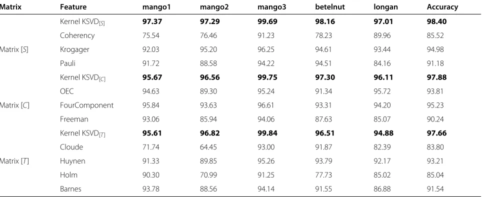
Table 3 Classification accuracy of Kernel KSVD and other decomposition methods based on different polarimetric matrixes of orchard data (the bolded value represents the maximum accuracy among Kernel KSVD and the responding comparison methods for each ground object and each polarimetric matrix)

Matrix Feature mango1 mango2 mango3 betelnut longan Accuracy

Kernel KSVD[S] 97.37 97.29 99.69 98.16 97.01 98.40

Coherency 75.54 76.46 91.23 78.23 89.96 85.52

Matrix [S] Krogager 92.03 95.20 96.25 94.61 93.44 94.98

Pauli 91.72 88.58 94.22 94.51 84.16 91.18

Kernel KSVD[C] 95.67 96.56 99.75 97.30 96.11 97.88

OEC 94.63 89.30 95.24 91.34 95.72 93.81

Matrix [C] FourComponent 95.84 93.63 96.61 93.31 94.20 95.23

Freeman 93.06 85.94 94.06 87.63 85.07 90.24

Kernel KSVD[T] 95.61 96.82 99.84 96.51 94.88 97.66

Cloude 71.74 64.45 93.00 91.87 82.39 83.80

Matrix [T] Huynen 91.33 89.85 95.26 93.79 92.17 93.21

Holm 90.30 70.99 91.25 77.73 85.02 85.04

due to its adaptive learning-based method. In addition, we can also find that the classification based on the proposed algorithm can achieve better results on matrix [S] than matrix [C] and [T].

Conclusion

This article presents a learning-based target decomposi-tion method based on the Kernel KSVD model for the classification of SAR images. Experimental results on the two sets of SAR data indicate that the proposed method has better performance than traditional decompositions based on scattering mechanisms in the classification of SAR images.

The success of the proposed kernel KSVD algorithm is largely due to the following reasons: first, Kernel KSVD is an extension of KSVD method with inheritance of adap-tive characteristics for dictionary learning; second, KPCA is used to capture nonlinearity via projecting the sparse coefficients into a kernel feature space, in which the zero coefficients will be eliminated through inner product. finally, Kernel KSVD constructs a curvilinear coordinate for target decomposition that goes along the flow of non-linear feature points. We will further apply this method for different land covers classification as a future work.

Competing interests

The authors declare that they have no competing interests.

Acknowledgements

This study was supported by the National Basic Research Program of China (973 program) under Grant No. 2011CB707102, NSFC grant (No. 60702041, 41174120), the China Postdoctoral Science Foundation funded project and the LIESMARS Special Research Funding.

Received: 5 January 2012 Accepted: 15 May 2012 Published: 24 July 2012

References

1. H Maitre,Traitement des Images de Radar `a Synth`ese d’Ouverture(Herm`es Science Publication, Lavoisier, 2001)

2. E Pottier, J Saillard, On radar polarization target decomposition theorems with application to target classification by using network method. in Proceedings of the International Conference on Antennas and Propagation, vol. 1,(York, England, 1991), pp. 265–268

3. DH Hoekman, MAM Vissers, TN Tran, Unsupervised full-polarimetric SAR data segmentation as a tool for classification of agricultural areas. IEEE J. Sel. Top. Appl. Earth Obser. Remote Sens.4(2), 402–411 (2011)

4. H Skriver, F Mattia, G Satalino, A Balenzano, VRN Pauwels, NEC Verhoest, M Davidson, Crop classification using short-revisit multitemporal SAR data. IEEE J. Sel. Top. Appl. Earth Obser. Remote Sens.4(2), 423–431 (2011) 5. Y Yamaguchi, Y Yajima, H Yamada, A four-component decomposition of

PolSAR images based on the Coherency matrix. IEEE Geosci. Remote Sens. Lett.2(2), 292–296 (2006)

6. H Lee, A Battle, R Raina, A Ng, Efficient sparse coding algorithms. in

Proceedings of the Neural Information Processing Systems,(Vancouver, B. C.,

Canada, 2006), pp. 4–9

7. M Aharon, M Elad, A Bruckstein,K-SVD: an algorithm for designing of overcomplete dictionaries for sparse representation. IEEE Trans. Signal Process.54(11), 4311–4322 (2006)

8. L Bottou,Online Learning and and Stochastic Approximations. Online

Learning in Neural Networks(Cambridge University Press, Cambridge,

1998), pp. 9–42

9. B Scholkopf, S Mika, CJC Burges, P Knirsch, KR Muller, G Ratsch, AJ Smola, Input space versus feature space in kernel-based methods. IEEE Trans. Neural Netw.10(5), 1000–1017 (1999)

10. A Smola, B Scholkopf, KR Muller, Nonlinear component analysis as a Kernel eigenvalue problem. Neural Comput.10(6), 1299–1319 (1998) 11. FR Bach, MI Jordan, Kernel independent component analysism. J. Mach.

Lear. Res.3, 1–48 (2002)

12. Q Liu, H Lu, S Ma, Improving kernel Fisher discriminant analysis for face recognition. IEEE Trans. Circ. Syst. Video Technol.14(1), 42–49 (2004) 13. FT Ulaby, C Elachi,Radar Polarimetry for Geoscience Applications(Artech

House, Norwood, 1990)

14. S Mallat, Z Zhang, Matching pursuits with time-frequency dictionaries. IEEE Trans. Signal Process.41(12), 3397–3415 (1993)

15. YC Pati, R Rezaiifar, PS Krishnaprasad, Orthogonal matching pursuit: recursive function approximation with applications to wavelet decomposition. inProceedings of Asilomar Conference on Signals, Systems

and Computers,vol. 1,(California, USA, 1993), pp. 40–44

16. S Lazebnik, C Schmid, J Ponce, Beyond bags of features: spatial pyramid matching for recognizing natural scene categories. inProceedings of the IEEE Computer Society Conference on Computer Vision and Pattern

Recognition,vol. 2,(New York, 2006), pp. 2169–2178

17. Chih-Chung Chang etc. LIBSVM: a library for support vector machines. Available: http://www.csie.ntu.edu.tw/cjlin/libsvm, 2011

18. J Yang, K Yu, Y Gong, T Huang, Linear spatial pyramid matching using sparse coding for image classification. inProceedings of the IEEE Computer

Society Conference on Computer Vision and Pattern Recognition,(Miami,

2009), pp. 1794–1801

doi:10.1186/1687-6180-2012-159

Cite this article as: He et al.: A learning-based target decomposition

method using Kernel KSVD for polarimetric SAR image classification. EURASIP Journal on Advances in Signal Processing20122012:159.

Submit your manuscript to a

journal and benefi t from:

7Convenient online submission 7Rigorous peer review

7Immediate publication on acceptance 7Open access: articles freely available online 7High visibility within the fi eld

7Retaining the copyright to your article