Volume 2010, Article ID 375171,6pages doi:10.1155/2010/375171
Research Article
Attenuation Analysis of Lamb Waves Using
the Chirplet Transform
Florian Kerber,
1Helge Sprenger,
2Marc Niethammer,
3Kritsakorn Luangvilai,
4and Laurence J. Jacobs
41Institute of Mathematics and Computing Science, University of Groningen, 9700 AV Groningen, The Netherlands 2Institute of Applied and Experimental Mechanics, University of Stuttgart, Pfaffenwaldring 9, 70569 Stuttgart, Germany 3Computer Science Department, University of North Carolina, Chapel Hill, NC 27599-3175, USA
4School of Civil and Environmental Engineering and G.W. WoodruffSchool of Mechanical Engineering, Georgia Institute of Technology,
Atlanta, GA 30332, USA
Correspondence should be addressed to Florian Kerber,[email protected]
Received 22 December 2009; Revised 26 March 2010; Accepted 10 June 2010
Academic Editor: Jo˜ao Marcos A. Rebello
Copyright © 2010 Florian Kerber et al. This is an open access article distributed under the Creative Commons Attribution License, which permits unrestricted use, distribution, and reproduction in any medium, provided the original work is properly cited.
Guided Lamb waves are commonly used in nondestructive evaluation to monitor plate-like structures or to characterize properties of composite or layered materials. However, the dispersive propagation and multimode excitability of Lamb waves complicate their analysis. Advanced signal processing techniques are therefore required to resolve both the time and frequency content of the time-domain wave signals. The chirplet transform (CT) has been introduced as a generalized time-frequency representation (TFR) incorporating more flexibility to adjust the window function to the group delay of the signal when compared to the more classical short-time Fourier transform (STFT). Exploiting this additional degree of freedom, this paper applies an adaptive algorithm based on the CT to calculate mode displacement ratios and attenuation of Lamb waves in elastic plate structures. The CT-based algorithm has a clear performance advantage when calculating mode displacement ratios and attenuation for numerically-simulated Lamb wave signals. For experimental data, the CT retains an advantage over the STFT although measurement noise and parameter uncertainties lead to larger overall deviations from the theoretically expected solutions.
1. Introduction
Ultrasonic waves are often used in nondestructive testing to evaluate the integrity of structural components, as well as to determine material properties of composite or layered materials. In various disciplines such as civil or aerospace engineering, multimode, dispersive guided waves such as Lamb waves have been applied, see Chimenti [1] for an overview. However, complicated signal analysis is the trade off for their versatility. In fact, the main challenges to process Lamb wave signals are due to their very characteristics. Firstly, dispersion phenomena require a resolution of the frequency content of a Lamb wave signal over time which is inherently compromised by the uncertainty principle. Secondly, Lamb waves are multi-modal, which means that interferences between individual modes complicate the allocation of energy and displacement
be used to localize notches in plates by means of a correlation technique, see [5]. Ultrasonic attenuation describes the amplitude decay of wave modes due to energy leakage or the geometry of a specimen. Geometric spreading of Lamb waves in plate structures was examined by Luangvilai et al. [6] using the STFT. Energy leakage in absorbing plates was studied by Luangvilai et al. [7] to determine attenuation coefficients using a refined STFT algorithm. While STFT-based techniques analyze multimode time-domain signals as a whole, the CT-based algorithm uses basis functions specially adjusted to the dispersion relation of each mode of propagation. Physical quantities like displacement or energy can thus be allocated more consistently to individual modes. Since the shaping of the basis functions depends on the knowledge of the dispersion relation for a given set-up, this work considers both numerically simulated ([6]) and experimentally generated ([5]) time-domain signals of Lamb waves in an aluminum plate to evaluate the robustness of the CT-based algorithm as well as its performance.
The paper is organized as follows: first a general def-inition of the CT is given before describing its use in NDE applications to resolve the time-frequency content of dispersive wave signals by means of an adaptive model-based algorithm.Section 3contains a description of the candidate NDE problem. The results for mode displacement ratios and geometric spreading of both theoretically and experimentally generated wave signals are presented in Section 4. The concluding remarks ofSection 5outline possibilities to apply the presented technique to other NDE applications.
2. The Chirplet Transform and Its Use in
Dispersive Wave Analysis
The chirplet transform has been introduced as a generalized time-frequency representation by Mann and Haykin [8]. The basis function can be adjusted by means of shift, shear, and scaling operators, resulting in a five-dimensional parameter space for the energy density which comprises as projections the respective densities obtained from a short-time Fourier transform (short-time and frequency shift) and a wavelet transform (time shift and scaling).
2.1. Definition of the Chirplet Transform. The standard
definition of the chirplet transform is given by the inner product of a basis functiong(t) and the signalx(t),
Cctt
0,ω0,s,q,p
= ∞
−∞x(t)g ∗
t0,ω0,s,q,p(t)dt
= 1 2π
∞
−∞X(ω)G ∗
t0,ω0,s,q,p(ω)dω,
(1)
where ∗ denotes complex conjugation. The basis function
g(t) as well as its Fourier transformG(ω) belongs to a family of chirp signals,
Gt0,ω0,s,q,p(ω)=Tt0Fω0SsQqPpH(ω),
gt0,ω0,s,q,p(t)=Tt0Fω0SsQqPph(t),
(2)
where the operators Tt0,Fω0,Ss,Qq, and Pp act in the
following manner on the window functionh(t) or its Fourier transformH(ω), respectively,
Time shift:
Tt0h(t)=h(t−t0), Tt0H(ω)=e
−iωt0H(ω). (3)
Frequency shift:
Fω0h(t)=e
iω0th(t), F
ω0H(ω)=H(ω−ω0). (4)
Scaling:
Ssh(t)= 1 √
sh(t/s), SsG(ω)=
√
sG(sω). (5)
Time shear:
Pph(t)=
ip−1/2exp
it
2
2p
h(t),
PpH(ω)=exp
ip
2ω 2
H(ω).
(6)
Frequency shear:
Qqh(t)=exp
iq
2t 2
h(t),
QqH(ω)=(iq)−1/2exp
i2ω
2
q H(ω)
.
(7)
Higher order time shear Pp1,p2,...H(ω) can also be applied
resulting in
Pp1,p2,...H(ω)=exp
i p1
2ω 2+ p2
3 ω 3+· · ·
H(ω), (8)
and similarly, higher order frequency shear is given by
Qq1,q2,...h(t)=exp
i q1
2t 2+q2
3t 3+· · ·
h(t). (9)
The energy density Pct of the chirplet transform at every point (t0,ω0,s,q,p) in the five dimensional parameter space is given by
Pctt0,ω0,s,q,p
=Cctt0,ω0,s,q,p2. (10) By comparison, the short-time Fourier transform only allows to shift the window function in time and frequency,
Gt0,ω0(ω)=Tt0Fω0H(ω), gt0,ω0(t)=Tt0Fω0h(t), (11)
to obtain
Cstft(t0,ω0)= ∞
−∞x(t)g ∗
t0,ω0(t)dt
= 1 2π
∞
−∞X(ω)G ∗
t0,ω0(ω)dω.
(12)
The energy density of the STFT, the spectrogram, is given by
Pstft(t
0,ω0)=Cstft(t0,ω0) 2
. (13)
2.2. Adaptive Algorithm Based on the Chirplet Transform. For ease of visualization, only subspaces of the five-dimensional parameter space of the chirplet transform are considered. In a fashion analogous to the STFT and its energy den-sity representation, the spectrogram, the time-frequency plane is chosen to analyze dispersive waves. According to the definition of the energy density Pi,i ∈ {stft, ct}, the squared amplitude of a time-domain signal recording particle displacement is proportional to the energy of the incident Lamb wave, but comprises contributions of all modes of propagation. The objective is to identify energy or displacement related components of individual modes in regions of sufficient mode separation. To that end, the energy content of the time-domain signal is averaged in the time-frequency plane over a region around every point of the dispersion curve of a particular mode using a specially designed window function. In the case of the STFT, time and frequency shift operations result in a region of averaging that approximates the group delay of an individual mode of propagation with zeroth order, whereas the CT-based algorithm as described by Kuttig et al. [4] additionally uses time shearing resulting in higher order approximations. Note that the dispersion curves for a given system depend on the material properties—in the example of a single aluminum plate, its elastic modulus and density as well as its thickness— which determines the robustness of the CT-based algorithm. For this research, the CT is calculated with a normalized Gaussian window
g(t)= 1
4
πs2 0
exp
−1 2
t−t0
s0 2
, (14)
with a default value ofs0 =2.2μs. ScalingSsis 1 by default unless the 3σ-isopleths of (14) described by ellipses with half-axis of 3s0in time and 1/(3s0) in frequency intersect with the dispersion curve of another mode. Thus, at least 99.9% of the energy of the window function is concentrated around the mode of interest. The dispersion curves are approximated by a fifth-order polynomial around every point (t0,ω0),
t(ω)=t0+p1(ω−ω0) +p2(ω−ω0)2+· · ·+p5(ω−ω0)5. (15)
The group delayτg(ω) of a signalH(ω)=A(ω) exp[iφ(ω)] in frequency domain is given by
τg(ω)= − d
dωφ(ω). (16)
The group delay of the window functionGt0,ω0,p1,p2,...,p5(ω)=
Tt0Fω0Pp1,p2,...,p5H(ω) can thus be fitted to (15) for every
mode of propagation by a fifth-order time shear (8) with parameters p1,. . .,p5. Figure 1 depicts the 3σ-regions of window functions adjusted by the adaptive algorithm for the first symmetrical mode s0. The CT is not calculated in frequency regions of interference with other modes, for example, around 2 MHz at the intersection of the a0- and
s0-mode. More details about the adaptive algorithm can be found in [4]. The same Gaussian window function (14) was also used for the STFT-based analysis.
100 200 300 400 500 600 700 800
Ti
m
e
(
μ
s)
0 1 2 3 4 5 6 7 8 9 10
Frequency (MHz)
a0
a1
s0
s1
s2
a2
a3
a4
s4
s3
Figure1: CT basis functions adjusted to the s0-mode using 5th-order time shear. The dispersion curves are the solution of the
Rayleigh-Lamb equations (17) for an aluminum 3003 plate of
thickness 0.99 mm and source-receiver distance of 90 mm.
3. Problem Setting
In this paper, Lamb waves traveling in aluminum plate structures are considered. Due to the relatively simple geometry of the plate, it is possible to compute dispersion curves based on the analysis of the Rayleigh-Lamb equations for stress-free boundaries as derived in Achenbach [9],
tanqh
tanph = −
4k2pq
q2−k22,
tanqh
tanph = −
q2−k22 4k2pq ,
(17)
where
p2=ω2
c2 L
−k2, q2=ω2
c2 T
−k2, (18)
Displacement ratioa0/s0
0 0.1 0.2 0.3 0.4 0.5 0.6 0.7 0.8 0.9 1
N
o
rm
aliz
ed
mode
displac
ement
0 1 2 3 4 5 6 7 8 9 10
Frequency (MHz) Theoretical
STFT CT
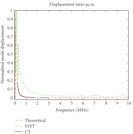
Figure2: Out-of-plane displacement ratio of modes0normalized
to modea0for the synthetic signal.
an aluminum plate of dimensions 100 mm × 100 mm × 1 mm and a noncontact, point-like laser measurement and detection system. A laser source was used to generate Lamb waves in the aluminum plate for different source-receiver distances ranging from 50 to 150 mm.
For each of the two data sets, the mode displacement ratios for selective modes are determined as a means to detect material irregularities, for example, for notch localization as in [5]. Apart from that, the amplitude decay over time of individual modes is analyzed as it contains information about the geometry of the specimen. Geometric spreading is given by the quotientd2/d1for two propagation distances
d1< d2. Such a normalized measure for geometric spreading is chosen since the effect of the excitation source on the energy density will be canceled out.
4. Results
First consider the results obtained for the numerically simulated signal. The particle displacement associated to a particular mode is extracted from the modulus|Ci(t
0,ω0)|,
i∈ {stft, ct}of each transform. To eliminate the effect of the excitation source, these values are normalized to a particular mode—Table 1 contains the results for normalization with respect toa0ands0—by taking the point-by-point quotient of the respective moduli at every frequency ω0. Figure 2 shows the ratios0/a0 as obtained from the STFT- and CT-based algorithm versus the exact theoretical solution. The latter are very close to the theoretical solution, while the amplitude ratio extracted from the STFT deviates especially at frequencies where individual modes are highly dispersive such as thes0-mode for frequencies between 2 and 3 MHz. Since the STFT does not use window functions adjusted to
CT-based results for modea0
1.1 1.2 1.3 1.4 1.5
Geomet
ri
c
spr
eading
d
2
/d1
0.5 1 1.5 2 2.5
Frequency (MHz) (a)
CT-based results for modea0
1 1.2 1.4 1.6 1.8 2 2.2
Geomet
ri
c
spr
eading
d
2
/d1
0.5 1 1.5 2 2.5
Frequency (MHz) (b)
Figure3: Geometric attenuation for thea0-mode of the synthet-ically generated signal determined with the STFT (b) and CT (a).
Dashed lines represent the theoretically expected solutiond2/d1,
dash-dotted lines are the results obtained from the CT- and STFT-based algorithm, respectively, for the distances 40 mm (pink), 50 mm (green), 60 mm (black), 70 mm (blue), and 80 mm (red) related to 90 mm of propagation distance.
the dispersion behavior of individual modes, drastic changes in the group delay can lead to inconsistent values using the STFT, whereas the CT can keep a high level of accuracy.
In order to quantify the level of accuracy of each method, a simple metricpis introduced that maps a functionx(t) on a positive real number,
x(t)−→p(x(t))=
x(t),x(t)
L , (19)
whereL=−∞∞ dtand·,· is defined as the inner product for functions [10],x(t),y(t) = −∞∞ x∗(t)y(t)dt. This metric will be used to measure the mean absolute deviation of quantities extracted with the introduced signal processing techniques from the theoretical solution. Note that the adaptive CT-based algorithm only computes energy densities in frequency regions where individual modes are sufficiently separated, that is, when the 3σ-region of averaging does not intersect with any other mode. The performance measure for both the STFT- and the CT-based method will therefore be restricted to these regions only.Table 1confirms that the CT-based results for the numerically simulated signal deviates much less from the theoretical solution compared to the ones obtained from the STFT.
Table1: Average deviation from theoretical mode displacement ratio in %.
displacement ratio a1/a0 s0/a0 s1/a0 a0/s0 a1/s0 s1/s0
numerical signal CT (in %) 9.49 67.89 8.46 10.54 4.00 12.19
STFT (in %) 18.60 686.36 14.65 51.33 66.28 10.24
experimental signal CT (in %) 173.73 46.96 343.88 35.75 272.29 484.40
STFT (in %) 115.36 83.06 223.07 52.99 289.76 385.70
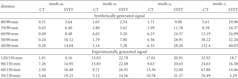
Table2: Average deviation in % from theoretical geometric attenuation.
distance modea0 modea1 modes0 modes1
CT STFT CT STFT CT STFT CT STFT
Synthetically generated signal
80/90 mm 0.31 3.64 1.65 2.54 1.71 9.08 5.61 19.96
70/90 mm 0.43 6.40 2.80 3.62 1.99 11.78 8.39 24.37
60/90 mm 0.49 8.48 4.65 5.20 6.23 24.37 13.19 24.09
50/90 mm 0.24 10.12 1.79 7.80 6.56 28.91 38.22 32.26
40/90 mm 0.28 14.04 3.14 7.28 6.33 28.26 132.4 40.03
Experimentally generated signal
120/150 mm 1.91 4.16 15.03 22.78 17.01 20.91 32.92 18.7
90/150 mm 7.26 14.95 15.83 22.08 9.63 20.63 24.63 16.38
60/150 mm 2.50 16.48 9.71 26.91 13.56 32.68 67.88 14.46
50/150 mm 3.44 19.21 3.12 14.56 10.78 31.37 76.49 5.29
expected ratiod2/d1for different source receiver distances normalized to the longest distance 90 mm. The theoreti-cal solution is compared to the quotient of the moduli |Ci(t
0,ω0)|, i ∈ {stft, ct} which represent the amplitudes calculated at a frequencyω0for a particluar mode. The CT-based algorithm almost exactly predicts geometric spreading over the frequency range from about 0.3 to 1.5 MHz. In contrast, the STFT results differ from the theoretically expected amplitude decay even in those regions where the
a0-mode is separated. This is confirmed by earlier results of Luangvilai et al. [6] who reported that the amplitude decay due to the propagation pattern cannot be recalculated exactly using the spectrogram. A similar observation can be made for modesa1,s0, ands1as well, that is, the relative error for the CT is up to ten times smaller than the STFT results, c. f.
Table 2. Only in frequency regions in which the group delay
is almost constant, for example, at about 1-2 MHz for thea0 -mode, both transforms produce similar amplitude ratios. In general, longer propagation distances improve the resolution due to better mode separation in the time-frequency plane.
The analysis of the experimentally obtained data yields smaller differences between the two methods as shown by the mean relative deviations from the exact solution for both the mode displacement ratios and geometric spreading, see Tables 1 and2. The CT produces results closer to the theoretically expected solution, especially if source-receiver distances are large enough as can be seen inFigure 4when comparing geometric spreading for propagation distances of 50 mm (green curve) and 120 mm (red curve) relative to 150 mm. However, the level of accuracy drops considerably compared to the previous results. The extraction of both displacement and energy related quantities associated with
individual modes from a time-frequency representation depends on the dispersion relation, which in turn is deter-mined by the material properties of the specimen. Parameter variations as well as measurement noise therefore influence the accuracy of the STFT-based approach and even more the CT-based algorithm since in the latter case, the basis functions are adjusted for the dispersion, too. When the theoretical dispersion curves are closely matched as for the numerically simulated signal, the performance advantage of the CT-based algorithm becomes apparent.
5. Conclusions
CT-based results for modea0
0.8 1 1.2 1.4 1.6 1.8
Geomet
ri
c
spr
eading
d
2
/d1
0.5 1 1.5 2 2.5 3 3.5 4 Frequency (MHz)
(a)
CT-based results for modea0
1.2 1.4 1.6 1.8 2 2.2 2.4 2.6 2.8
Geomet
ri
c
spr
eading
d
2
/d1
0.5 1 1.5 2 2.5 3 3.5 4 Frequency (MHz)
(b)
Figure4: Geometric attenuation for thea0-mode of the experimen-tally generated signal determined with the STFT (b) and CT (a).
Dashed lines represent the theoretically expected solutiond2/d1,
dash-dotted lines are the results obtained from the CT- and STFT-based algorithm, respectively, for the distances 50 mm (green), 60 mm (black), 90 mm (blue), and 120 mm (red) related to 150 mm of propagation distance.
Since the dispersion relation in turn depends on the material properties and geometry of the specimen, precise knowledge about experimental set-up is a prerequisite to obtain reliable results with this technique. Consequently, the level of accuracy is considerably lower when applied to the experimentally generated data, also for the STFT-based approach. Improving robustness properties as well as algorithmic efficiency remains a goal of future research to make the CT-based technique more easily available and applicable for quantitative nondestructive evaluation.
Acknowledgment
The Deutscher Akademischer Austausch Dienst (DAAD) provided partial support to F. Kerber.
References
[1] D. E. Chimenti, “Guided waves in plates and their use in
materials characterization,” Applied Mechanics Reviews, vol.
50, no. 5, pp. 247–284, 1997.
[2] M. Niethammer, L. J. Jacobs, J. Qu, and J. Jarzynski,
“Time-frequency representations of Lamb waves,”Journal of
the Acoustical Society of America, vol. 109, no. 5, pp. 1841– 1847, 2001.
[3] J.-C. Hong, K. H. Sun, and Y. Y. Kim, “Dispersion-based short-time Fourier transform applied to dispersive wave analysis,”
Journal of the Acoustical Society of America, vol. 117, no. 5, pp. 2949–2960, 2005.
[4] H. Kuttig, M. Niethammer, S. Hurlebaus, and L. J. Jacobs, “Model-based signal processing of dispersive waves with
chirplets,”Journal of the Acoustical Society of America, vol. 119,
no. 4, pp. 2122–2130, 2006.
[5] R. Benz, M. Niethammer, S. Hurlebaus, and L. J. Jacobs,
“Localization of notches with Lamb waves,” Journal of the
Acoustical Society of America, vol. 114, no. 2, pp. 677–685, 2003.
[6] K. Luangvilai, L. J. Jacobs, and J. Qu, “Far-field decay of
laser-generated, axisymmetric Lamb waves,” inReview of Progress in
Quantitative Nondestructive Evaluation, D. O. Thompson and
D. E. Chimenti, Eds., vol. 700 ofAIP Conference Proceedings,
pp. 158–164, 2003.
[7] K. Luangvilai, L. J. Jacobs, P. D. Wilcox, M. J. S. Lowe, and J. Qu, “Broadband measurement for an absorbing plate,” in
Review of Progress in Quantitative Nondestructive Evaluation,
D. O. Thompson and D. E. Chimenti, Eds., vol. 24 ofAIP
Conference Proceedings, pp. 297–304, 2005.
[8] S. Mann and S. Haykin, “The chirplet transform: a
generaliza-tion of Gabor’s logon transform,” inProceedings of the Vision
Interface, pp. 205–212, 1991.
[9] J. D. Achenbach,Wave Propagation in Elastic Solids, Elsevier,
New York, NY, USA, 1st edition, 1999.
[10] P. K. Jain, O. P. Ahuja, and K. Ahmed,Functional Analysis, John