University of Twente
EEMCS / Electrical Engineering
Control Engineering
Variable batch sizes for
Learning Feed Forward Control using Key
Sample Machines
Job Kamphuis
M.Sc. Thesis
Supervisors prof.dr.ir. J. van Amerongen
dr.ir. T.J.A. de Vries dr. ir. B.J. de Kruif
June 2005
Report nr. 024CE2005
Control Engineering EE-Math-CS
University of Twente P.O. Box 217
Function approximators are able to “learn” a function when presented with a set of training samples. The samples in this training set are generally corrupted by measurement noise. The function approximator will “filter out” this noise and is able to predict the function output value for a new input. Function approximators are used in feed forward controllers. Given a certain input e.g. the reference signal, it is possible to generate a control signal, which makes the physical system behave as dictated by the reference signal.
Function approximators as Least Squares Approximator or Support Vector Machine have been around for some time. During his PhD., dr. ir. B.J. de Kruif developed a new function approximator, which was capable of approximating certain functions that could not be approximated by other algorithms. Furthermore, this approximator, called Key Sample Machine (KSM) approximates the function in an efficient way, saving a lot of computer resources (De Kruif, 2004).
In this project the principals of the two existing variants of KSM are described in detail. The offline variant approximates the function in a non-recursive way. All samples in the training set are presented to the offline KSM at once. When the calculations are done, the offline KSM comes with a final approximation. The online variant approximates the function recursively and handles one training sample at a time. Both KSM algorithms were rebuilt in Matlab and each implementation step has been described in detail in this thesis.
During this project a new KSM algorithm has been developed. This key sample machine is able to handle samples in variable block sizes. It is therefore called “Blocked Key Sample Machine” (BKSM). The target function is approximated recursively, just as the online algorithm, but it can however handle more samples at a time. The handling of multiple samples is very similar to that of the offline key sample machine. The advantage of the BKSM compared to the online KSM is that the approximation is done quicker. Furthermore, the algorithm is contrary to the offline KSM, able to update the approximation continuously. This can be an asset or even a necessity for systems where the target function is not time invariant.
The BKSM algorithm has been tested in the simulation environment of 20-sim (Controllab Products b.v.). The plant is a model of a physical system, which is closely related to a printing device. A motor drives a belt on which a load mass is mounted. The position of the load has to be controlled. First the system is controlled by a PD-controller, which is later on extended with a BKSM feed forward controller. The maximum position error of the PD-controlled system is 2.54 10-3 [m]. When the controller is extended with the BKSM, the maximum position error of the system is 1.40 10-4 [m]. This means that the error decrease due to the BKSM is about 95 %.
Besides testing the BKSM in simulations, it was tested on a real physical system. This system is called “Mechatronic Demonstrator” (Dirne, 2005). As in the simulations, a PD-controller is used to control the system. This resulted in a maximum position error of 3.10 10-3 [m] and a maximum static position error of 3.00 10-4 [m]. After the controller was extended with the BKSM, the maximum position error decreased to a value of 4.30 10-4 [m]. This means that the maximum position error reduction is 85 %. The maximum static error was reduced by half to a value of 1.50 10-4 [m].
Samenvatting
Functieapproximators zijn in staat een functie te “leren” als er een traingset met samples wordt aangeboden. De samples in deze trainingset zijn over het algemeen besmet met meetruis. De functieapproximator “filtert” deze ruis en is in staat om de functiewaarde te voorspellen voor een gegeven inputwaarde. Functi approximators worden gebruikt in feed forward controllers. Met behulp van een input b.v. het referentiesignaal, is het mogelijk een stuursignaal te generen, waardoor het fysische systeem zich zal gedragen als door het referentiesignaal gedicteerd wordt.
Functieapproximators zoals Least Squares Approximators of Support Vector Machine worden al geruime tijd gebruikt. Tijdens zijn PhD., heeft dr. ir. B.J. de Kruif een nieuwe functieapproximator ontwikkeld, die in staat is om bepaalde functies te benaderen die niet te approximeren waren met behulp van andere algoritmen. Daarnaast approximeert deze functieapproximator, genaamd Key Sample Machine (KSM), functies in een efficiënte manier, waardoor er bespaard wordt op het gebruik van computer bronnen (De Kruif, 2004).
In dit project worden the principes achter the twee bestaande varianten van KSM in detail beschreven. The offline variant approximeert the functie in een niet-recursieve manier. Alle samples in de training set worden in één keer aangeboden aan de offline KSM. Als de berekeningen zijn gedaan, komt de offline KSM met een definitieve approximatie. De online variant approximeert de functie recursief en verwerkt de samples één voor één af. Beide KSM algoritmen zijn opnieuw geprogrammeerd in Matlab en elke stap in de implementatie is in detail beschreven in deze thesis.
Tijdens dit project een nieuw KSM algoritme is ontwikkeld. Deze key sample machine is in staat om samples in variabele blokgrootten te verwerken. Het wordt daarom “Blocked Key Sample Machine” (BKSM) genoemd. De doelfunctie wordt recursief geapproximeerd, zoals in het online algoritme, maar het kan echter meerdere samples tegelijkertijd verwerken. Het verwerken van meerdere samples lijkt erg op dat van de offline key sample machine. Het voordeel van de BKSM vergeleken met het online algoritme is dat de approximatie sneller wordt uitgevoerd. Daarbij is het algoritme in tegenstelling tot de offline KSM, in staat om de approximatie continu te updaten. Dit kan een nuttige eigenschap of zelfs een noodzaak zijn voor systemen waarvan de doelfunctie tijd variant is.
Het BKSM algoritme is getest in de simulatie omgeving van 20-sim (Controllab Products b.v.). Hiervoor wordt een model van een fysisch systeem gebruikt, dat sterk gerelateerd is aan een print machine. Een motor drijft een band aan waarop een massa is gemonteerd. De positie van de massa moet worden gestuurd. Eerst wordt het systeem aangestuurd door een PD-controller, die later wordt uitgebreid met een BKSM feed forward controller. De maximum positie fout van het door de PD-controller gestuurde systeem is 2,54 10-3 [m]. Als de controller wordt uitgebreid met de BKSM, wordt de maximale positie fout van het systeem 1,40 10-4 [m]. Dit betekent dat de fout verkleining ten gevolge van de BKSM ongeveer 95 % is.
Naast het testen van de BKSM in simulaties, is het getest op een fysisch systeem. Dit systeem wordt “Mechatronic Demonstrator” genoemd (Dirne, 2005). Zoals tijdens de simulaties, wordt eerst een PD-controller gebruikt om het systeem aan te sturen. Dit resulteert in een maximum positie fout van 3,10 10-3 [m] en een maximum statische positie fout van 3,00 10-4 [m]. Nadat de controller was uitgebreid met de BKSM, bedroeg de maximum positie fout 4,30 10-4 [m]. Dit betekent dat de maximum positie fout is gereduceerd met 85 %. De maximum statische positie fout is gereduceerd tot de helft met een waarde van 1.50 10-4 [m].
Preface
For years I have wished for the moment that my study Electrical Engineering, would come to an end. Now the moment is near, I feel ambivalent and tend to get emotional about it sometimes. There is so much I have learned during my time as a student. Of course I learned a lot about electrical engineering but I even learned a great deal more about myself. The first years have been pretty difficult and I have had several moments, I decided to stop studying electrical engineering. Therefore, the first people I would like to thank are my brother and especially my parents for their ever-lasting support. Second of all I would like to thank my best friend Hans Dirne. Although I would probably have finished this study three years earlier without him, his companionship was essential for having a good time while studying the tough and sometimes tedious subjects. Furthermore I would like to thank two housemates Victor van Eekelen and Joep ter Avest, for their contribution in making our home a great place to live and study.
I am grateful for the supervision of prof. dr. ir. J. van Amerongen and dr. ir. T.J.A. de Vries during this graduation project. They have been given me enough freedom to explore and demonstrate my capabilities as an engineer and also supported me well in the moments I needed some steering. I also would like to thank my third supervisor dr. ir. B.J. de Kruif for the hours he spent with me explaining the abstract mathematical procedures. He is also the main designer of the newly developed blocked key sample machine. I believe that without his help the scope of this project would have been limited severely.
Table of Contents
Summary ... i
Samenvatting ... ii
Preface... iii
1 Introduction ... 1
2 Least Squares function approximators... 3
2.1 Ordinary Least Squares function approximator ... 3
2.2 Dual Least Squares function approximator... 6
3 Existing Key Sample Machine algorithms ... 9
3.1 Offline Key Sample Machine ... 9
3.1.1 Training Set ... 11
3.1.2 Create potential indicators ... 12
3.1.3 Select indicator with maximum error reduction ... 13
3.1.4 Add key sample to existing set ... 15
3.1.5 Stop Criterion ... 20
3.1.6 Approximate the function... 21
3.1.7 Matlab Results ... 22
3.2 Online Key Sample Machine ... 23
3.2.1 Incoming sample ... 26
3.2.2 Kernel function... 26
3.2.3 Fine-tuning ... 26
3.2.4 Inclusion selection criterion ... 28
3.2.5 Inclusion of a key sample ... 29
3.2.6 Selection of potentially omitted key samples ... 31
3.2.7 Omission selection criterion ... 31
4 Blocked Key Sample Machine ... 35
4.1 Training set ... 37
4.2 Fine-Tuning ... 37
4.3 Selecting potential key samples ... 37
4.4 Inclusion of a key sample ... 38
4.5 Key Sample Omission ... 40
5 Experiments ... 41
5.1 Simulations ... 41
5.2 Testing BKSM on a physical system ... 50
6 Conclusion and Recommendations... 55
6.1 Literature study of existing function approximators... 55
6.2 Designing and building a new KSM variant in Matlab ... 55
6.3 Programming the BKSM algorithm in C or C++... 55
6.4 Testing the new key sample machine by means of simulation ... 56
6.5 Testing of the new key sample machine on a physical system ... 56
6.6 General Conclusions ... 56
7 Appendices ... 57
Appendix A – Givens Rotation ... 57
Appendix B – Offline KSM Matlab code ... 58
Appendix C – Online KSM Matlab code ... 60
Appendix D – Blocked KSM Matlab code ... 66
1 Introduction
Control engineering is about changing systems dynamics in such a way that the controlled system will behave in a desired way (Van Amerongen, 2001). If the system is well known a precise model can be deduced. With this model it is possible to generate a control signal, which makes the system behave exactly as is dictated by the reference signal (“feed forward control”). However in practice it is impossible to have a model that fully represents the real system. There always will be some elements that are neglected in the model and which result in small differences in states predicted by the model en the real system states. Other differences between model predictions and the system states are caused by external disturbances. This error between reference signal and system states cannot be circumvented. However it can be reduced to a certain level by feedback control, in which the desired and real system states are compared and the error signal is fed back and used to “steer” the system. Using this signal for steering purposes implies that the controller is by definition unable to completely eliminate the error to zero during transients. To achieve further error reduction, the model in the feed forward controller is not made time-invariant but certain parameters in this model can be adjusted while the system is controlled (“learning feed forward control”). Assuming that the process states correspond within certain boundaries, to input references
r
,
r
&
andr
&&
, the part of the error depending on the process states will be reduced by the “uff signal” depicted in Figure 1.1 (DeKruif, 2004).
Figure 1.1. Process controlled by feed forward and feedback control
When for example, the position of an electric motor has to be controlled; the feedback controller will control this position with a certain error. A part of this error can be dependent of the system states. For an electric motor the so-called “cogging force” is a property that illustrates this well. The coils have preference positions in relation to magnets and thereby create a cogging force. In Figure 1.2 it is shown how this force could relate to the position of the motor.
This force causes a state-dependent error in the position control of the system. However, if the cogging force is known for each position of the motor, the feed forward controller could compensate for it. In general, the feed forward controller can compensate for any state dependent disturbance. In order to do so, it is necessary to approximate the function that relates the concerning state to the accompanying disturbance. Before any approximation can be made, measurements relating states and disturbances have to be taken. These measurements are used as input for a function approximator, which will interpolate between these measurements and so creates a function.
Recently a new algorithm for function approximation has been developed, called “key sample machine” (KSM). This algorithm has a number of advantages compared to previous algorithms like “ordinary least squares”, “dual least squares” or “support vector machines”. KSM´s excel especially in using less computing resources while being more or about as accurate as the algorithms mentioned before. The KSM algorithm has two variants; one approximates the function recursively (“online”), while the “offline” KSM needs all the data in advance.
The main goal of this project is to develop a KSM that forms the midst between the “offline” and “online” algorithms. The purpose of this combined algorithm is that it approximates the target function with some in advance retrieved training samples. Using newly retrieved samples, which can be consumed by the algorithm in variable batch sizes, will increase the accuracy of this preliminary approximation. The project goal can be divided in several sub goals:
- Literature study of existing function approximation algorithms like “least squares”, “support vector machine” and “key sample machine”.
- Development of a new key sample machine algorithm in Matlab - Programming the new key sample machine algorithm in C or C++ - Testing the new key sample machine by means of simulation
- Implementing and testing of the new key sample machine on a physical system
2 Least Squares function approximators
In this section two function approximators, which are based on least squares minimization criteria, are treated. The reason for explaining them is because they are commonly known and used. Furthermore the drawbacks of these approximators can be shown and so the reason why key sample machines were developed becomes clearer.
2.1 Ordinary Least Squares function approximator
For LFFC, a function approximator has to approximate functions that relate a disturbance (the target y) to certain system-states (the inputs, x of the function approximator). The Ordinary Least Squares (OLS) (De Kruif, 2004) method tries to approximate the target by means of a linear relation between certain kernel or indicator functions
f
i(
x
),
i
=
1
...
n
and the outputy
ˆ
.)
(
...
)
(
)
(
)
(
ˆ
x
b
1f
1x
b
2f
2x
b
f
x
y
ls=
+
+
+
n n (2.1)The set of functions that can be approximated is determined by selecting a set of n kernel or indicator functions and an allowable range for parameter vector b. Given this set of kernel functions, the OLS algorithm tries to find the value for parameter vector b that gives the best approximation measured as a least squares criterion. The structure of (2.1) shows that the approximation problem itself is linear in the parameters.. However, by choosing correct kernel functions it is possible to approximate non-linear functions. The kernel functions implement a mapping from the input space to the so-called feature space. When the set of kernel functions is chosen properly the ´target´ function, which is strongly non-linear in input space, will be (much more) linear in feature space. Therefore it is possible to approximate the non-linear function in a linear way.
To implement the OLS algorithm it is necessary to choose the set of kernel functions. In the example given below the kernel functions are Gaussian functions with variance σ2 and equidistant centers ci, which are homogeneously spread over the input space:
)
2
)
(
exp(
)
(
22
σ
i ic
x
x
f
=
−
−
(i=1..n ) (2.2)with
1
1
1
−
−
−
=
n
n
i
c
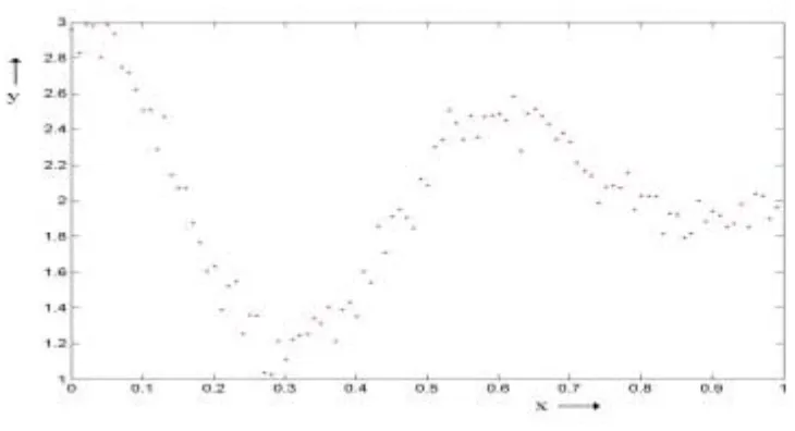
i (2.3)As an example, we choose example σ = 0.11 and n = 10, which means that there will be 10 Gaussian indicator function distributed over input space. Function (2.4) is chosen to generate a training set, which contains 100 samples and is shown in Figure 2.1.
Figure 2.1. Example dataset with 100 data points
With the input data and the kernel function (2.2) indicator matrix X is formed; it will have a size of [N x n] where N is the number of data points and n is the number indicator functions (in this example N=100 and n = 10).
= ) ( ) ( ) ( ) ( ) ( ) ( ) ( ) ( ) ( 2 1 2 2 2 2 1 1 1 2 1 1 N n N N n n x f x f x f x f x f x f x f x f x f L M O M M L L X , = N y y y M 2 1 y , = n b b b M 2 1
b (2.5)
The first elements of this matrix X calculated for the example training set are shown below.
=
O
M
M
M
M
M
L
L
L
L
L
00
.
0
03
.
0
26
.
0
82
.
0
93
.
0
00
.
0
02
.
0
22
.
0
76
.
0
96
.
0
00
.
0
02
.
0
19
.
0
71
.
0
98
.
0
00
.
0
01
.
0
16
.
0
66
.
0
00
.
1
00
.
0
01
.
0
14
.
0
61
.
0
00
.
1
X
(2.6)Vectors x and y are input data and the latter is assumed to be corrupted by normally distributed noise, ε. By using the matrices introduced as above the following relation holds:
e
Xb
Xb
y
=
+
ε
+
φ
=
+
(2.7)In this formula ε is the normally distributed noise on the samples and φis the approximation error, which depends on the choice of the indicator function. The total approximation error e, is the sum of εand φ. The minimization of the summed squared approximation error is given as:
)
||
||
2
1
||
||
2
1
(
min
Xb
−
y
22+
λ
b
22b (2.8)
2 2 =
∑
i xix (2.9)
The term
||
||
222
1
b
is the so-called regularisation term that minimises the parameters and λ is apositively valued regularisation parameter. Taking the derivative to b of formula (2.8) and equating this derivative to zero yields:
y
X
b
I
X
X
T+
)
=
T(
λ
(2.10)or
y
X
I
X
X
b
=
(
T+
λ
)
−1 T (2.11)In this equation I is the identity matrix. By solving this equation the vector b is calculated and will have the size of [n x 1]. The values of b for the example are given below.
[
]
T47
.
1
41
.
0
81
.
0
99
.
0
28
.
1
63
.
0
33
.
0
31
.
0
92
.
0
35
.
2
=
b
(2.12)With parameter vector b known, it is possible to give an estimate for a new sample xnew.
b
x
f
x
x
n)
(
n)
(
)
(
ˆ
1
new n
i
ew i i ew
b
f
y
=
∑
=
=
(2.13)
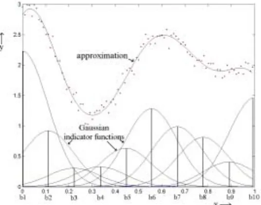
The parameter vector b contains the weights of the Gaussian indicator functions, which have been drawn as vertical bars in Figure 2.2. By summing the weighted evaluations of the indicator functions the approximation is constructed. The samples in the training set are depicted by the (red) dots. As one can see for this particular situation a good approximation is obtained.
2.2 Dual Least Squares function approximator
The Ordinary Leas Squares algorithm divides the input space into regions, as a result of the choice of the kernel functions. In the example of section 2.1 the input space (x∈
[ ]
0,1), was divided into ten different regions by the Gaussian indicator functions. The disadvantage with this approach is that every part of the input space is mapped into feature space even if there are not any data points present in that part. Hence, although no data may be given for a part of the input space, one does have to take that part of the input space into consideration. Putting the minimization problem of (2.8) in a dual form helps to circumvent this non-data-driven mapping from input to feature space. The minimization problem can be written as (De Kruif, 2004):)
2
1
2
1
min(
e
Te
+
λ
b
Tb
(2.14)with
Xb
y
e
=
−
(2.15)in which e is a column-vector containing the approximation error for all the samples. When e is minimized, ideally it consists of only the noise, which contaminated the training set. This means that and in this case e=ε from (2.7). From (2.14) a Langrangian can be constructed:
)
(
2
1
2
1
e
Xb
y
a
b
b
e
e
+
+
−
−
=
T T TL
λ
(2.16)The vector a consists of the Lagrangian multipliers and has the same dimension, N, as the number of samples. The minimisation problem (2.14) can be solved by equating the derivatives of the Langrangian with respect to b, e and a to zero. The solution of (2.16)
gives the expression:
y
a
I
XX
+
)
=
(
Tλ
(2.17)In section 2.1, the solution was given as:
y
X
b
I
X
X
T+
)
=
T(
λ
(2.18)These solutions are identical if the following holds.
a
X
b
=
T (2.19)The estimation of output for the new input values can be calculated as follows:
a
X
x
f
b
x
f
x
new new new Ty
ˆ
(
)
=
(
)
=
(
)
(2.20)in summation form, this can be written as:
i N
i
i new new
n
i i i
new
b
f
x
a
y
∑
∑
= =
=
=
1 1
)
(
),
(
)
(
)
(
ˆ
x
f
x
f
x
(2.21)Where f(xnew),f(xi) is the inner product of vector f(xnew) and f(xi) and in which vector f(xi)
The point to observe here is that calculation of the inner product does not require explicit calculation of f(xnew). Hence the prediction with the use of a is not depending on the number of
kernel functions but only on the number of samples N. Therefore, it is possible to use a large or even an infinite dimensional feature space for the approximation. When training with data sets that are relatively small and not homogenously spread over input space, the DLS algorithm will probably be more efficient than the OLS algorithm. However, the data contained by vector a in the DLS algorithm is abstract compared to that of vector b in the OLS algorithm and therefore it is more difficult to check whether the implemented DLS algorithm works properly.
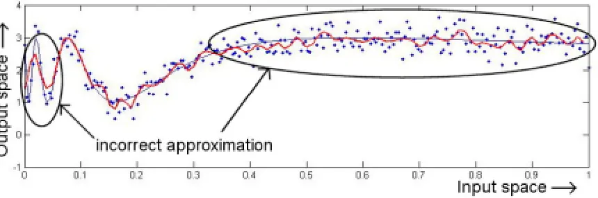
However dual and ordinary least squares function approximators are commonly used they are not able to approximate certain functions. This training set of these functions is corrupted by measurement noise and the function itself has large differences in its derivative values. In Figure 2.3 it the least squares algorithm is unable to approximate the function in areas, which it has, large absolute values for its derivative. Furthermore in the area where the derivative is small the algorithm starts to fit the measurement noise.
Figure 2.3. Least squares approximation
3 Existing Key Sample Machine algorithms
Key Sample Machines were developed to approximate functions in a more sophisticated way compared to ´Ordinary Least Squares´, ´Dual Least Squares´ or even ´Support Vector Machines´. The goal was to develop an algorithm that (De Kruif, 2004):
• Uses the summed squared approximation error as cost function
• Uses a sample-based approach in which the prediction parameters are trained by using the inner product between the samples
• Uses some of the samples for the prediction, but use all the samples for the training (data compression)
• Uses a subset selection scheme that fits the problem at hand to select the samples that are to be used for a proper prediction.
The KSM algorithm combines advantages of several function approximation algorithms and is therefore more accurate, less time consuming or less demanding on computer-resources.
3.1 Offline Key Sample Machine
The offline Key Sample Machine (KSM) makes an approximation of the target function based on all samples in the training set (De Kruif, 2004). The first step is to treat all samples as potential key samples. That means that for every sample i, there is a corresponding kernel function fi. The kernel
functions span the so-called feature space into which all samples are projected. So if the training set consists of N samples it results in a matrix with dimension [N x N] in which the projected sample information is contained. This matrix is called the potential indicator matrix Xpotential:
= ) ( ) ( ) ( ) ( ) ( ) ( ) ( ) ( ) ( 2 1 2 2 2 2 1 1 1 2 1 1 N N N N N N potential f f f f f f f f f x x x x x x x x x X L M O M M L L (3.1)
In this matrix each column represents a potential key sample. These potential key samples have to be assessed, so a selection can be made which potential key samples will become “real” key samples. The latter will be used in the approximation of the function. The “real” key samples n, will, the construct indicator matrix X [N x n]:
= ) ( ) ( ) ( ) ( ) ( ) ( ) ( ) ( ) ( 2 1 2 2 2 2 1 1 1 2 1 1 N n N N n n f f f f f f f f f x x x x x x x x x X L M O M M L L (3.2)
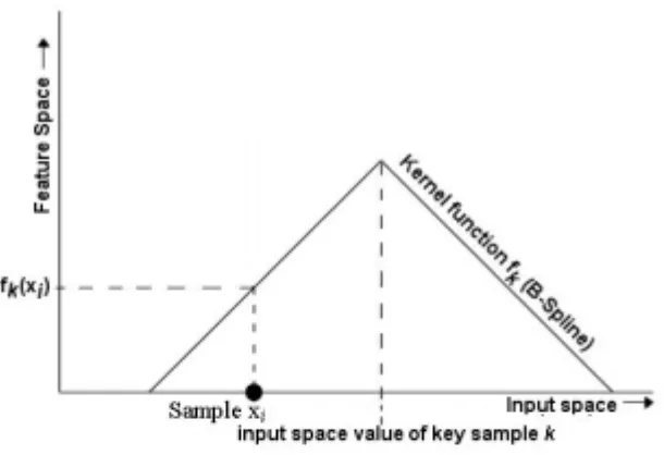
Figure 3.1. Projection of a sample into feature space by a B-spline kernel function
To approximate the target function, the kernel functions, which are characterized by the key samples, are given a weight. In Figure 3.2, four key samples are used for the approximation. This means that four kernel functions (in this particular case B-splines) are defined and each has a certain weight (w1…w4). By summing the kernel functions the output values of the target function are predicted.
Figure 3.2. Function approximated with four B-spline kernel functions
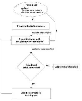
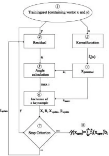
Figure 3.3. Simplified block diagram of the offline KSM algorithm
In Figure 3.3, a simple block diagram of the offline KSM algorithm is depicted. All steps of this algorithm will be treated in more detail below.
3.1.1 Training
Set
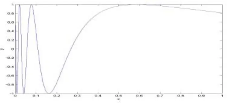
First a dataset with training samples is needed. This training set contains N samples, which are stored in the input and output vector (x and y). When evaluating the performance of an algorithm, it is important to choose a proper training set. By choosing a training set, which has a large difference in absolute value of its derivative, it is possible to test whether the approximator can handle different fluctuation speeds or not. Formula (3.3) can be used to create a training set with such characteristics.
ε
+
+
=
sin(
1
)
v
x
y
(3.3)Figure 3.4. Function with large differing derivative values
3.1.2 Create
potential indicators
In the process of creating potential indicators two steps can be distinguished. First the samples have to be projected into feature space. Second the projected samples are used for creating potential indicators.
3.1.2.1 Kernel function
The input vector x is projected into feature space by selected kernel functions. Any function can be selected as kernel function. However, by selecting kernel functions, the total set of possible functions that can be approximated, is determined. It is important that the function that has to be approximated is an element of the set of possibilities. In other words, the kernel functions have to be chosen in a way such that the target function is linear in feature space. In most cases, the structure of the target function is unknown; therefore kernel functions giving a large set of possibilities are preferred. Infinite splines or B-splines can approximate any function that has a certain maximum value for its derivative. The formula for first order B-splines is given as a convolution below:
) ( * ) ( )
( 0 0
1
c c
c f x x f x x
x x
f − = − − (3.4)
with
−
≤
−
<
=
elsewhere
x
x
if
f
c0
5
.
0
5
.
0
1
0
(3.5)
The first order B-spline function has a triangular shape with its centre at xc. In the same way as in
the example in section 2, altering the height of the splines can approximate the target function. In the OLS algorithm the whole input space is projected into feature space. In the DLS algorithm, that part of the input space that contains data points is projected. In KSM, this dual projection is also applied. Each sample in the training set represents a potential indicator function, which is in this case a B-spline. The centres of these splines correspond to the x-values of the samples in the training set. Therefore, there are no indicator functions in those parts of the input space that do not contain any samples.
The notation of a dual indicator function is given below.
) , ( ) ( ~
i i f
The dual indicator function
f
~
will project all samples x, from input space to that part of feature space, which is spanned by sample xi. In case of B-spline indicator functions, xi is the same as xc informula (3.4). In Figure 3.5 a data set with four training samples is drawn. Each sample is considered as a potential key sample. Therefore all samples generate a potential B-spline indicator function, indicated with A, B, C and D in this figure. Each sample is projected on each B-spline. For example, the value A1 (on the y-axis) stands for the y-value of the projection of sample 1 on B-spline A.
Figure 3.5. Training set with four samples and four potential B-spline indicator functions
3.1.2.2 Creating potential indicator matrix (Xpotential)
The projections from input to feature space are stored in a matrix called Xpotential. In this matrix
every column represents a key sample, which potentially can be used for the approximation.
=
) 2 1 2 2 2 2 1 1 1 2 1 1(
~
)
(
~
)
(
~
)
(
~
)
(
~
)
(
~
(
)
~
)
(
~
)
(
~
N n N N n n potentialf
f
f
f
f
f
f
f
f
x
x
x
x
x
x
x
x
x
X
L
M
O
M
M
L
L
(3.7)3.1.3 Select indicator with maximum error reduction
Before adding one of the potential key samples to the real set of key samples, it is necessary to know which potential key sample will reduce the approximation error the most. This selection procedure consists of two steps, which are treated in detail in this paragraph.
3.1.3.1 Determining the residual
=
4
4
4
4
3
3
3
3
2
2
2
2
1
1
1
1
D
C
B
A
D
C
B
A
D
C
B
A
D
C
B
A
potential
X
(3.8)Determining which potential key sample has to become a real key sample is done as follows. The residual e, is the difference between the function output values of the trainings set (y) and the predictions (Xb) of the function output values:
Xb
y
e
=
−
(3.9)The matrix X is called the indicator matrix and contains the previously selected key samples. Initially it contains only the value one and has the size of [N x 1]. Initially adding key samples to the matrix X results in a more accurate approximation and therefore a smaller residual. However, when all samples are included as key samples, noise is being fitted into the approximation. Therefore there is an optimum in the number of samples that are used as key samples. In practice there always is a demand for a certain level of accuracy of the approximation. The optimal solution will be to include the minimal amount of key samples in the matrix X that suffices to approximate the target function with the demanded accuracy. This can be done by recursively including a potential key sample that gives the largest reduction of the residual.
3.1.3.2 Calculating the angle between indicator vectors and the residual
The column vectors (ai), in matrix Xpotential represent the potential key samples in feature space. By
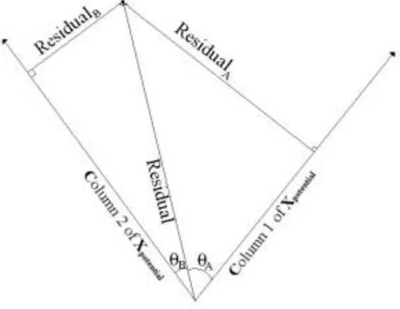
calculating the angle between these potential key samples and the vector e, it is possible to determine which potential key sample will reduce the residual most when added to X. This is shown in Figure 3.6.
Figure 3.6. Angle between key samples and residual
In this figure two key samples and the current residual are drawn. ResidualA and ResidualB are the
residual. Ideally the angle is zero and the residual will be entirely eliminated but this will in general not be the case. The angle between the residual and the key samples can be calculated with formula (3.10).
)
(
)
(
)
cos(
2 2
e
e
a
a
a
e
T i T i
i T
i
err
=
θ
=
(3.10)Inwhich erri is the normalised change in error due to the inclusion of potential indicator i. The
vector ai is the i-th column vector in Xpotential, corresponding to the indicator defined by the i-th key
sample. The key sample that results in the largest decrease in error should be selected for inclusion.
3.1.4 Add key sample to existing set
For a stable and relative fast inclusion of a key sample it is necessary to apply QR-decomposition onto matrix X. First this decomposition will be explained and second the actual inclusion will be treated.
3.1.4.1 QR-decompositon
The selected potential indicator (amax i) will be added to indicator matrix X. With this ´updated´
matrix the vector b, which is used for the approximation of the function, can be calculated in the same way as in the OLS algorithm.
y
X
b
X
X
T)
=
T(
(3.11)Calculating vector b with this formula is demanding on computer resources, because the inverse of (XTX) has to be calculated. By applying QR-decomposition on the indicator matrix X, vector b can be calculated without explicitly determining this inverse and therefore extensive calculations are evaded. If X is of full column rank, QR-decomposition implies that that:
[
]
=
⊥0
R
Q
Q
X
X (3.12)In which QX forms an orthogonal base for the column vector space of X and Q⊥ an orthogonal base
for the null space of X. Matrix R is an upper triangular matrix in which the information about the relation between X and Q is stored. For example, suppose the training set contains three samples from which the first two samples are key samples. In Figure 3.7 this situation is sketched with first order B-splines as kernel function.
The indicator matrix X will be in the form:
=
=
5 . 0 0
1 5 . 0
5 . 0 1
3 3
2 2
1 1
B A
B A
B A
X (3.13)
The feature space, which is spanned by the column vectors of X is two dimensional. This 2-dimensional feature space is spanned within 3-2-dimensional row space in which the axes are respectively ~fi(x1),~fi(x2), f~i(x3) with i∈(1,2). The vector space of QX forms an orthonormal
base for the feature space and Q⊥ forms the orthonormal base for the null space of X. This is drawn
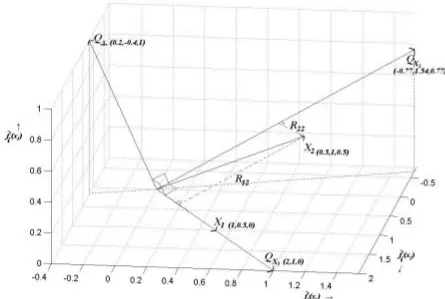
in Figure 3.8. The column vectors of Q have been drawn in the correct direction but the lengths are not normalized to avoid an indistinct figure.
Figure 3.8. Column space of X (expression (3.13)) and column space of accompanying Q
The vector QX1 has per definition the same orientation as vector X1. Vector QX2 is perpendicular to
QX1 but will be in the same plane as X1 and X2. This plane represents the feature space and is
perpendicular to the null space Q⊥. The matrix R is an upper-triangular matrix, from which element (1,1) is the inner product between QX1 and X1. Because all QX column vectors are orthonormal the
other elements in the first column of R will be zero. The second column of R will only have non-zero values on the first two elements. In Figure 3.8 the vector X2 is projected on QX1 and QX2. The
projection values are stored in respectively R12 and R22. The other elements in this column will be
zero because of the fact that the column space of Q is orthonormal. Via this reasoning it can be seen that R will be an upper-triangular matrix by construction.
− − − − − = 8018 . 0 5976 . 0 0 5345 . 0 7171 . 0 4472 . 0 2673 . 0 3568 . 0 8944 . 0 Q , − − − = 0 0 8367 . 0 0 8944 . 0 1180 . 1
R (3.14)
The first column vector of Q has the same direction as the first column vector of X. Element (1,1) of R, is the projection of the first column vector of X onto the first column vector of Q. The second column vector of Q is orthonormal to the first column vector of Q. Therefore Element (2,1) of R, which is the projection of the first column vector of X onto the second column vector of Q, is zero. The rank of X is two for this example, however the two column vectors are defined in a three-dimensional space. So the orthonormal basis of Q also spans a three dimensional space. The column vectors of X can maximally span a two-dimensional space, so that means that one dimension spanned by the column vectors of Q is the so-called null space. This space cannot be “reached” by any combination of the two column vectors of X. In Figure 3.8, this null space is spanned by Q⊥. The residual vector, which is calculated in paragraph 3.1.3.1, is for this example
defined in the same three-dimensional space as X. When this residual vector has a non-zero element within the null space it is impossible to reduce this part of the error by means of the existing key samples. If this error is larger than the accepted error, a new key sample has to be added. By adding this key sample the rank of X will become three and therefore there is no null space. The residual vector can be reduced until it contains only the measurement noise.
In the example above the training set consists of three samples. In practice training sets will consist of about 100-100.000 samples. If the training set consists of N samples of which there are n key samples selected the indicator matrix X will be of the size [N x n]. Because of the angle calculation with which key samples are selected, key samples will never be identical and therefore never generate the same column vector. This means that the rank of X will be always equal to n. The null space Q⊥will be equal to N-n, which is also true for the example. If the indicator matrix has the
form: = Nn N N n n X X X X X X X X X L M O M M L L 2 1 2 22 21 1 12 11
X (3.15)
Q will have the form:
[
]
4 4 4 3 4 4 4 2 1 L M O M L L 4 4 4 4 3 4 4 4 4 2 1 L M O M M L L ⊥ = = + + + ⊥ Q NN n N N n N n Q Nn N N n n X Q Q Q Q Q Q Q Q Q Q Q Q Q Q Q ) 1 ( 2 ) 1 ( 2 1 ) 1 ( 1 2 1 2 22 21 1 12 11 X Q QQ (3.16)
and R will be:
= = nn n n nn n n n n R R R R R R R R R R R R R R R 0 0 0 0 0
0 22 2
1 12 11 2 1 2 22 21 1 12 11 M O L L L M O M M L L
X will always be of full column rank, because identical potential key samples will not be selected to be included in X. The solution of the least squares problem of minimizing
||
y
−
Xb
||
22 will beuniquely determined by the QR equation
X
z
y
Q
Rb
=
TX≡
(3.18)The goal is to calculate b without using formula (3.11). From the formula above it can be seen that
b can be calculated by:
b=zx/R (3.19)
Augmenting X with y and then performing QR-decomposition on this augmented matrix Xa makes
it possible to calculate zx. The QR-decomposition of Xa is shown below:
Xa=QaRa (3.20)
[
]
=
2 2 0 || ||
||
|| r
z R
r r Q y
X X (3.21)
The R matrix of the QR-decomposition can be found by means of Cholesky decomposition, without the necessity to calculate the corresponding Q. When X has a full column rank, then the Cholesky decomposition of XTX exists:
chol T chol T
R R X
X =: (3.22)
Substitution of the QR-decomposition for X in XTX yields:
R R QR Q R X
XT = T T = T (3.23)
From which it follows that the Cholesky decomposition of XTX equals the R of the QR-decomposition of X, because both are upper-triangular.
chol T
)
(
X
X
R
=
(3.24)The advantage is that the matrix Q is not needed in any of these calculations and can be omitted to save memory space.
So, in order to solve the OLS problem, we first create an augmented indicator matrix Xa. By means
of Cholesky decomposition the Ra and the corresponding zx are found. With these, the parameter
vector b can be calculated.
3.1.4.2 Inclusion of a key sample in QR-decomposition
When a potential key sample is selected as candidate to become a ´real´ key sample, the indicator matrix X has to be extended with one column. As seen in section 3.1.1 the Cholesky decomposition of
(
X
TaX
a)
results in Ra. To circumvent calculating the Cholesky decomposition each time a keysample is added to X it is necessary to know in what way Ra changes. Before the update relation
(3.24) holds, so that:
a T a a T
a
X
R
R
when written out, the result is:
[
] [
]
=
ρ
ρ
0
0
r
R
r
R
y
X
y
X
T T (3.26) + = 2ρ
r r R r r R R R y y X y y X X X T T T T T T T T (3.27)This gives the following equalities:
RTR=XTX (3.28a)
RTr=XTy (3.28b)
yTy=rTr+ρ2 (3.28c)
After the update Xa will have the form:
[
X
x
y
]
X
a=
(3.29)In which X is the existing indicator matrix, x is the key sample to be added and y is the vector that contains all the output values of the training set. Then Ra will be:
=
τ
ρ
γ
0
0
0
r
g
R
R
a (3.30)After the update the following relation still has to hold:
a T a a T
a
X
R
R
X
=
(3.31)If (3.29) and (3.30) are filled in (3.31) the result is:
+
+
+
+
+
=
2 2 2τ
ρ
ρ
γ
ρ
γ
γ
r
r
g
r
R
r
r
g
g
g
R
g
r
R
g
R
R
R
y
y
x
y
X
y
y
x
x
x
X
x
y
X
x
X
X
X
T T T T T T T T T T T T T T T T T T (3.32)In combination with (3.28) the following relations can be derived. These relations are used to update the matrix Ra:
R
R
=
(3.33a)γ
2=
x
Tx
−
g
Tg
(3.33d)x
X
R
g
=
−T T (3.33b)=
1
(
x
Ty
−
g
Tr
)
γ
ρ
(3.33e)r
r
=
(3.33.c)τ
2=
y
Ty
−
r
Tr
−
ρ
2 (3.33f)3.1.5 Stop
Criterion
Including key samples to X will make the prediction more accurate. However, including all potential key samples in X is too demanding on computer resources and there would not be any data compression. The first key samples, which are included to X will largely improve the accuracy of the prediction, but every key sample included will result in a smaller improvement than its predecessor. Especially if the training data set is contaminated with noise, it could be that adding extra key samples will result in fitting noise into the approximation. Therefore, it is necessary to implement a criterion, that states when to stop the inclusion of key samples. Define the extra sum of squares S2 as the difference between the summed squared approximation errors of all samples before and after the inclusion of the potential key sample. If the output values of the trainings set are contaminated with additive Gaussian noise with a variance of σ2, then:
2 2
σ
S
~
2 1χ
⇔
ai=0 (3.34)Here
χ
12denotes a chi-square distribution with one degree of freedom. A potential key sample aiwhich contains no information, is denoted as “ai=0”. If ai is zero, than the probability that a certain
error reduction is found is calculated as:
ζ
σ
≥
ζ|
=
0
)
<
(
22
a
z
S
P
(3.35)In this equation ζ denotes the probability that a realisation of zζ or larger is found. ζ is called the
significance level and the corresponding value of zζ follows from the
χ
12distribution. The factor2 2
σ
S
is used as a measure for the error reduction of the approximation. So what is being calculated
is the chance of having a certain error reduction given that the vector a is zero (contains no information). If this chance is very small it means that a is probably unequal to zero. If it would be equal to zero it would be very improbable that the given error reduction would occur. In Figure 3.9 this is explained graphically.
In the figure above the horizontal-axis represents the value of 2
2
σ
S
. The chance of having this error
reduction with given that a is zero, is equal to ζ (shown as the grey surface). This figure shows clearly that the larger the error reduction, the chances of vector a containing no information becomes smaller. If the chance of having a certain error reduction with a=0 is very small then this new parameter is probably unequal to zero and should therefore be included as a key sample.
3.1.6 Approximate the function
When the function approximator has extracted the information from the training set, it has “learned” the target function. The approximator is able to give an output value of the function for any given input, which lies within the input space of the training set. The function output value is calculated as:
∑
=
=
ni
i new i
new
f
b
y
1
)
(
~
)
(
ˆ
x
x
(3.36)
Here b is calculated as in (2.11) and f~iis the indicator function described by formula (3.6). It can be seen that the approximated output value is calculated summing the multiplications of each indicator function with its corresponding weight.
In Figure 3.10 a detailed block diagram of the offline KSM algorithm is shown. Here are all previously treated steps shown in relation to each other.
3.1.7 Matlab
Results
The offline algorithm described in this section has been implemented in Matlab. The Matlab code is included in Appendix B. The offline KSM is tested by approximating function (3.3). First a data set with 250 samples is generated and these are presented to the algorithm. The graphical output of the algorithm is shown in Figure 3.11. This approximation uses 23 key samples. Compared with the 250 samples in the original dataset it means there is a reduction of 90 % in the number of used samples.
In Figure 3.11 the dots are the samples in the training set, which are corrupted by Gaussian noise in their output values. The line represents the approximation made by the offline KSM. In the area where the derivative is relative small there is no or very little fitting of noise into the approximation. The area where the function has large derivative values the offline key sample machine is in contrast to the least squares approximators, capable of approximating the function rather well.
3.2 Online Key Sample Machine
In section 3.1 it was shown that the offline KSM makes an approximation based on the information contained by all the samples in the training set. All samples are at the same time available to the algorithm. By selecting samples that contain most information as key samples, it is possible to approximate the function with a minimum of kernel functions. However, in practice it cannot always be guaranteed that all samples will be available beforehand. When the function approximation is done while the system that has to be controlled, is in operating mode, samples will become available one at a time. Storing these samples to construct a training set, which contains enough samples that are well distributed over input space, will take time. This especially will be the case if the system only works in certain areas of the input space for longer periods of time. During the period that the training set is being constructed the feed-forward controller cannot improve the performance of the system. This is a major drawback of the offline KSM algorithm. Therefore an online key sample machine was developed.
The online or Recursive Key Sample Machine (RKSM) approximates functions recursively. This means that RKSM is presented with one sample at a time and updates the approximation with the information contained by this sample. Therefore it is possible to make an approximation without having to wait for a training set with enough well distributed samples. The feed-forward controller can improve the performance of the controlled system from the moment it receives information about the system contained by incoming samples. Because of this continuous updating, RKSM is able to approximate even when the target function is somewhat dynamic because of changing system parameters (e.g. temperature). The disadvantage of recursive approximation is that when only few samples have been received, it is impossible to determine the amount of relative information contained by these samples. Therefore the assignment of key samples is especially in the beginning, non optimal. This however is later on corrected by evaluation key samples and removing those, which contain not enough information.
The RKSM algorithm can perform three approximation-updating actions. These are:
- Fine tuning the current approximation based on an incoming sample - Extending the set of key samples with an incoming sample
- Omitting a key sample which contains not enough information
The updating actions will be treated here. An incoming sample is considered lying inside the uncertainty boundaries of the existing approximation. These boundaries are caused by measurement noise on the samples and consequently causing uncertainty in the approximation.
Figure 3.12. Incoming sample is used to fine tune key samples
When an incoming sample is lying outside the uncertainty boundaries fine-tuning the existing key samples does not suffice. A structural change has to be made by extending the set of key samples with the incoming sample. This is drawn in Figure 3.13.
Figure 3.13. Inclusion of a key sample
Because there is no knowledge about future samples it is impossible to determine the amount of information an incoming sample contains. In coming samples can only be compared with previous samples. Therefore the first samples have a large probability of becoming key samples. It is possible that a sample that was included as a key sample, contained a relative large amount of information in the early stages of the approximation, but has a relative small contribution when more samples have been presented to the RKSM. The RKSM will evaluate the relative amount of information of each key sample and if the contribution of a certain key sample is to small, it will be omitted. If the approximation after omission lies within the uncertainty boundaries the key sample can be omitted. This is graphically explained in Figure 3.14.
Figure 3.14. Omission of a key sample
Figure 3.15. Block diagram of RKSM algorithm
3.2.1 Incoming
sample
The input for the RKSM consists of one sample at a time. The number of samples in the training set is not limited to certain values. RKSM will include information from incoming samples continuously, unless the user chooses to limit this “learning” period. As with KSM, for a good approximation it is important to have sufficient well-distributed samples.
3.2.2 Kernel function
The kernel functions, which have been treated in section 3.1, have the same purpose in RKSM as they have in KSM.
3.2.3 Fine-tuning
In the KSM algorithm all samples N, are used to create the indicator matrix Xpotential [N x N]. The
column vectors that carry the most information about the target function are selected and become key samples n, with which indicator matrix X [N x n] is constructed. It is impossible to implement this procedure in RKSM because of:
- The unlimited amount of samples in the training set and the corresponding infinitely large indicator matrix Xpotential and X.
- Only samples that already have been presented to the algorithm are known, there is no informationabout future samples and therefore these samples cannot be used to construct
Xpotential.
To circumvent this problem the following is done:
With the samples in the training set, two sets are constructed. Reduced set: This set contains only the n key samples
Full set: This set contains all the training data
Matrix Xks is the indicator matrix for the reduced set and is defined as in formula (3.37).
=
) 2 1 2 2 2 2 1 1 1 2 1 1(
~
)
(
~
)
(
~
)
(
~
)
(
~
)
(
~
(
)
~
)
(
~
)
(
~
n n n n n n ksf
f
f
f
f
f
f
f
f
x
x
x
x
x
x
x
x
x
X
L
M
O
M
M
L
L
(3.37)The matrix Xks has a dimension of [n x n] and contains the kernel function values for all key
samples. Matrix X, which is also used in KSMis defined as:
In order to let the key samples represent the complete data set, a weight is introduced so that the normal and weighted normal equation become identical. This matrix Xks is related to indicator
matrix X [N x n] in the following way:
ks T
ks T
X
V
X
X
X
=
−1 (3.39)The non-weighted (3.11) and weighted normal equations are given in formula (3.40) and (3.41).
y
X
Xb
X
T=
T (3.40)ks T
ks ks
T
ks
V
X
b
X
V
y
X
−1=
−1 (3.41)Matrix V-1 [n x n] is the covariance matrix, which is used in weighting the key samples. The weight indicates how much information each key sample contains related to the other key samples. The non-weighted and weighted normal equations have to be identical. If the left-hand sides of the equations are made equal, it follows that:
1 1
1 − − −
−
⇒
=
=
T T ksks ks
T ks T
X
X
X
X
V
b
X
V
X
Xb
X
(3.42)The same for the right-hand side:
X
Ty
=
X
TksV
−1y
ks (3.43a)y
X
VX
y
ks=
ks−T T (3.43b)
=
X
ks(
X
TX
)
−1X
−ksTX
−ksTX
Ty
(3.43c)
=
X
ks(
X
TX
)
−1X
Ty
(3.43d)This means that the output of the key samples yks is equal to the prediction of the full data estimator
at the key samples. The prediction of the reduced approximator is given as:
b
X
x
y
ks(
ks)
=
ks (3.44)Substituting (3.41) for b into this equation gives:
ks T
ks ks T
ks ks ks
ks
x
X
X
V
X
X
V
y
y
(
)
=
(
−1)
−1 −1 (3.45a)
=
X
ks(
X
TX
)
−1X
TksX
ks−TX
TXX
−ks1y
ks=
y
ks (3.45b)From this it can be concluded that the predictions of the full data approximator (3.43d) and the reduced approximator (3.45b) are equal.
For computing convenience X and Xks are QR-decomposed.
QR
X
=
(3.46)ks ks ks
Q
R
X
=
(3.47)Formula (3.39) can be written as:
ks T ks T
ks ks T
R
R
V
R
R
R
R
=
−1 (3.48)T ks T ks T T ks T
ks
R
R
RR
R
R
V
−1=
− − (3.49)The algorithm uses and stores only the matrices R, Rks and V-1. If a sample is presented to the
RKSM algorithm the input space information is projected into feature space, by the kernel functions. This information is used to fine-tune the existing key samples. As the number of key samples does not alter, the matrices X and Rks remain unchanged. The augmented indicator matrix
is extended by a row due to the new training sample.
[
]
=
⇒
=
y
a af
y
X
X
y
X
X
(3.50)In which y is the output value of the incoming sample and f is a vector that contains the output of the kernel functions for the x-value of the incoming sample. Instead of using Xa the algorithm uses
the matrix Ra from the QR-decomposition of Xa. Matrix Rais stored in its augmented form as it is
done in KSM. The information of the incoming sample will change the augmented R matrix in the following way:
[
]
=
⇒
=
y
a af
z
R
R
z
R
R
X X (3.51)By means of a Givens rotation, this matrix is reduced in the following form:
= ⇒ =
ς
0 z R R f z RRa X a X
y (3.52)
In which
R
is upper-triangular and ζ2 is the change in summed squared error due to the new sample. The Givens rotation algorithm calculates an angle by which the orthonormal basis spanned by Q is rotated. Matrix R contains the projections of X on this basis of Q. This rotation is done in such a way that matrix R becomes upper-triangular again. The Givens rotation is explained in detail in appendix A.The weight matrix V-1 relates the matrix R and Rks as shown in (3.48). The weights indicate the
number of samples each key sample represents. Therefore the weights have to be updated when the key samples have been fine-tuned. The updated matrix V-1can of course be calculated with (3.48) but it demands less computing resources to update the weight matrix as follows:
T T ks ks
R
f
R
u
=
−1 − (3.53a)u
u
V
V
−1=
−1+
T (3.53b)In (3.53)
R
ksis the fine-tuned matrix Rks and 1 −V
is the updated weight matrix.3.2.4 Inclusion selection criterion
samples. In that case the sample will be included as will be described in paragraph 3.2.5. When the summed squared error is relatively small the RKSM algorithm will proceed with selecting potentially omitted key samples, which is treated in 3.2.6.
3.2.5 Inclusion of a key sample
A sample that has to be added to the set of key samples will affect matrices R, Rks and V -1
. The weight matrix V-1will be extended with one row and one column, as done in (3.54).
= − − 1 1 1 0 0 V V (3.54)
Here
V
−1 is the updated weight matrix. Because the samples that were presented previously to the RKSM were not stored, it is impossible to determine the covariance between these samples and the current incoming sample. Therefore an assumption is made that the incoming sample is uncorrelated with the previous