Entropy Reduction for the Correlation-Enhanced Power Analysis Collision Attack

Entropy Reduction for the Correlation-Enhanced

Power Analysis Collision Attack

Andreas Wiemers, Dominik Klein[0000−0001−8174−7445] Bundesamt f¨ur Sicherheit in der Informationstechnik (BSI)

{firstname.lastname}@bsi.bund.de

Abstract. Side Channel Attacks are an important attack vector on se-cure AES implementations. TheCorrelation-Enhanced Power Analysis Collision Attackby Moradi et al. [MME10] is a powerful collision attack that exploits leakage caused by collisions in between S-Box computations of AES. The attack yields observations from which the AES key can be inferred. Due to noise, an insufficient number of collisions, or errors in the measurement setup, the attack does not find the correct AES key uniquely in practice, and it is unclear how to determine the key in such a scenario. Based on a theoretical analysis on how to quantify the remain-ing entropy, we derive a practical search algorithm. Both our theoretical analysis and practical experiments show that even in a setting with high noise or few available traces we can either successfully recover the full AES key or reduce its entropy significantly.

1

Introduction

Kocher’s [Koc96] groundbreaking paper on side channel attacks has led both science and industry to focus on attacking and hardening their implementa-tions [AARR03]. Due to its popularity and de-facto standard w.r.t. symmetric cryptographic algorithms, AES [BCO04,GMO01,KJJ99,Nat01,QS01] is of par-ticular interest. Despite its theoretical cryptographic strength, a secure AES implementation that does not leak information about processed data remains to be a challenge. A popular counter-measure to minimize leakage about the AES key is masking. Different masking schemes exist, but the general idea of mask-ing is that whenever secret data is about to enter critical stages of operation, some reversible operation that makes the data appear to be random is applied. Any cryptanalysis of intermediate data of the processing step is thus worth-less. After leaving the critical stage of operation, the operation is reversed and the processed result can be used. Appropriate masking schemes can successfully prevent several attacks.

collisions are of interest. This kind of attack method was originally applied to DES [LMV04,SWP03], but later applied to AES [Bog08,SLFP04] as well.

A very powerful kind of collision attack against AES was applied in [MME10], and later improved in [CFG+_{11], and reconsidered in [MS16]. The attack works} by feeding data into a device in order to create collisions. A major important observation by [MME10] is that since the S-Box in AES is mathematically the same for every key byte (as opposed to i.e. DES), in most implementations the S-Box is also the same for every key byte. For example in a software implementation there is likely only one S-Box procedure that is called for every key byte, and in the case of a hardware implementation there is a single S-Box circuit that is used to process every key byte. This implies that for two same processed values, the resulting power consumption should be the same as well. Their idea is to create collisions such that this leakage between S-Box computations of different key byte positions is exploitable. This makes the attack very powerful — it is shown in in [MME10] that a device with S-Boxes that are masked using the Canright S-Box implementation [Can05,CB08] can be broken with a reasonable amount of available traces. It is important to note here that in general the leakage of the device attacked in [MME10] was minimal, and in particular a typical state-of-the-art template attack [CRR03] was close to impossible to execute. In particular the amount of trace data needed to mount a successful attack was magnitudes lower for the correlation attack than for a template attack.

The attack gives some information about the correct AES key. However, the attack might not find the correct AES key uniquely in practice. There are several reasons for this: Noise, an insufficient number of collisions, errors in the mea-surement setup, or simply the device itself, i.e. the design and implementation of the cryptographic co-processor for a hardware implementation, or the proces-sor design and execution flow in a software implementation. Moreover, it is not clear a priori how to find a set of key candidates that fit to the observations of the attack. A naive approach, i.e. enumerating all possible key candidates is computationally infeasible due to the large search space.

It is also unclear how to assess the leakage of the device; in particular it leaves open the question how many measurements (traces) are required to successfully mount the attack. Obviously, if the key uniquely identified for a certain amount of traces, this gives an upper bound. However what if less measurements are available?

In this paper we provide an algorithm to recover the AES key in the above scenario. The theoretical motivation of the algorithm is the basis for our analysis on how to quantify the remaining entropy, which can be used to assess the leakage of a device. Both our theoretical analysis and practical experiments show that even in a fuzzy setting with high noise or few available traces, we can either successfully recover the full AES key or reduce its entropy significantly.

i.e. its impact on the entropy of a vulnerable system w.r.t. its leakage, and give upper and lower bounds of the remaining entropy. Our theoretical findings are verified by providing experimental data in Section 6. The algorithm presented here can be seen as a particular form of a key-search algorithm. In Section 7 we show how our algorithm relates to known existing key search algorithms, and to the generalization of [MME10] described in [MS16]. Finally, we conclude our presentation in Section 8.

2

Correlation-Enhanced Power Analysis Collision Attack

Let K1, . . . , K16 be the correct key which is used in the first round of an AES encryption. We denote by small letters k1, . . . , k16 candidates for the key. We briefly recall the Correlation-Enhanced Power Analysis Collision Attack as de-scribed in [MME10].

During the measurement phase we recordNpower consumption traces of the first round of an AES-128 encryption1_{. These traces consists of 16 single S-Box} computations. The measurement of each single S-Box computation is given as a vector of T numbers. We denote by bi,w,t this power consumption trace of a

single S-Box computation iof a known plaintext pw,i, 1≤i≤16, 1≤w≤N,

1 ≤ t ≤ T. As a first step we compute the average value Mi,β,t over all w

with β =pw,i. Secondly, for any i, j and t we derive the empirical correlation

coefficient Ci,j,α,t betweenMi,β,t and Mi,β⊕α,t for any byte value α, where we

treat β as a random variable uniformly distributed on all 256 byte values. At last, we set ci,j(α) for the maximum of all Ci,j,α,t, where t runs over all time

points.

The idea of this approach is as follows: If the measurementbi,w,t is slightly

dependent on the input byte pw,i⊕Ki of the S-Box computationi, the average

Mi,β,t depends onβ⊕Ki even more significantly. Now the input bytesβ⊕Ki

of S-Boxiandβ⊕Kj⊕αof S-Boxj are the same for the choiceα=Ki⊕Kj.

Therefore, we can hope that the correlationCi,j,α,thas — at least for somet—

a significantly higher value for the correct choiceKi⊕Kj ofα.

3

Recovering the AES Key

In this section we formulate our algorithm for computing candidates for the full AES key. We assume that we have given 120·256 values in the form

ci,j(α)

for 1≤i < j≤16, whereαruns over all byte values. If for each i, j the value ci,j(Ki⊕Kj) is always the highest among all ci,j(α), then it is easy to derive

the full key. Here we are interested in the situation, where for eachi, j, the value

1

ci,j(Ki⊕Kj) has only a tendency of being large compared to otherci,j(α) with

α 6= Ki⊕Kj. The idea of our approach is to consider the ad-hoc evaluation

function

B=X

i<j

ci,j(ki⊕kj)

for any key candidate (k1,· · · , k16) and choose the key candidate with the highest value inB. Since this is not feasible in a straightforward manner, we instead try to computeB via partial sums. To this end, we fix an integerW, resp. integers g2,· · ·, g16.

Algorithm 1Recovering the AES Key 1: Setk1= 0,S1={k1}andB1= 0.

2: fors= 1, . . . ,15do

3: foreach key candidatek1, . . . , ksinSs do

4: foreach value of the next key bytesks+1do

5: compute the evaluation function

Bs+1=Bs((k1, . . . , ks)) + X

1≤i≤s

ci,s+1(ki⊕ks+1)

6: end for 7: end for

8: select subset of candidatesk1, . . . , ks, ks+1w.r.t. some criteria and store inSs+1:

9: Variant I: SelectW candidatesk1, . . . , ks, ks+1 with largestBs+1

10: Variant II: Select allk1, . . . , ks, ks+1withBs+1≥gs+1

11: end for 12: return

Remarks and Observations We note some properties of Algorithm 1: Since Bs and B only depend on ⊕-sums of key bytes, we can choose one key byte

as a fixed value. Here, we setk1 = 0. The success probability of both variants of our algorithm for finding the correct key depends on the input parameters W, resp. g2,· · · , g16. Obviously, if we choosegs=Bs((Ki⊕Kj)), Variant II of

Algorithm 1 is guaranteed to output the correct key. However, in this case Ss

might become too large to store in practice. The parameterW can be treated as a measure of the workload (i.e. the number of computational steps) of Variant I of Algorithm 1. Both variants of the algorithm assume a fixed order of key byte positions. The result of the algorithm depends on that assumed order of the key bytes. One can repeat the algorithm with different orders, though. Ass grows, the order becomes less important. We investigate the effect of the order on the success of the algorithm in Section 6. The choice of the order could take into account the actual distribution of the valuesci,j(α). Thosei, jwith significantly

high values in ci,j(α) could be considered first. In a practical setting, visual

general however, we are more interested in the situation where ci,j(Ki⊕Kj)

is not automatically the highest value among the ci,j(α), but is only larger on

average over alli, j.

4

Theoretical Justification

In this section, we give a justification of the evaluation function B. To this end, we treat ci,j(α) for any i, j, α as a realization of a normally distributed

random variable. Note that technically, this assumption is not correct. First, correlation values are bound in [−1,1] and thus cannot be normally distributed. Second, we do not consider correlation values directly, but instead ci,j(α) is a

maximum of Ci,j,α,t over several time points t. We can easily force ci,j(α) to

be normally distributed by fixing one single time-point, and apply Fisher’s z transformation on the correlation values. In practice however, we can see that the correlationsCi,j,α,t for wrongα(cf. Figures 3a, 3b) lie within [−0.25,0.25].

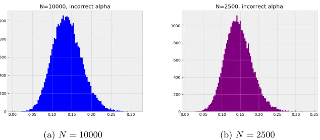
Fisher’s z transformation is almost identical for values in that interval, so that we do not consider this transformation in our case. In addition we observe (cf. Figures 5a, 5b) that the distribution ofci,j(α) is not perfectly symmetrical, but

minimally skewed. This can theoretically be justified by the fact that ci,j(α) is

a maximum of Ci,j,α,t over several time pointst. All in all, the deviation of the

distribution ci,j(α) from a normally distributed random variable is very small

and is thus neglected in the following.

We assume the easiest scenario: For anyi, j, αwithα6=Ki⊕Kj the means

and the standard deviations are equal and are denoted by a, resp. σ. Further-more, for the correct α=Ki⊕Kj the means are equal and are denoted by b

and in addition, the standard deviations are equal toσ. For any key candidate k= (k1,· · · , k16) we can check whether for all key candidates ˜k

ci,j(˜ki⊕˜kj)≈a, if ˜ki⊕˜kj =ki⊕kj

ci,j(˜ki⊕˜kj)≈b, if ˜ki⊕k˜j6=ki⊕kj

As a likelihood measure for any key candidate we seek a function in the single probability density functions as

1

√

2πσexp(−

(ci,j(˜ki⊕k˜j)−a)2

2σ2 ), resp. 1

√

2πσexp(−

(ci,j(˜ki⊕k˜j)−b)2

2σ2 )

density functions. Taking logarithms we get

X

˜

k



  

X

i<j,

˜

ki⊕˜kj=ki⊕kj

(ci,j(˜ki⊕˜kj)−a)2+

X

i<j,

˜

ki⊕˜kj6=ki⊕kj

(ci,j(˜ki⊕˜kj)−b)2



  

An equivalent evaluation function is therefore

X

i<j

ci,j(ki⊕kj).

5

Success Rate of the Algorithm (Variant II)

In this section we want to give theoretical estimates of the success rate and workload for the second variant of the algorithm. The purpose of this section is to find relations between those theoretical estimates and basic properties of the distributions ofci,j(α). To make the derivation as simple as possible, we restrict

ourselves to the scenario in the last section, i.e.ci,j(α) for anyi, j, α is treated

as a realization of a normally distributed random variable with mean a, resp. b, and standard deviationσ. Furthermore, for any key candidate the evaluation function

Bs=

X

i<j≤s

ci,j(ki⊕kj)

is considered as a sum of independent random variables. Therefore, Bs is a

normally distributed random variable. For a randomly chosen key candidate we have the expectation value

E(ci,j(ki⊕kj)) =

255 256a+

1 256b≈a

sincebis assumed to be only slightly larger thana. Therefore, the mean and stan-dard deviation ofBsare s₂a, resp.

q

s

2

σ. For the correct key,Bs((K1, . . . , Ks))

is normally distributed with mean s₂

b.

For havingBs near to its mean value, we want to avoid small values in s₂

. In practice, we set in Variant II of the algorithm gs =−∞ fors ≤4. For the

ease of presentation we want to assume

Bs((K1, . . . , Ks))≥

_s

2

b fors≥5

Therefore, we set heregs= s₂b.

5.1 An upper Bound of the Remaining Entropy

Variant II of the algorithm only finds key candidates for whichBs≥gsfor all

which the condition Bs ≥ gs is fulfilled. The size As of this larger set can be

approximated by

#Ss≤As= 2(s−1)8P

Bs≥

_s

2

b

and log₂(A16) is an upper bound for the remaining entropy.2 A16 ≈ 1 means that the correct key has been found more or less uniquely, and maxsAs is an

upper bound for the workload of variant II of Algorithm 1. The inequality of integrals

Z ∞

x

e−t2/2dt≤ Z ∞

x

t xe

−t2_/2 dt= 1

xe

−x2_/2

can be used to give an upper bound for the standardized normal distribution

N0,1:

N0,1(x,∞)≤ 1 x√2πe

−x2/2 We set

τ =b−a σ and derive

As= 2(s−1)8P





Bs− s₂

a

σq s₂ ≥τ s _s 2  

≤2(s−1)8 1 τ

q

2π s₂ e−12(

s 2)τ

2

= 1

τ

q

2π s₂

2(s−1)8−2 ln(2)1 ( s 2)τ

2

This approximation of log₂(As) has roughly the form of a parabola in s. The

conditionA16≈1 corresponds to the equation τ= b−a

σ ≈

p

2 ln(2)≈1.2

Some results are provided in Table 1. This can be interpreted in that we can expect that for b−_σa ≥1, Variant II of Algorithm 1 is successful with workload

≤236 and remaining entropy≤29.

5.2 A lower Bound of the Remaining Entropy

We want to analyze variant II of Algorithm 1 step by step. We expect that the size of #Ss+1 can be approximated by aconditional probability of the form

#Ss+1≈#Ss28P

Bs+1≥

s+ 1 2

b|Bs≥

s 2

b,

Bs−1≥

_s −1

2

b, . . . , B5≥

₅ 2 b 2

Table 1.Upper Bounds for the Remaining Entropy

b−a

σ log2(A16) log2(A4) maxs≥5log2(As)

1.4 0 24 15

1.2 0 24 23

1.1 10 24 29

1.0 29 24 36

0.9 45 24 46

Table 2.Bounds for the Remaining Entropy

Lower bound of Lower bound of τ=b−a_σ log2(A16) log2(A4) maxs≥5 log2(As) log2(#S16) maxs≥5log2(#Ss)

1.4 0 24 15 0 14

1.2 0 24 23 0 21

1.1 10 24 29 2 26

1.0 29 24 36 21 32

0.9 45 24 46 37 41

Note that

Xs=

Bs− s₂

a σ

is the sum of s₂N0,1-distributed independent random variables. Therefore,Xs

represents a Gaussian random walk. We write the conditional probability in the form

P

Bs+1≥

s+ 1 2

b|Bs≥

s 2

b, Bs−1≥

s−1 2

b, . . . , B5≥ 5 2 b =P

Xs+1≥

_{s+ 1}

2

τ |Xs≥

_s

2

τ, Xs−1≥

_s −1

2

τ, . . . , X5≥ ₅ 2 τ The probability P

Xs+1≥

_{s+ 1}

2

τ, Xs≥

_s

2

τ, Xs−1≥

_s−1

2

τ, . . . , X5≥

₅

2

τ

can be interpreted as the probability of a Gaussian random walk with at least linear growth at special steps. We get a lower bound of the conditional probability if we omit the conditions on alls0 < s.

#Ss+1 ≥Vs28P



Bs+

X

1≤i≤s

ci,s+1(ki⊕ks+1)≥

_{s+ 1}

2

b|Bs≥

fors≥5 and #S5=A5. Since 5₂

= 10, we use for #S5=A5the formula #S5= 232N0,1

√

10b−a σ ,∞

The probability PBs+P1≤i≤sci,s+1(ki⊕ks+1)≥ s+1₂ b | Bs≥ ₂sb

only depends on s and τ = b−_σa. This probability and therefore all lower bounds of #Ss+1 can be calculated numerically. Table 2 extends Table 1 above. We can expect that the remaining entropy and the workload of variant II of Algorithm 1 are within the limits of this table.

5.3 Probability of the Event Bs(K1, . . . , Ks)) ≥ s₂

b

We consider the event

Bs((K1, . . . , Ks))≥

s 2

bforall s= 16,15, . . . ,5

Note, that the probability of this event does not depend on b and σ, it is just a real number. On first sight, one could believe that the probability of this

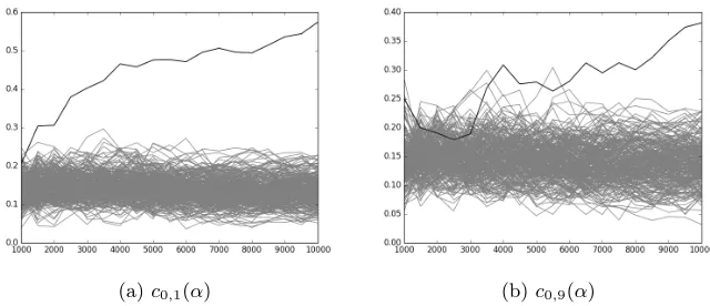
(a)c0,1(α) (b)c0,9(α)

Fig. 1.Correlation ofci,j(α) vs # of traces. The correct value ofαis shown in black.

event is 2−12_{. But sinceB}

s−1((K1, . . . , Ks−1)) is a subsum ofBs((K1, . . . , Ks)),

the probability of Bs(K1, . . . , Ks))≥ 2s

b is larger than 1₂ if we already know that Bs−1((K1, . . . , Ks−1)) ≥ s−₂1

b. We compute an approximation of this probability by a simulation of normally distributed random variables. We get

P

Bs((K1, . . . , Ks))≥

_s

2

bforall s= 16,15, . . . ,5

≈0.15.

6

Experiments

Experimental Setup Our setup consists of an AES-128 based software imple-mentation running on an Atmel ATMEGA328P-PU. The S-Boxes are realized as lookup tables and stored in the program memory of the ATMEGA. The S-Boxes are masked using the method presented in [AG01]. This masking is known to be not leakage-free, and as shown in [CFG+_{11,MME10], also Canright} S-Boxes [Can05] are susceptible to correlation attacks. Hence we anticipate that our results are representative. Moreover, the masking used [AG01] is straightfor-ward to implement. The ATMEGA was setup on a custom prototype board, and powered by a lab-grade power supply at 3.3 Volt. We used a LeCroy HDO6104 to record the power consumption of the ATMEGA with a resistor against ground. We recordedN traces of AES-128 encryption. The plaintext was chosen at ran-dom, and we attacked the masked subbytes procedure of the first AES round.

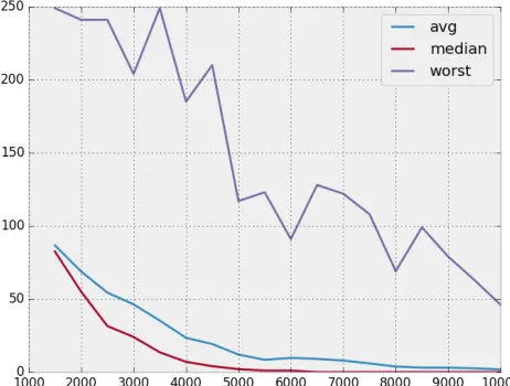
Fig. 2.Number of Traces vs. Ranking Positions ofci,j(α) for correctα.

Practical Results We recorded 10000 traces with randomly generated plain-text values. Our implementation follows closely [MME10] and we compute the correlation w.r.t. each possible value of oneCi,j,α,t. Figure 3a shows the

result-ing correlation of C0,1,α,t for one AES round, i.e. in our setup t= 0, ...,25809.

Correlation peaks at the end of the S-Box for the correct value are clearly visible. However a correlation peak is not apparent for every pair of key byte positions i, j; for example considering the correlation valuesC9,11,α,t as depicted in

and 10000 traces are as shown in Figure 4a and 4b. If more traces are available, the correlation valuesci,j(α) for the correct value αbecome very distinct from

those for incorrect values of α, as illustrated in Figure 1a and Figure 1b. For N = 10000, the correct value of αoften shows on rank 1, but there are some outliers. ForN = 2500, there are few rankings with position 1.

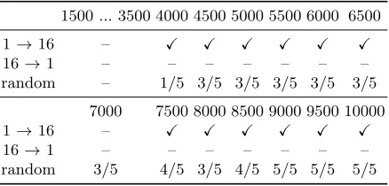
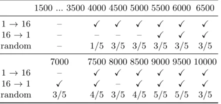
Table 3.Full Key Recovery forW = 1500 using Algorithm 1 (Variant I).

1500 ... 3500 4000 4500 5000 5500 6000 6500

1→16 – X X X X X X

16→1 – – – – – – –

random – 1/5 3/5 3/5 3/5 3/5 3/5

7000 7500 8000 8500 9000 9500 10000

1→16 – X X X X X X

16→1 – – – – – – –

random 3/5 4/5 3/5 4/5 5/5 5/5 5/5

For Variant II of Algorithm 1 one needs to choose appropriate input val-uesg2,· · · , g16. This requires prior knowledge about the quality of the rankings ci,j(α). If such knowledge is not available, appropriate values could also be

esti-mated by manual analysis of the rankingsci,j(α) and/or by visual inspection of

Ci,j,α,t. For example the comparison of Figure 3a and Figure 3b indicates that

forc0,1(α) the ranking for the correct value of αis very likely at one of the top positions, whereas for c9,11(α) this is likely not the case. On the other hand, Variant I of Algorithm 1 requires no prior knowledge at all. Also, if Variant I succeeds, we can always choose the boundgs+1in stepsfor Variant II in such a way that the choice of Variant I is simulated. This is why we have here chosen to implement Variant I of the algorithm.

As mentioned in Section 3, the success of the algorithm depends on the order in which the next key byte position is chosen, the parameter W of candidates that are kept in each iteration, and of course the number of available tracesN. As mentioned in Section 2, in particular the order of choosing the next key byte position is important, as the next example illustrates:

Example 1. For simplicity, suppose we have only a key consisting of three bytes, and suppose one key byte can take only value 0 or 1. Letci,j(α) be as follows:

c0,1(0) = 0.4 c0,1(1) = 0.1 c1,2(0) = 0.4 c1,2(1) = 0.1 c0,2(0) = 0.1 c0,2(1) = 0.8

(a)C0,1,α,t (b)C9,11,α,t

Fig. 3.CorrelationCi,j,α,tfor each timepointtwithin one trace. The correct value of αis denoted in black.

(a)N = 10000 (b)N = 2500

Fig. 4.Ranking positions for correctα.

(a)N = 10000 (b)N = 2500

Algorithm 1 terminates with the setS3={100,011}. Note also that Algorithm 1 is nondeterministic in general: If we setW = 1 in the second step during the run with order 0<1 <2, we have B((00)) = B((11)) = 0.4, and it is open which partial key to keep.

We executed Algorithm 1 forN = 1500 up toN = 10000 in steps of 500 traces, and for bothW = 1500 and W = 10000. As for the dependency on the order, we considered the natural order of starting at key byte position 1 and moving upward to position 16 (denoted by 1→16 in the following), the reverse order of starting at position 16 and moving down to 1 (denoted by 16→1), and on five randomly chosen orders for each value ofN. Table 3 and Table 43 show results

Table 4.Full Key Recovery forW = 10000 using Algorithm 1 (Variant I).

1500 ... 3500 4000 4500 5000 5500 6000 6500

1→16 – X X X X X X

16→1 – – – – X X X

random – 1/5 3/5 3/5 3/5 3/5 3/5

7000 7500 8000 8500 9000 9500 10000

1→16 – X X X X X X

16→1 X X – X X X X

random 3/5 4/5 3/5 4/5 5/5 5/5 3/5

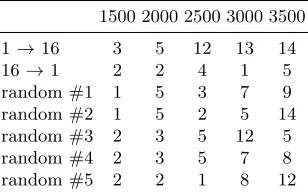
for the full recovery of the key forN = 1500...10000 and the various orders. As one can see, the full key is in the computed set with good probability if at least 4000 traces are available. The probability can be increased, if a larger parameter W = 10000 is chosen. For less than 4000 traces, Table 5 shows the maximum number of correctly recovered key bytes in the computed set. For example, when choosing the order 1 → 16, then in the case of 2500 traces, the computed set contains a key where 12 key bytes are correctly identified. In other words, the entropy is significantly reduced, and it is not difficult to devise an algorithm that exploits the fact that one can assume that a certain amount of key byte position are correctly identified.

In order to further interpret these results, we investigated the distribution ci,j in α for all (i, j). For each (i, j) we computed the expected value as well

the standard deviation, which were very similar. Figure 5a and Figure 5b show histograms of all 255·120ci,jwith incorrect valueαforN= 10000 andN = 2500,

respectively. Expected value and standard deviation are 0.139±0.0374 forN = 10000 and 0.146±0.0363 forN = 2500. As derived above, we expect a theoretical bound b−_σa ≈ p

2 ln(2) ≈ 1.2. This is the smallest value b, for which we can

3

expect that the evaluation function B succeeds. For our experimental data we yield b−_σa =0.336_0.0374−0.139 ≈5.3 forN = 10000 andb−_σa = 0.195_0.0363−0.146 ≈1.3 forN = 2500. Apparently, the parameters forN = 2500 are very close to the theoretical threshold. This fits with our theoretical observations in previous sections and the experimental data. Aside from the above results, we also experimentally verified our findings using a hardened security controller with a hardware based AES implementation, and the results were comparable. However, we refrain from providing more specific data here.

7

Related Work

Suppose we are given a key K1, ..., Kn withn independent subkeys, and a side

channel attack yields for each Ki ranks for possible key values. Using these

ranks, one can define a probability measurement function for each subkey. The key enumeration problem [VCGRS13] is then to enumerate complete keys from the most probable to the least probable one, in order to find the key of a device as quickly as possible. A direct solution is to enumerate all possible keys, compute their probability (multiplying the probabilities of the subkeys) and then sort all keys according to their probability. As this is infeasible in practice, more efficient algorithms have been proposed [VCGRS13].

In our scenario, we do not have ranks (resp. probability measurement func-tions) for all sixteen Ki. Rather, we obtain 120 ranks for each Ki ⊕Kj for

1 ≤ i, j ≤ 16. Our task is to reconstruct the key from these values. Algo-rithms that solve the key enumeration problem are thus not directly applica-ble. One naive way to still apply existing key search algorithms in our scenario would be to (1) select a number of Ki ⊕Kj with their ranks which have a

low remaining entropy, i.e. selectK1⊕K2, K2⊕K3, . . . , K15⊕K16. (2) recover K1⊕K2, K2⊕K3, . . . , K15⊕K16 using an efficient key enumeration algorithm, and for each candidate (3) search among the remaining 256 possibilities for the correct key.

Note that it is not clear how to effectively selectKi⊕Kj. One could for

ex-ample simply takeK1⊕K2, K2⊕K3, . . . , K15⊕K16. How to assess the leakage then? The problem of key ranking [GGP+15,MOOS15,MMOS16] is concerned with quantifying the time complexity required to brute force a key given the leakages, especially if the number of keys to enumerate is beyond practical com-putational limits. Applying e.g. the algorithm of [MMOS16] for our test set of traces with N = 4000 when we interpret K1⊕K2, K2⊕K3, . . . , K15⊕K16 as our key, the estimated rank is approximately 250_{. However with our algorithm} we are able to recover the actual AES key within less than two minutes (cf. Table 3). Directly recovering the key (and not Ki⊕Kj) by making use of all

Ki⊕Kj was the motivation for our algorithm. We anticipate however, that by

either employing voting techniques [Bog08] or by a more sophisticated choice of Ki⊕Kj and repeating steps (1)-(3) one could obtain similar results as with our

Table 5.Partial Key Recovery forW = 1500 using Algorithm 1 (Variant I).

1500 2000 2500 3000 3500

1→16 3 5 12 13 14

16→1 2 2 4 1 5

random #1 1 5 3 7 9

random #2 1 5 2 5 14

random #3 2 3 5 12 5

random #4 2 3 5 7 8

random #5 2 2 1 8 12

In [MS16] the attack of [MME10] is generalized into Moments-Correlating Collision DPA. There, moments are correlated with samples rather than mo-ments with momo-ments, as done in the original attack. Using that, they derive a measure Nsr (equation 1 in [MS16]) that provides a metric to quantify the

number of measurements needed to perform a key recovery with a given success rate. Note however that this measure quantifies the leakage w.r.t. Ki⊕Kj. As

seen in the experiments, the leakage can be quite unsteady, i.e. the correct value of αis in the lower ranks for some i, j, but for other combinations the rank is much higher. Here we provide an algorithm that still works in this scenario and reveal the correct key, and our measureτ thus gives a indicates on whether the key can be recovered or not.

8

Conclusion and Future Work

We have shown how to reduce the remaining key entropy of the attack intro-duced by [MME10] by providing a practical, easy-to-implement algorithm. Our theoretical analysis shows that this algorithm exploits the leakage in a natu-ral way. Moreover, we provide a way to assess the leakage of a device w.r.t. the attack, which could be used e.g. in a Common Criteria security evaluation. Our practical evaluation supports the theoretical analysis. In particular we show that using our algorithm, a full recovery of the AES key is possible with only few available traces. That is, the key can be recovered in a setting where no visual clues w.r.t. the correct ranking are available and the attack as described by [MME10] would not have been applicable. A practical comparison with the metric derived in [MS16] remains future work.

References

[AARR03] D. Agrawal, B. Archambeault, J. R. Rao, and P. Rohatgi. The EM Side— Channel(s). InProc. 4th CHES, pages 29–45, 2003.

[AG01] M.-L. Akkar and C. Giraud. An Implementation of DES and AES, Secure against Some Attacks. InProc. 3rd CHES, pages 309–318, 2001.

[BCO04] E. Brier, C. Clavier, and F. Olivier. Correlation Power Analysis with a Leakage Model. InProc. 6th CHES, 2004.

[Bog08] A. Bogdanov. Multiple-Differential Side-Channel Collision Attacks on AES. InProc. 10th CHES, pages 30–44, 2008.

[Can05] D. Canright. A Very Compact S-Box for AES. InProc. 7th CHES., pages 441–455, 2005.

[CB08] D. Canright and L. Batina. A Very Compact “Perfectly Masked” S-Box for AES. InProc. 6th ACNS, pages 446–459, 2008.

[CFG+_{11] C. Clavier, B. Feix, G. Gagnerot, M. Roussellet, and V. Verneuil. Improved}

Collision-Correlation Power Analysis on First Order Protected AES. In Proc. 13th CHES, pages 49–62, 2011.

[CRR03] S. Chari, J. R. Rao, and P. Rohatgi. Template Attacks. InProc. 4th CHES, pages 13–28, 2003.

[GGP+_{15] C. Glowacz, V. Grosso, R. Poussier, J. Sch¨uth, and F. Standaert. Simpler}

and more efficient rank estimation for side-channel security assessment. In Proc. FSE 2015, pages 117–129, 2015.

[GMO01] K. Gandolfi, C. Mourtel, and F. Olivier. Electromagnetic Analysis: Con-crete Results. InProc. 3rd CHES, pages 251–261, 2001.

[KJJ99] P. Kocher, J. Jaffe, and B. Jun. Differential Power Analysis. InProc. 19th CRYPTO, pages 388–397, 1999.

[Koc96] P. C. Kocher.Timing Attacks on Implementations of Diffie-Hellman, RSA, DSS, and Other Systems, pages 104–113. 1996.

[LMV04] H. Ledig, F. Muller, and F. Valette. Enhancing Collision Attacks. InProc. 6th CHES, pages 176–190, 2004.

[MME10] A. Moradi, O. Mischke, and T. Eisenbarth. Correlation-Enhanced Power Analysis Collision Attack. InProc. 12th CHES, pages 125–139, 2010. [MMOS16] D.P. Martin, L. Mather, E. Oswald, and M. Stam. Characterisation and

estimation of the key rank distribution in the context of side channel eval-uations. InProc. 22nd ASIACRYPT, pages 548–572, 2016.

[MOOS15] D. P. Martin, J. F. O’Connell, E. Oswald, and M. Stam. Counting keys in parallel after a side channel attack. InProc. 21st ASIACRYPT, pages 313–337, 2015.

[MS16] A. Moradi and F. Standaert. Moments-correlating dpa. InProc. 2016 TIS Sec. Workshop, pages 5–15, 2016.

[Nat01] National Institute of Standards and Technology. FIPS PUB 197. Advanced Encryption Standard. Technical report, 2001.

[QS01] J.-J. Quisquater and D. Samyde. EMA: Measures and counter-measures for smart cards. InProc. E-smart, pages 200–210, 2001.

[SLFP04] K. Schramm, G. Leander, P. Felke, and C. Paar. A Collision-Attack on AES. InProc. 6th CHES, pages 163–175, 2004.

[SWP03] K. Schramm, T. Wollinger, and C. Paar. A New Class of Collision Attacks and Its Application to DES. InProc. 10th FSE, pages 206–222, 2003. [VCGRS13] N. Veyrat-Charvillon, B. G´erard, M. Renauld, and F. Standaert. An