Fast and Secure Constant-Time Sampling for
Lattice-Based Crypto
Andreas H¨ulsing, Tanja Lange, Kit Smeets
Department of Mathematics and Computer Science
Technische Universiteit Eindhoven, P.O. Box 513, 5600 MB Eindhoven, NL
[email protected], [email protected], [email protected]
Abstract. This paper suggests to use rounded Gaussians in place of dis-crete Gaussians in rejection-sampling-based lattice signature schemes like BLISS. We show that this distribution can efficiently be sampled from while additionally making it easy to sample in constant time, systemat-ically avoiding recent timing-based side-channel attacks on lattice-based signatures.
We show the effectiveness of the new sampler by applying it to BLISS, prove analogues of the security proofs for BLISS, and present an im-plementation that runs in constant time. Our imim-plementation needs no precomputed tables and is twice as fast as the variable-time CDT sam-pler posted by the BLISS authors with precomputed tables.
Keywords:Post-quantum cryptography, lattice-based cryptography, sig-natures, Gaussian sampling, BLISS, constant-time implementations.
1
Introduction
Lattice-based cryptography is a promising candidate for post-quantum cryptog-raphy. A key reason for this – especially from an applied point of view – is that it is known how to construct efficient signature and encryption/key-exchange schemes from lattice-assumptions. As both primitives are needed for many ap-plications this is an advantage as it allows for code reuse and relying on one sort of cryptographic hardness assumptions instead of two. For all other well-established candidate areas of post-quantum cryptography we only know how to construct ef-ficient and confidence-inspiring signaturesor encryption/key-exchange schemes. In this work we take a look at lattice-based signature schemes. The most efficient lattice-based signature scheme with a security reduction from standard lattice problems today is BLISS (Bimodal Lattice Signature Scheme) [11], de-signed by Ducas, Durmus, Lepoint and Lyubashevsky. BLISS is one of the few
This work was supported by the European Communities through the Horizon 2020 program under project number 645622 (PQCRYPTO) and project number 645421 (ECRYPT-CSA). Permanent ID of this document:
post-quantum schemes of which there already exists a production-level imple-mentation. BLISS (or rather its subsequent improvement BLISS-b [10] by Ducas) is available in the open-source IPsec Linux library strongSwan [24].
BLISS builds on Lyubashevsky’s signature scheme [16] which initiated using rejection sampling to make the signature distribution independent of the used secret key. In the most basic version of these schemes, a discrete Gaussian vector is added to a vector that depends on the secret key. The resulting vector follows a discrete Gaussian distribution that is shifted by a vector that depends on the secret key. To avoid leaking the secret key, a rejection step is executed that ensures that the output distribution is independent of the secret key, i.e. the outputs follow again a centered discrete Gaussian distribution.
The use of discrete Gaussian vectors to blind secrets is a very common approach in lattice-based cryptography. However, it is not trivial to sample from a discrete Gaussian efficiently. Over the last few years, many works have been published that deal with efficient sampling routines for discrete Gaus-sians, see e.g. [8,22,11,12,20]. Despite the number of publications, none achieved constant-time sampling. At CHES 2016, Groot-Bruinderink, H¨ulsing, Lange, and Yarom [7] demonstrated that this enables a cache-attack on BLISS which re-covers the secret key after less than 5000 signatures. While the attack is only implemented for two samplers, the appendix of the full version surveys other efficient samplers and shows for each of them that they have similar issues.
In [7], the authors already discuss straightforward approaches for achieving constant-time implementations of discrete Gaussian samplers, such as determin-istically loading entire tables into cache or fixing the number of iterations for some functions by introducing dummy rounds. While such approaches might work for encryption schemes such as [5], signatures require much wider Gaus-sians to achieve security. Hence, the impact on efficiency of applying these coun-termeasures is larger, effectively rendering their use prohibitive.
A different way to deal with such attacks is to complicate the attack. Such a heuristic approach was proposed by Saarinen [23]. However, this approach does not fix the vulnerability, as shown by Pessl [18]; this only makes it harder to exploit it. In consequence, it starts a cat-and-mouse game of attack and fix.
As the name suggests, sampling from a rounded Gaussian is done by sampling from a continuous Gaussian and rounding the result to an integer. The Box-Muller method is an efficient way of computing samples of continuous Gaussians starting from uniformly random numbers, and all steps leading to rounded Gaus-sian samples are efficiently and easily computed in constant time. We present a constant-time implementation of rounded Gaussians suitable for the BLISS-I parameter set and show that it is more than twice as fast as a sampler based on cumulative distribution tables (CDT) as implemented by the authors of BLISS. The CDT sampler uses large precomputed tables to speed up sampling. Note that the CDT sampler is exactly the one that [7] broke at CHES 2016. Using rounded Gaussians brings better speed and better security. Another benefit of rounded Gaussians is that they can use the Box-Muller sampler (see Section4.1) which naturally does not require any precomputed tables, hence can work with a small code base, and furthermore is extremely easy to implement.
We conclude our work with our second theoretical contribution – a proof that using rounded Gaussians, sampled using our Box-Muller implementation is secure. For this we provide a detailed analysis of the new sampler. We study the difference between (perfect) rounded Gaussians and implementations with finite precisionpusing statistical distance and R´enyi divergence. We also com-pare the asymptotic results using these different measures. We instantiate the calculation for BLISS parameters and the precision achieved by our Box-Muller implementation to derive bounds on the allowable number signatures per key pair.
Related work. Rounded Gaussians are not a new distribution, in fact they have been used in the initial proposals for learning with errors, but were re-placed by discrete Gaussians to make proofs and protocols easier (the sum of two discrete Gaussians is a discrete Gaussian). See, e.g. Regev [21, p.90] for an overview of distributions and [9] for an analysis of wrapped rounded Gaus-sians. Encryption schemes can be secure with narrow non-Gaussian distributions (NTRU/Frodo/New Hope) but signatures are much harder to protect, need much wider distributions (larger parameterσ), seemed to need discrete Gaussians, and so far were analyzed only for discrete Gaussians.
After a first version of our paper was circulated we became aware of a recent paper by Micchiancio and Walter [17] which has a new proposal to perform sampling of discrete Gaussians in constant time. The target of our paper is very different: Showing that rounded Gaussians can efficiently be sampled in constant time and that their use in signature schemes is safe.
2
Preliminaries
Vectors, considered as column vectors, will be written in bold lower case let-ters; matrices will be written in upper case bold letters. For a vector a = (a1, a2, . . . , an) ∈ Rn, the Euclidean norm is defined by kak=p(Pni=1a
2
i).
The ∞-norm is defined by kak∞ = max (|a1|,|a2|, . . . ,|an|). The Hamming
weight wt(a) is the number of non-zero positions in a. For two vectors a = (a1, a2, . . . , an) and b = (b1, b2, . . . , bn), both in Rn, denote the inner product byha,bi=Pn
i=1aibi.
In this paper we will be concerned with (discrete) probability functions. For
a distribution h, we denote by x←−$ hthat x is sampled according toh. For a
setS we denote bys←−$ S that s∈S is sampled uniformly at random fromS. Many lattice-based schemes use rejection sampling to massage one distri-bution to fit another. The followingm-dimensional version which samples once from the provided distribution and outputs with a certain probability depending on both the target distribution and the sample is taken from Lyubashevsky [16].
Lemma 2.1 (Rejection Sampling).LetV be an arbitrary set, andh:V →R
and f : Zm → R be probability distributions. If gv : Zm → R is a family of
probability distributions indexed byv∈V with the property
∃M ∈R:∀v∈V : Pr[M gv(z)≥f(z);z←−$ f]≥1−ε,
then the distribution of the output of the following algorithmA:
1: v←−$ h 2: z←−$ gv
3: output (z,v)with probability minM gf(z) v(z),1
is within statistical distance ε/M of the distribution of the following algorithm
F:
1: v←−$ h 2: z←−$ f
3: output (z,v)with probability 1/M.
Moreover, the probability that Aoutputs something is at least(1−ε)/M.
2.1 Discrete Gaussian Distribution
The discrete Gaussian distribution is based on the continuous Gaussian distri-bution. The definition of the continuous Gaussian distribution, also called the Normal distribution, is given by:
Definition 2.1. The continuous Gaussian distribution overRmcentered at some
v∈Rm with standard deviationσ is defined for x ∈
Rm as the (joint) density
ρm
v,σ(x) =
1
√
2πσ2
m
e−kx−vk
2
Whenv=0, we simply writeρm
σ(x). The definition of the discrete Gaussian
distribution is given by:
Definition 2.2. The discrete Gaussian distribution over Zm centered at some
v∈Zmwith parameterσ is defined forx∈
ZmasDvm,σ(x) =ρvm,σ(x)/ρmσ (Zm),
whereρm
σ (Zm) =
P z∈Zmρ
m σ(z).
Note that the discrete Gaussian distribution is defined over all length-m
integer vectors inZm. However, samples with large entries have negligible prob-ability. Implementations need to provision for the maximal size of coefficients and table-based sampling schemes would require a lot of storage to cover rarely used values and still not cover all possibilities. Therefore, a tail cut τ is used, meaning that only integers in [−τ σ, τ σ]mare sampled. Results about the neces-sary size of the tail cut can be found in [16] and LemmaC.2. In practice, τ is often chosen as√2λln 2, whereλis the security level.
2.2 Lyubashevsky’s Signature Scheme
In 2012 Lyubashevsky [16] designed a signature scheme that uses anm×nmatrix Swith small coefficients as secret key and the following two matrices as public key: a random matrixA∈Zn2q×m and then×nmatrixT=AS modq, where
q is an integer. The matrix A can be shared among all users, but the matrix Tis individual. To sign a message, the signer picks a vectoryaccording to the
m-dimensional discrete Gaussian. Then c=H(Ay modq, µ), whereH(·) is a hash function, and the potential signature vectorz=Sc+y are computed.
The system then uses rejection sampling to shape the distribution of z to a centered discrete Gaussian, i.e., to decide whether to output the candidate signature (z,c). In terms of Lemma 2.1, his the distribution of Sc, gv is the
m-dimensional discrete GaussianDv,σ(z) centered aroundv=Sc, andf is the
m-dimensional centered discrete GaussianDm σ(z).
Because Dm
σ(z) is independent of Sthe signatures do not leak information
about the private key.
2.3 Bimodal Lattice Signature Scheme: BLISS
Ducas, Durmus, Lepoint and Lyubashevsky introduced the Bimodal Lattice Sig-nature Scheme (BLISS) in [11]. BLISS is an improvement of Lyubashevsky’s sig-nature scheme described above. We only cover sigsig-nature generation here as we are focusing on the use of the discrete Gaussian distribution. For a full descrip-tion of BLISS, see AppendixB. BLISS uses a special hash functionH mapping to {c ∈ {0,1}n|wt(c) = κ} for κsome small constant. A simplified version of
the BLISS signature algorithm is given in Algorithm2.1.
Given a messageµ, the signing algorithm first samples a vectoryfrom them -dimensional discrete Gaussian distributionDσm. Then it computes the hashc←
Algorithm 2.1Simplified BLISS Signature Algorithm using matrices
Input: Messageµ, public keyA∈Zn2q×mand secret keyS∈Z m×n 2q Output: A signature (z,c) of the messageµ
1: y←Dm σ
2: c←H(Aymod 2q, µ) //c∈ {0,1}n
, wt(c) =κ,κsmall constant 3: Choose a random bitb∈ {0,1}
4: z←y+ (−1)bSc
5: Output (z,c) with probability 1.Mexp−kSck2
2σ2
coshhzσ,Sc2i
rejection sampling according to Lemma 2.1, i.e., it outputs the signature (z,c)
with probability 1.Mexp−kSc2σk22
coshhzσ,Sc2 i
, where M is some fixed positive real constant that is set large enough to ensure that this probability is at most 1 for all choices of c. If the signature algorithm is unsuccessful, it restarts with a freshyand continues until a signature is output.
Again, rejection sampling is used to force the distribution of the outputzto be that of a centered Gaussian distribution (i.e., to be independent ofSc).
The bulk of the time in one round of the signing algorithm using BLISS is spent in the first step in generating m samples from the one-dimensional Gaussian. The number of repetitions depends on M and the size ofSc.
Bound on kSck. The parameter σ of the discrete Gaussian distribution, the size of Sc, and the rejection rateM control how much the distributions of the target distribution Dm
σ and the input distribution overlap, i.e., how smallεcan
be achieved. For BLISS the input distribution is a bimodal Gaussian distribution 0.5(Dm
−Sc,σ+DmSc,σ). BLISS’ authors show that rejection sampling can be used
without error, i.e., ε= 0 is possible in Lemma 2.1 with resonable choices of σ
andM. In later sections we require an upper bound on kSck for proofs. In [11] a new measure Nκ(X) ofS, adapted to the form ofcis presented.
Definition 2.3. For any integerκ,Nκ:Rm×n→R is defined as:
Nκ(X) = max I⊂{1,...,n},#I=κ
X
i∈I
max
J⊂{1,...,n},#J=κ
X
j∈J
Wi,j
,
whereW=XT ·X∈Rn×n.
With this definition, the authors of [11] show that for anyc∈ {0,1}n with
wt(c) ≤ κ, we have kSck2 ≤ N
κ(S) [11, Proposition 3.2]. In addition to the
use of bimodal Gaussians, this upper bound lowers the parameterσby a factor ≈√κ/2 compared to [16].
3
Rounded Gaussian Rejection Sampling
In this section we discuss the applicability of therounded Gaussian distribution
def-inition of the rounded Gaussian distribution, we provide proofs showing that it can be used to replace the discrete Gaussian distribution in Lyubashevsky’s signature scheme and in BLISS. We show the analogies between the rounded Gaussian distribution and the discrete Gaussian distribution and we point out where the security reductions differ when rounded Gaussians are used in place of discrete Gaussians. In practice, the most important question is how the prob-ability in Step5 in Algorithm2.1needs to change if yis sampled according to the rounded Gaussian distribution instead of the discrete Gaussian distribution. Note, again, that this step determines the rejection rate, i.e. how many times the algorithm needs to restart sampling fresh randomness.
We follow the reasoning from [16] and [11] very closely to show the applica-bility of the rounded Gaussian distribution to the BLISS signature scheme. The main difference is that the definition of rounded Gaussians requires integrals over an interval of length 1, while the definition of discrete Gaussians requires a division by the probability mass at all integers. We essentially have to prove the same lemmas that were shown for discrete Gaussians in [16] and [11] for rounded Gaussians. In the end closely analogous results hold but the analysis turns out far more complicated than in the discrete Gaussian setting because we have to deal with bounding integrals.
3.1 Rounded Gaussian Distribution
We now formally define the rounded Gaussian distribution. Intuitively, the rounded Gaussian distribution is obtained by rounding samples from a continuous Gaus-sian distribution to the nearest integer xi. To compute the probability at an
integer xi, we compute the integral over the interval (xi−12, xi+12].
Definition 3.1. The rounded Gaussian distribution overZmcentered at some
v∈Zmwith parameter σ is defined forx∈
Zm as
Rvm,σ(x) = Z
Ax
ρmv,σ(s)ds= Z
Ax
1
√ 2πσ2
m exp
−ks−vk2
2σ2
ds,
whereAx denotes the area defined by
x1−12;x1+12
× · · · ×
xm−12;xm+12
.
We point out that this gives us vol(Ax) = 1, since the volume of this area is equal to|(x1+12)−(x1−12)| · · · |(xm+12)−(xm−12)|. Note that the
parame-ter σ in the definition above is the standard deviation of the underlying con-tinuous Gaussian and not the standard deviation σ0 of the rounded Gaussian distribution, which is given byσ0=
q
σ2+ 1
12. The proof of this, the proof that
the distribution above is a probability density function, and that it is centered atv, can be found in AppendixA.
3.2 Using Rounded Gaussians in Lyubashevsky’s Scheme
The following lemma states that the centered rounded GaussianRm
σ(z) and the
shifted rounded Gaussian Rv,σ(z) are almost always close, and Theorem 3.1
applies it to the rejection-sampling Lemma 2.1.
Lemma 3.1. For any v∈Zm, ifσ=ω(kvk √
logm), then
PrhRmσ(z)/Rmv,σ(z) =O(1);z←−$ Rmσi= 1−2−ω(kvk √
logm).
This is proven in AppendixC.
Theorem 3.1. Let V be a subset of Zmin which all elements have norms less
thanT,σ be some element inR such that σ=ω(T√logm), andh:V →Rbe a probability distribution. Then there exists a constant M =O(1)such that the distribution of the following algorithm A:
1: v←−$ h 2: z←−$ Rm
v,σ
3: output (z,v)with probability min Rmσ(z)
M Rm v,σ(z),1
is within statistical distance 2−ω(logm)/M of the distribution of the following
algorithmF:
1: v←−$ h 2: z←−$ Rm
σ
3: output (z,v)with probability 1/M.
Moreover, the probability thatAoutputs something is at least(1−2−ω(logm))/M.
Proof. The proof of this theorem follows immediately from Lemma3.1and the
general “rejection sampling” Lemma2.1. ut
This theorem looks the same for rounded Gaussians and for discrete Gaus-sians; see AppendixC.1for a detailed comparison of the results.
3.3 Using Rounded Gaussians in BLISS
In Section 3.2 we have shown that we can use the rounded Gaussian distribu-tion in the rejecdistribu-tion sampling scheme by Lyubashevsky [16]. Now we need to show that we can apply the rounded Gaussian distribution to BLISS. BLISS randomly flips a bit to decide on adding or subtractingSc, i.e., for fixedSc,z∗ is distributed according to the bimodal rounded Gaussian distributiongSc(z∗) =
1 2R
m
Sc,σ(z∗) +
1 2R
m
−Sc,σ(z∗). To avoid leaking any information on the secret key
S the scheme requires rejection sampling to change the bimodal Gaussian to a centered Gaussian f(z∗) = Rm
σ(z∗). The probability to accept is given by
pz∗=f(z∗) /M gSc(z∗) , where again M is chosen minimal such that this prob-ability is≤1.
For anyz∗∈Zm, we have
Pr[z=z∗] =12RmSc,σ(z∗) +12Rm−Sc,σ(z∗)
=12√ 1
2πσ2
m R
Az∗exp
−kx−2σSc2k2
+ exp−kx+2σSc2k2
dx
= exp−kSc2σk22
1
√
2πσ2
mR
Az∗exp
−k2xσk22
coshhxσ,Sc2 i
dx
≥exp−kSc2σk22
1
√
2πσ2
m R
Az∗exp
−k2xσk22
dx,
(1)
where the last inequality comes from the fact that cosh(x)≥1 for any x. Note that the last inequality cannot be used to compute M and is only needed to estimate an upper bound for it.
The desired output is the centered rounded Gaussian distributionf(z∗), since we need the centered property to avoid leaking S. Thus by Theorem 3.1, we should accept the samplez∗ with probability:
pz∗=f(z∗)/(M gSc(z∗))
=
1
√
2πσ2
m R
Az∗exp −kxk
2/(2σ2)
dx
Mexp (−kSck2/(2σ2))√1 2πσ2
m R
Az∗exp (−kxk
2/(2σ2)) cosh (hx,Sci/σ2)dx
.
To compute a bound on M, we use the last inequality from Equation (1). This leads to the following upper bound:
pz∗=
R
Az∗exp −kxk
2/(2σ2)
dx
Mexp (−kSck2/(2σ2))R
Az∗exp (−kxk
2/(2σ2)) cosh (hx,Sci/σ2)dx
≤
R
Az∗exp −kxk
2/(2σ2)
dx
Mexp (−kSck2/(2σ2))R
Az∗exp (−kxk
2/(2σ2))dx
= 1/(Mexp −kSc∗k2/(2σ2) ).
NowM needs to be chosen large enough such thatpz∗ ≤1. Note again that the last inequality can only be used to estimateM, and not to define the probability. It suffices that
M = exp 1/(2α2)
,
where α > 0 is such that σ ≥αkSck. We can use the upper bound kSck2 ≤
Nκ(S) as in Definition 2.3 to put M = exp(Nκ(S)/2σ2); here κ denotes the
sparsity ofcin Algorithm2.1.
It would be very inefficient if the rejection step needed to compute the in-tegrals in Equation (1). When using discrete Gaussians the expressions simplify to the expression 1 Mexp −kSck2/(2σ2)
cosh hz,Sci/σ2 given in Algo-rithm2.1. To avoid computing the integrals when using rounded Gaussians we look at the maximum and minimum value of 1cosh hx,Sci/σ2 on the area
Az∗. We picky1∈[−1
2, 1 2]
m such thaty
1 minimizes 1/cosh hz∗+y1,Sci/σ2
andy2∈[−12,12]msuch thaty2maximizes 1/cosh hz∗+y2,Sci/σ2
us
1
Mexp−kSc2σk22
coshhz∗+y1,Sci σ2
≤
f(z∗)
M gSc(z∗)≤
1
Mexp−kSc2σ2k2
coshhz∗+y2,Sci σ2
.
In the next formulas we use (Sc)i to denote theith element ofSc matching
the notation of theith element ofz∗.
We first determine when cosh((xi·(Sc)i)/σ2), xi∈[z∗i−
1 2, z
∗
i+
1
2] is maximized
and when it is minimized.
max
xi∈[z∗ i− 1 2,z ∗ i+ 1 2]
cosh(xi·(Sc)i)/σ2) =
cosh(((z∗i −1
2)·(Sc)i)/σ 2) ifz∗
i <0,
cosh(((z∗i +12)·(Sc)i)/σ2) ifz∗i ≥0.
and
min
xi∈[z∗
i−12,zi∗+12]
cosh(xi·(Sc)i)/σ2) =
cosh(((zi∗+12)·(Sc)i)/σ2) ifz∗i <0,
cosh(0) = 1 ifz∗i = 0,
cosh(((zi∗−1
2)·(Sc)i)/σ 2) ifz∗
i >0.
Using these definitions, we have that the relative gap between the two func-tions is given by
m Y i=1 1 cosh ((z∗
i ·(Sc)i+y1,i)/σ2)
− 1
cosh ((z∗
i ·(Sc)i+y2,i)/σ2)
= m Y =1 1 exp (1/σ2) cosh (z∗
i ·(Sc)i+y1,i)
− 1
exp (1/σ2) cosh (z∗
i ·(Sc)i+y2,i)
≤exp − 1 σ2 · m Y i=1 1 cosh zi∗+12
·(Sc)i
− 1
cosh zi∗−1 2
·(Sc)i
≤exp − 1 σ2 1 2 m ,
where the last inequality uses that
max
z∗ i∈Z
1 cosh zi∗+12
·(Sc)i
− 1
cosh zi∗−1 2
·(Sc)i
< 1 2.
This means that the relative error is<(1/2)m. In other words, we have
M−1exp
kSck2
2σ2 cosh
−1
hz∗,Sci
σ2
−2−m
< f(z
∗)
M gSc(z∗)
M−1exp
kSck2
2σ2 cosh
−1hz∗,Sci
σ2
+ 2−m
.
The dimensionmis significantly larger than the security level (see TableB.1
for suggested parameters) and thus the summand 1/2mis negligible and we can use the same constant for rejecting as in the original BLISS signature algorithm (Algorithm2.1), namely 1.Mexp−kSc2σ2k2
coshhz∗σ,Sc2 i
3.4 BLISS Security Reduction
The security proof as given in [11] works for the rounded Gaussian distribution with very little tweaking. This is due to the changes made in the proofs in Section 3.2and AppendixC. All statements follow through when replacing the discrete Gaussian distribution with the rounded Gaussian distribution. We do not need to adjust the proofs for [11, Lemma 3.3, 3.5]. The proof for [11, Lemma 3.4] uses σ ≥ 3/√2π which comes from [16, Lemma 4.4]. Our corresponding result is LemmaC.2which requiresσ≥p
2/π. Next to that, we need to adjust the definitions of f(z) andgSc(z) as above, such that these match the rounded Gaussian distribution.
4
Practical Instantiation
In this section we discuss how we can implement a sampler for the rounded Gaussian distribution. A very efficient and easy way to generate samples from the continuous Gaussian distribution is based on the Box-Muller transform. We state the algorithm and discuss an early rejection technique to prevent the com-putation of values which would later be rejected due to the tail cut. Finally, we analyze the output precision required for an implementation of the rounded Gaussian distribution.
4.1 Box-Muller Transform
We begin by reviewing the Box-Muller transform [6] which is used to create centered Gaussian distributed numbers with standard deviation σ = 1 from uniform random distributed numbers. The algorithm is given as Algorithm 4.1
below.
Algorithm 4.1Box-Muller Sampling Input: Two uniform numbersu1, u2∈(0,1]
Output: Two independent centered (continuous) Gaussian distributed numbersx1, x2 with standard deviationσ= 1
1: a←√−2 lnu1 2: b←2πu2
3: (x1, x2)←(acosb, asinb) 4: return (x1, x2)
The following was already shown in [6].
Theorem 4.1. Let u1, u2 be samples from the uniform distribution over R∩ (0,1] then the two outputs of Algorithm 4.1 are independent samples from a (continuous) Gaussian distribution, centered at zero and with standard deviation σ= 1.
4.2 Sampling Rounded Gaussians
We can now use the Box-Muller transform to create an algorithm for sampling according to the rounded Gaussian distribution. For applying rounded Gaussians to the signature scheme of BLISS, we need centered rounded Gaussians with parameterσ. This is done by scaling the outputxifori= 1,2 of the Box-Muller
sampling schemezi0 =xi·σand then rounding the nearest integerzi=bzi0e.
This leads to Algorithm4.2for sampling numbers according to the rounded Gaussian distribution. For ease of notation we assume thatm= 2nis even.
Algorithm 4.2Rounded Gaussian Sampling
Input: The required number of samplesm= 2nand parameterσ
Output: m independent rounded Gaussian distributed numbers z0, . . . , z2n−1 with parameterσ
1: fori= 0ton−1do
2: Generate two uniform random numbersu1, u2 3: x1, x2←BoxMuller(u1, u2)
4: z2i← bx1·σe
5: z2i+1← bx2·σe
6: end for
7: return (z0, . . . , z2n−1)
Early Rejection. As the targeted schemes use a tail cut, samples greater than the tail cut have to be rejected. For applications in lattice-based cryptography, including our use-case, this is unnecessary. The tail cut is chosen such that the probability mass at the tails is negligible and hence, sampling these values is roughly as likely as correctly guessing the secret key.
However, if applications use a tail cut with recognizable probability mass on the tails, rejections can be implemented almost for free. The magnitude of the outputs of Algorithm 4.1 is bounded by a since sinb,cosb ∈ [−1,1]. We only sample values above a given threshold for largeu1. More specifically, if we use a
tail cutτ σ, we will rejectσ√−2 lnu1> τ σat a later point. Turning this around,
we will not reject values computed from a uniformly random sampleu1for which
u1<exp(−τ2/2)
holds. Therefore, we can already reject initial samples from the uniform distri-bution with no computations and only one comparison. We only need to pre-compute exp(−τ2/2) once for fixed tail cutτ.
5
Code Analysis and Benchmarks
floating point precision and allowable number of signatures. We end with timings and a comparison to the BLISS CDT sampler.
5.1 Implementation Details
We have used the C++ vector class library VCL by Fog [13] for the implemen-tation of the Box-Muller sampling and the rounded Gaussian sampling. This library offers optimized vector operations for integers, floating point numbers and booleans. We useVec8d, which are vectors with 8 elements of double float-ing point precision. This means that we are only limited by the maximum size of thedoubletype, i.e. values of at most 53 bits of precision.
According to [13], the trigonometric and logarithmic functions in VCL have constant runtime, i.e. there is no timing difference dependent on the input. This makes the library ideal for constant-time implementations.The square-root func-tionsqrt(·)takes constant time, unless all 8 inputs are in{0,1}, which can lead to a timing difference for the square root. However, this is unlikely to happen: thesqrtfunction is applied to 2 lnu1 and the logarithm function is strictly
pos-itive and thus the case of input 0 cannot appear; the probability of sampling 8 consecutive valuesu1ithat all would evaluate 2 lnu1i= 1 is negligible, since each
u1i is sampled from (0,1] with 53 bit precision, making this an event of
proba-bility at most 2−8·53. Therefore we have chosen not to circumvent this problem in the implementation, even though one could also sacrifice a vector entry and force it to have a nontrivial square root computation.
Computing with floating-point numbers causes a drop in precision. While Fog states that operations in VCL lose at most one bit of precision with exception of several explicitly mentioned functions that can lose up to two bits of precision such as the trigonometric functions, a more careful analysis of the code shows that other operations keep (close to) the exact precision.
Implementing Algorithm4.2 on top of VCL is only a few lines of code and the data paths are short (see the code listing in Appendix F). The input of the code has 53 bits of precision and we loose at most 5 bits of precision, i.e. the output of the code has at leastp= 48 bits of precision.
Remark 1. We were asked how to round floating point numbers in constant time. While VLC almost trivially rounds the entire vector in constant time, a bit more care is necessary if one wants to implement this on single values. To round|A|<251 compute
(A+ (252+ 251))−(252+ 251)
in two arithmetic instructions or use assembly instructions.
5.2 Considerations Regarding the Precision
precision. This raises the question of how much a low-precision table can skew the distribution and whether this can lead to attacks. Similarly, floating-point computations, such as in our sampler, can slowly degrade precision.
An error in the computation ofyresults in a valuey0 which might be slightly larger or smaller thany. The magnitude of the error depends on the size of the value, e.g., values close to 0 have higher precision than larger values; in general the error of yis bounded by|y|2−p.
When computing rounded Gaussians, most errors are insignificant because most erroneous values still get rounded to the correct integer. However, errors occurring close to the boundaries of the intervals [z − 1
2, z+ 1
2] can lead to
wrong outputs. The interval of values that can possibly round to z is given by [z−1
2−el, z+ 1
2+er), where the left boundary error satisfies|el| ≤2
−p z−12
and the right boundary error satisfies|er| ≤2−p
z+12
.
We define success for the attacker to mean that he breaks the signature scheme or that he manages to distinguish between the implementation with precision pand a perfect implementation.
Most papers use the statistical distance (DefinitionE.1) to study the relative difference between two distributions. In [1] the authors showed that studying the R´enyi divergence between the distributions can lead to better and tighter estimates.
In this section we work with the known precision p = 48 for our imple-mentation and using the parameters for BLISS-I [11], we determine how many signatures an adversary A can observe before the R´enyi divergence between the ideal implementation and the practical implementation becomes larger than some small constantc; this means, his chance of breaking the system is as most
c times as high compared to the ideal implementation.
We also provide an analysis of the asymptotic behavior of the precision p
compared to the standard deviationσ, the lengthmand the number of signa-turesqsgenerated. The computations can be found in AppendixE. These results
are naturally less tight because we prioritize readable formulas over best approx-imations. Accordingly, better results are obtained using numerical computations once one settles on concrete parameters. The asymptotic analysis is helpful in determining which distance or divergence to use.
To analyze the allowable number of signatures qs before an attack could
possibly distinguish the distributions, we look at theR´enyi divergence of order
∞as given in [1]:
Definition 5.1. For any two discrete probability distributions P and Q, such that Supp(P)⊆Supp(Q), the R´enyi divergence of order∞is defined by
RD∞(P ||Q) = max
x∈Supp(P)
P(x)
Q(x).
In BLISS using rounded Gaussians generated with Algorithm4.2we publish
m independently sampled integers distributed according to the 1-dimensional rounded Gaussian distribution R1σ to obtain an m-dimensional vector in Rmσ.
learn a vector of lengthmqswith entries from the (imprecise) real-world sampler
Rσ01. We want to determine the probability that an attacker can distinguish between a vector sampled fromRmqs
σ andR0 mqs
σ .
By the probability preservation property (Lemma E.2) of the R´enyi di-vergence, any adversary A having success probability on the scheme imple-mented with imprecise rounded Gaussian sampling has a success probability
δ≥/RD∞(R0σmqs ||Rmqσ s) on the scheme implemented with the perfect rounded
Gaussian. For a target success probability we have to chooseδ≤/exp(1) to have only a small, constant loss in tightness.
We need mqs samples to create qs signatures. By the multiplicative
prop-erty of the R´enyi divergence (Lemma E.1), we have RD∞(R0σmqs || Rmqσ s) ≤
RD∞(R0
1
σ || Rσ1)mqs, so we can relate the divergence of the one-dimensional
distributions to the mqs dimensional one. The formula becomes
RD∞(R0
1
σ ||R
1
σ) =
max
z∈Supp(R01
σ) (
Z z+12+er
z−1 2−el
1 √
2πσ2e
−x2/(2σ2)
dx
, Z z+12
z−1 2
1 √
2πσ2e
−x2/(2σ2)
dx
)
.
The BLISS-I [1] parameters are τ = 5.4, σ = 541, m = 2n = 1024 and
= 2−128and we work with floating point precisionp= 48. Parameters for other BLISS versions are provided in TableB.1. We compute RD∞numerically for the 1-dimensional case with Pari-GP with precision 200 digits, giving RD∞(R01σ ||
R1
σ) = 1.0000000000207622075416975795530100547. Recall we want RD∞(R01σ ||
R1
σ)qs≤exp(1).
We getqs= 225gives 2.0408859832090826613407952767416874636<exp(1).
This means that we can create 225 signatures, i.e., 1 signature/min for over 60
years, securely with one key pair. Note also that the choice of exp(1) is kind of arbitrary and other constants would be suitable as well. Moreover, provable security continues to degrade slowly after these 225signatures. As far as we know, no attack is known that would use the distinguishability of the distributions.
5.3 Timings
Another property that needs to be compared between the rounded Gaussian distribution and the discrete Gaussian distribution is the time it takes to generate one signature. We compare our implementation to the CDT implementation from
http://bliss.di.ens.fr/ which is a proof-of-concept, variable-time sampler for discrete Gaussians.
Our implementation starts by drawing random bits from/dev/urandomand then expanding them using ChaCha20 [3] to 8192 bytes of data. From that 128 vectors of 8 53-bit floating-point variables are initialized with randomness, corre-sponding to the initialuivalues in Algorithm4.1. The rest of the implementation
follows closely the description of that algorithm.
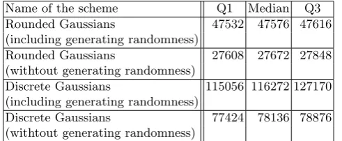
Both implementations have been compiled using gcc with -O3. The bench-marks have been run on a Haswell Intel(R) chip, i.e. Intel(R) Xeon(R) CPU E3-1275 v3 3.50GHz. All values given in Table 5.1 are given in CPU cycles. We give the quartiles Q1 and Q3 and the median over 10 000 runs to show the statistical stability.
Name of the scheme Q1 Median Q3
Rounded Gaussians 47532 47576 47616 (including generating randomness)
Rounded Gaussians 27608 27672 27848 (withtout generating randomness)
Discrete Gaussians 115056 116272 127170 (including generating randomness)
Discrete Gaussians 77424 78136 78876 (withtout generating randomness)
Table 5.1.CPU cycles analysis for the rounded Gaussian sampling scheme and discrete Gaussian sampling scheme withm= 1024 run on Intel(R) Xeon(R) CPU E3-1275 v3 3.50GHz., stating median and quartiles for 10 000 runs.
In Table5.1 we can clearly see that the rounded Gaussian implementation is significantly faster than the discrete Gaussian implementation; the rounded Gaussian implementation needs noticeably less than half the number of CPU cycles compared to the discrete Gaussian implementation. We can also see that generating the randomness takes a significant part of the total CPU cycle count. While the difference in speed is significant we would like to point out that the implementation we used for the discrete Gaussians is not fully optimized. It is hard to predict how much faster a better implementation would be and how much worse the performance would drop if countermeasures to achieve constant-time behavior were implemented.
Our motivation after [7] was to find an alternative to hard-to-secure discrete Gaussians, even if it wasslowerthan current implementations. Our implemen-tation shows that with less than 40 lines of code rounded Gaussians are at least fully competitive.
References
rather than the statistical distance. InASIACRYPT (1), volume 9452 ofLecture Notes in Computer Science, pages 3–24. Springer, 2015.
2. Wojciech Banaszczyk. New bounds in some transference theorems in the geometry of numbers. Mathematische Annalen, 296(1):625–635, 1993.
3. Daniel J. Bernstein. The ChaCha family of stream ciphers. ChaCha, a variant of Salsa20 [4],https://cr.yp.to/chacha.html.
4. Daniel J. Bernstein. The Salsa20 family of stream ciphers. In New stream ci-pher designs: the eSTREAM finalists, volume 4986 ofLecture Notes in Computer Science, pages 84–97. Springer, 2008.
5. Joppe W. Bos, Craig Costello, Michael Naehrig, and Douglas Stebila. Post-quantum key exchange for the TLS protocol from the ring learning with errors problem. In IEEE Symposium on Security and Privacy, pages 553–570. IEEE Computer Society, 2015.
6. George E. P. Box and Mervin E. Muller. A note on the generation of random normal deviates. Ann. Math. Statist., 29(2):610–611, 1958.
7. Leon Groot Bruinderink, Andreas H¨ulsing, Tanja Lange, and Yuval Yarom. Flush, Gauss, and reload - A cache attack on the BLISS lattice-based signature scheme. In Benedikt Gierlichs and Axel Y. Poschmann, editors, Cryptographic Hardware and Embedded Systems - CHES 2016 - 18th International Conference, Santa Bar-bara, CA, USA, August 17-19, 2016, Proceedings, volume 9813 ofLecture Notes in Computer Science, pages 323–345. Springer, 2016.
8. Johannes A. Buchmann, Daniel Cabarcas, Florian G¨opfert, Andreas H¨ulsing, and Patrick Weiden. Discrete Ziggurat: A time-memory trade-off for sampling from a Gaussian distribution over the integers. In Lange et al. [15], pages 402–417. 9. Alexandre Duc, Florian Tram`er, and Serge Vaudenay. Better algorithms for LWE
and LWR. In Elisabeth Oswald and Marc Fischlin, editors, Advances in Cryptol-ogy - EUROCRYPT 2015 - 34th Annual International Conference on the Theory and Applications of Cryptographic Techniques, Sofia, Bulgaria, April 26-30, 2015, Proceedings, Part I, volume 9056 of Lecture Notes in Computer Science, pages 173–202. Springer, 2015.
10. L´eo Ducas. Accelerating BLISS: the geometry of ternary polynomials. IACR Cryptology ePrint Archive, Report 2014/874, 2014. https://eprint.iacr.org/ 2014/874.
11. L´eo Ducas, Alain Durmus, Tancr`ede Lepoint, and Vadim Lyubashevsky. Lattice signatures and bimodal Gaussians. InCRYPTO (1), volume 8042 ofLecture Notes in Computer Science, pages 40–56. Springer, 2013. full version http://eprint. iacr.org/2013/383.
12. Nagarjun C. Dwarakanath and Steven D. Galbraith. Sampling from discrete Gaus-sians for lattice-based cryptography on a constrained device. Appl. Algebra Eng. Commun. Comput., 25(3):159–180, 2014.
13. Agner Fog. VCL C++ vector class library, 2016. Code and documentation,www. agner.org/optimize.
14. Svante Janson. Rounding of continuous random variables and oscillatory asymp-totics.The Annals of Probability, 34(5):1807–1826, 2006.http://dx.doi.org/10. 1214/009117906000000232.
15. Tanja Lange, Kristin E. Lauter, and Petr Lisonek, editors. SAC, volume 8282 of
Lecture Notes in Computer Science. Springer, 2014.
17. Daniele Micciancio and Michael Walter. Gaussian sampling over the integers: Efficient, generic, constant-time. In Jonathan Katz and Hovav Shacham, editors,
Advances in Cryptology - CRYPTO 2017 - 37th Annual International Cryptology Conference, Santa Barbara, CA, USA, August 20-24, 2017, Proceedings, Part II, volume 10402 of Lecture Notes in Computer Science, pages 455–485. Springer, 2017.
18. Peter Pessl. Analyzing the shuffling side-channel countermeasure for lattice-based signatures. InINDOCRYPT, volume 10095 ofLecture Notes in Computer Science, pages 153–170, 2016.
19. Thomas P¨oppelmann.Efficient implementation of ideal lattice-based cryptography. PhD thesis, Ruhr University Bochum, Germany, 2016.
20. Thomas P¨oppelmann, L´eo Ducas, and Tim G¨uneysu. Enhanced lattice-based sig-natures on reconfigurable hardware. In CHES, volume 8731 of Lecture Notes in Computer Science, pages 353–370. Springer, 2014.
21. Oded Regev. On lattices, learning with errors, random linear codes, and cryp-tography. ACM Conference on Computer and Communications Security, 56(6), 2009.
22. Sujoy Sinha Roy, Frederik Vercauteren, and Ingrid Verbauwhede. High precision discrete Gaussian sampling on FPGAs. In Lange et al. [15], pages 383–401. 23. Markku-Juhani O. Saarinen. Gaussian sampling precision and information leakage
in lattice cryptography. IACR Cryptology ePrint Archive, Report 2015/953, 2015. https://eprint.iacr.org/2015/953.
24. strongSwan. strongSwan 5.2.2 released, January 2015.https://www.strongswan. org/blog/2015/01/05/strongswan-5.2.2-released.html.
25. Tim van Erven and Peter Harremo¨es. R´enyi divergence and Kullback-Leibler di-vergence. IEEE Trans. Information Theory, 60(7):3797–3820, 2014.
A
Rounded Gaussian Proofs
In this section we show that the functionRmv,σ(z) in Definition3.1is a probability
density function (PDF) and that it has meanv =0. Next to that, we need to find out what the standard deviationσ0 is. We note that the parameterσis the standard deviation of the underlying continuous Gaussian and not the standard deviation of the rounded Gaussian.
A.1 Proof of PDF
First we show that the function Rm
v,σ(z) given in Definition 3.1, actually is a
probability density function. A discrete function is a probability density function if and only if the sum over the support equals 1 and it has non-negative output, i.e. in our case:
Rmv,σ(z) is a PDF ⇔ X z∈Zm
Rmv,σ(z) = 1 and Rmv,σ(z)≥0 ∀z∈Zm. (2)
the sum over the support equals 1. First we look into the 1-dimensional case:
P
z∈Z
R1v,σ(z) = P
z∈Z
Rz+12
z−1 2
1
√
2πσ2exp
−(s−v)2
2σ2
ds
=R−∞∞ √ 1
2πσ2exp
−(s−v)2
2σ2
ds
= 1,
where we use that Rb
af(x)dx+
Rc
b f(x)dx=
Rc
af(x)dxin the second equality.
To extend this toRm
v,σ(z) form >1, we first note that the Gaussian samples
are independent of each other. We rewrite the sum from Equation (2):
P
z∈Zm
Rmv,σ(z) = P
z1∈Z
P
z2∈Z
· · · P
zm∈Z
Rmv,σ(z)
= P
z1∈Z
P
z2∈Z
· · · P
zm∈Z
Rzm+12 zm−1
2
· · ·Rz2+12 z2−12
Rz1+12 z1−12
1
√
2πσ2
m ·
exp−ks2−σ2vk2
ds1ds2. . . dsm
= P
z1∈Z
P
z2∈Z
· · · P
zm∈Z
Rzm+12
zm−1 2
· · ·Rz2+12
z2−1 2
Rz1+12
z1−1 2
1
√
2πσ2
m ·
exp
−((s1−v1)2+(s2−v2)2+···+(sm−vm)2)
2σ2
ds1ds2. . . dsm
= P
z1∈Z
P
z2∈Z
· · · P
zm∈Z
Rzm+12 zm−12
· · ·Rz2+12 z2−12
Rz1+12 z1−12
1
√
2πσ2
m ·
exp
−(s1−v1)2)
2σ2
exp
−(s2−v2)2)
2σ2
· · ·exp
−(sm−vm)2)
2σ2
ds1ds2. . . dsm
= P
z1∈Z
Rz1+12 z1−12
1
√
2πσ2
exp
−(s1−v1)2)
2σ2
ds1·
P
z2∈Z
Rz2+12 z2−12
1
√
2πσ2
exp
−(s2−v2)2)
2σ2
ds2· · ·
P
zm∈Z
Rzm+12 zm−1
2
1
√
2πσ2
exp
−(sm−vm)2)
2σ2
dsm
=R∞ −∞
1
√
2πσ2
exp
−(s1−v1)2)
2σ2
ds1·R
∞ −∞
1
√
2πσ2
exp
−(s2−v2)2)
2σ2
ds2· · ·
R∞ −∞
1
√
2πσ2
exp
−(sm−vm)2)
2σ2
dsm
= 1·1· · ·1 = 1,
where we use that all variables are independent in the second to last equality. Thus we have proven that the function from Definition3.1is a probability density function.
A.2 Proof of Mean
mean 0if we start with a continuous Gaussian with mean 0. First we look at the 1-dimensional case. We note that for the 1-dimensional rounded Gaussian with parameterσwe can writeRσ1(i) =Φ
i+1 2 σ
−Φi−12 σ
, whereΦ(x) denotes
the Cumulative Distribution Function (CDF) of the Normal distribution for the valuex, i.e. the continuous Gaussian withv= 0 andσ= 1 for the valuex. For a Gaussian distribution with someσ >1 we useΦ(x/σ) to determine the CDF,
i.e. we normalize the valuexby dividing byσ. Letz←−$ R1
σ. Then we have:
E[z] = limk→∞
k
P
i=−k
i·R1
σ(i)
= limk→∞
k
P
i=−k
i·Φi+12 σ
−Φi−12 σ
= limk→∞ −1
P
i=−k
i·Φi+12 σ
−Φi−12 σ
+ 0 +
k
P
i=1
i·Φi+12 σ
−Φi−12 σ
!
= limk→∞ k
P
i=1
−i·Φ−i+12 σ
−Φ−i−12 σ + k P i=1
i·Φi+12 σ
−Φi−12 σ
.
We recall thatΦ(−x) = 1−Φ(x). This gives us
limk→∞ k
P
i=1
−i·Φ−i+12 σ
−Φ−i−12 σ + k P i=1
i·Φi+12 σ
−Φi−12 σ
= limk→∞ k
P
i=1
−i·1−Φi−12 σ
−1−Φi+12 σ + k P i=1
i·Φi+12 σ
−Φi−12 σ
= limk→∞ k
P
i=1
−i·Φi+12 σ
−Φi−12 σ + k P i=1
i·Φi+12 σ
−Φi−12 σ
= 0.
In other words, if we start with expectationv= 0 for the continuous Gaussian in the 1-dimensional case, we end up with expectation v = 0 for the rounded Gaussian. A similar approach as used to prove that the function is a PDF can be used to prove that the expectation is still zero in the multi-dimensional case.
A.3 Proof of Standard Deviation
Finally we show what the new standard deviationσ0 of the rounded Gaussian is if we start with standard deviationσ for the continuous Gaussian. For this we use a result from Janson [14]. He showed that for a continuous variable rounded with limitsα, i.e. x∈[x−1 +α, x+α), the varianceσ02 becomes
σ02=σ2+ 1
12+(α),
B
Bimodal Lattice Signature Scheme: BLISS
In this section we cover key pairs and signature verification of the (simplified) BLISS signature scheme for completeness. As before, we use a representation with matrices rather than the polynomial representation for the first part of the signature and neglect the second part. In addition, we recall the inverse CDT sampler as described by the BLISS authors.
B.1 Simplified BLISS Signature and Verification Algorithms
Key Pairs. Every signer has a key pair consisting of the public key described by the matrix A ∈ Zn2q×m and secret key described by the matrix S∈ Z
m×n
2q
such that AS≡A(−S)≡qInmod 2q, where In is the n-dimensional identity
matrix. This is a crucial property for the scheme to work.
Verification Algorithm. The verification algorithm will accept a signature (z,c) if kzk ≤ ησ√m, kzk∞ < q/4, and c= H(Az+qcmod 2q, µ) hold. We set η such that kzk ≤ησ√m holds with probability 1−2−λ according to [16,
Lemma 4.4], whereλis the security parameter. The third condition holds for all honestly generated signatures, since
Az+qc≡A(y+ (−1)bSc) +qc≡Ay+ ((−1)bAS)c+qc ≡Ay+ (qIn)c+qc≡Aymod 2q.
Algorithm B.1Simplified BLISS Verification Algorithm
Input: Messageµ, public keyA∈Zn2q×m, signature (z,c) Output: Accept or Reject the signature
1: if kzk> ησ√mthen 2: Reject
3: end if
4: if kzk∞≥q/4then
5: Reject 6: end if
7: Accept iffc=H(Az+qcmod 2q, µ)
Parameter Suggestions for BLISS. In Table B.1 we state the parameter suggestions for BLISS as given in [10].
B.2 Inverse CDT Sampler
Name of the scheme BLISS-0 BLISS-I BLISS-II BLISS-III BLISS-IV Security Toy (≤60 bits) 128 bits 128 bits 160 bits 192 bits
Optimized for Fun Speed Size Security Security
Dimensionn 256 521 521 521 521
Modulusq 7681 12289 12289 12289 12289
Gaussian standard deviationσ 100 215 107 250 271
α 0.5 1 0.5 0.7 0.55
κ 12 23 23 30 39
Secret keyNκ-thresholdC 1.5 1.62 1.62 1.75 1.88 Verification thresholdsB2, 2492 12872 11074 10206 9901
Repetition rateM 7.39 1.63 7.39 2.77 5.22
Signature size 3.3kb 5.6kb 5kb 6kb 6.5kb
Secret key size 1.5kb 2kb 2kb 3kb 3kb
Public key size 3.3kb 7kb 7kb 7kb 7kb
Table B.1.Selected parameters for BLISS as given by Ducas in [10].
that are commonly used, namely rejection sampling and a method based on inverting the cumulative distribution function (CDF). The implementation we use for comparison in Section 5.3 uses the inverse CDT sampler to generate discrete Gaussian distributed values.
The inverse CDF method works by taking a uniformly random number u
from the uniform distribution over support (0,1) and generating the Gaussian random number x through the inversion x =F−1(u), where F is the CDF of the discrete Gaussian distribution:
F(x) =
x
X
i=−∞
Dσ(i).
We substitute −∞ by −τ σ, where τ denotes the tail cut of the discrete Gaussian distribution. Since the discrete Gaussian distribution is symmetric, we can first compute the discrete Gaussian sample and afterwards determine the sign of the sample. Note that this requires us to halve the probability of sampling 0 to prevent an increase of probability for sampling 0. This is done by rejecting a 0 sample with probability 12. Combining this, gives us that for anyu∈[1/2,1) there is a uniquey∈Z+such that
F(y) = 1 2+
y
X
i=0
Dσ(i)< u≤1− τ σ
X
i=y+1
Dσ(i) =F(y+ 1).
Algorithm B.2CDT Sampling (single table)
Input: Standard deviationσ, tail cutτ, cumulative distribution tableF for integers in{0, . . . , τ σ}
Output: Discrete Gaussian sampley∈Dσ
1: Compute a uniform random numberu∈[1/2,1) 2: Findy∈Z+such thatF(y)< u≤F(y+ 1) 3: Compute random bitb∈ {0,1}with probability 1/2 4: if y= 0 andb= 0then
5: goto 1 6: else
7: return (−1)by 8: end if
P¨oppelmann [19] shows how to use multiple levels of tables such that im-plementations are feasible on constraint devices. These multiple levels of tables provide a strong side channel, which is exploited in the cache-timing attack in [7].
C
Proofs for Rounded Gaussian Rejection Sampling
In this section we provide the missing lemmas and proofs from Section 3. We follow the structure of the security proofs in [16] to show that we can use the rounded Gaussian distribution in Lyubashevsky’s scheme. Similarly to [16], our main proof relies on several lemmas about the rounded Gaussian distribution overZm. The statements in the lemmas proven here differ slightly from those in
[16] but serve analogous purposes.
First we look at the inner product of a rounded Gaussian variable with any vector inRm.
Lemma C.1. For any fixed vectoru∈Rmand any σ, r >0, we have
Pr[|hz+y,ui|> r;z←−$ Rσm]≤2e−
r2
2kuk2σ2,
wherey∈ −1
2, 1 2
m
minimizesexp σ12hz+y,ui
.
Proof. Letu∈Rmbe fixed and lety∈ −1
2, 1 2
m
be such that exp σ12hz+y,ui
is minimized. For any t >0, we have for the expectation of exp σt2hz+y,ui
taken over all zsampled fromRm σ:
E
exp σt2hz+y,ui
= exp σt2hy,ui
E
exp σt2hz,ui
= exp σt2hy,ui
P
z∈Zm
Pr[z] exp σ12hz, tui
= P
z∈Zm
R
Az
1
√
2πσ2
m
exp−k2σx2k2
dxexp σ12hz+y, tui
≤ P
z∈Zm
R
Az
1
√
2πσ2
m
exp−k2σx2k2
exp σ12hx, tui
dx
= P
z∈Zm
R
Az
1
√
2πσ2
m
exp−kx2−σt2uk2
expt22kσu2k2
dx
= P
z∈Zm Rm
tu,σ(z) exp
t2kuk2
2σ2
= expt22kσu2k2
,
where the last equality follows from the fact that P z∈Zm
Rm
tu,σ(z) = 1 because it
is the sum over the entire range of the probability density function. We proceed to prove the claim of the lemma by applying Markov’s inequality first and then the above result. For anyt >0, we have:
Pr [hz+y,ui> r] = Prexp σt2hz+y,ui
>exp tr/σ2
≤(E
exp thz+y,ui/σ2
)/(exp tr/σ2 ) ≤exp (t2kuk2−2tr)/(2σ2)
.
The function on the right assumes its maximum at t =r/kuk2, so we get
Pr [hz+y,ui> r]≤exp −r2/(2kuk2σ2)
. Because the distribution is symmet-ric around the origin we also know Pr[hz+y,ui<−r]≤exp −r2/(2kuk2σ2)
. By applying the union bound to the two inequalities, we get the probability for |hz+y,ui|> r, which results in the claim of the lemma. ut
Lemma C.2. Under the conditions of LemmaC.1 we have:
1. For anykσ >1/4(σ+ 1), σ≥1,Prh|z|> kσ;z←−$ R1
σ
i ≤2e
−(k−1 2)
2
2 .
2. For anyz∈Zm andσ≥p2/π, Rmσ(z)≤2−m.
3. For anyk >1,Prhkzk> kσ√m;z←−$ Rm σ
i
<2kmem2(1−k2)
.
Proof. Item 1 follows from LemmaC.1 by substituting m= 1, r=kσ−1 2 and
u= 1. This gives
|z+y|=|z| −1
2 > r=kσ− 1 2.
In other words,|z|> kσ. Then we have for the upper bound of the probabil-ity:
2 exp
− r
2
2kuk2σ2
= 2 exp − kσ−
1 2
2
2σ2
!
≤2 exp − k−
1 2
2
σ2
2σ2
!
where we use− kσ−1 2
2
≤ − k−1 2
2
σ2forσ≥1 in the inequality. Note that for 0.44< k <1.89 item 3 actually provides a better bound.
To prove Item 2, we write
Rm σ(z) =
1
√
2πσ2
m R
Aze
−kxk2/(2σ2)
dx
≤√1 2πσ2
m ·max
x∈Az
e−kxk2/(2σ2)
·vol(Az)≤√1 2πσ2
m
,
where the first inequality follows from the fact that integrating a continuous function on a bounded area is bounded from above by the maximum of the function on the area times the volume of the area. The second inequality follows from the fact that the volume of the areaAz is equal to 1 ande−kxk
2/(2σ2)
≤1 for allx∈Az for allz∈Zm. Thus ifσ≥p2/π, we haveRσm≤2−m.
For Item 3, we write the following:
Prhkzk> kσ√m;z←−$ Rm σ
i
= P
z∈Zm,kzk>kσ√m
1
√
2πσ2
m R
Aze
−kxk2/(2σ2)
dx
≤√ 1 2πσ2
m
P
z∈Zm,kzk>kσ√m
max x∈Az
e−kxk2/(2σ2)
·vol(Az)
≤√ 1 2πσ2
m
P
z∈Zm,kzk>kσ√m
e−kz+yk2/(2σ2)
,
(3)
where y∈[−1 2,
1 2]
m is chosen such that the maximum is attained, i.e. for each
zi we pickyi, i= 1, . . . , min the following way:
yi=
−1
2 ifzi>0,
0 if zi= 0,
1
2 ifzi<0.
(4)
We use the second part of a lemma by Banaszczyk [2, Lemma 1.5], saying that for each c ≥ 1/√2π, lattice L of dimension m and u ∈ Rm, we have P
z∈L,kzk>c√me− πkz+uk2
<2c√2πee−πc2
n
P z∈Le−
πkzk2
, and putu=y. If
we scale the lattice L by a factor of 1/s for some constants, we have that for alls,
X
z∈L,kzk>cs√m
e−πkz+yk2/s2<2c√2πee−πc2
mX
z∈L
e−πkzk2/s2.
SettingL=Zmands= √
2πσ, we obtain
X
z∈Zm,kzk>c√2πσ2m
e−kz+yk2/(2σ2)<2c√2πee−πc2
m X
z∈Zm
e−kzk2/(2σ2).
Finally, by settingc =k/√2π in the upper bound for the probability and applying it to Equation (3), we get
Prhkzk> kσ√m;z←−$ Rmσi<2kmem2(1−k
2) 1
√ 2πσ2
m X
z∈Zm
Note that√1
2πσ2
m P
z∈Zm
exp(−kzk2/(2σ2)) = 1, since it is the probability
density functionRm
σ(z) summed over all possible values. Thus we have
Prhkzk> kσ√m;z←−$ Rmσi<2kmem2(1−k 2)
.
u t
The following is the proof of Lemma3.1from Section3.
Proof. By definition we have
Rmσ(z)
Rm
v,σ(z)
= R
Azρ
m σ(x)dx
R
Azρ
m
v,σ(x)dx
= R
Azexp(−kxk
2/(2σ2))dx
R
Azexp(−kx−vk
2/(2σ2))dx
≤ max x∈Az
e−kxk2/(2σ2)·vol(Az)
min x∈Az
e−kx−vk2/(2σ2)
·vol(Az)=
exp(−kz+y1k2/(2σ2))
exp(−kz−v+y2k2/(2σ2))
,
where the inequality follows from the fact that integrating a continuous function on a bounded area is bounded from below by its minimum on the area times the volume of the area;y1∈−12,12
m
is chosen such that the maximum is achieved forkz+y1k2, andy2∈
−1
2, 1 2
m
is chosen such that the minimum is achieved forkz−v+y2k2. In other words,y1∈
−1
2, 1 2
m
is defined as in Equation (4) and fory2∈
−1
2, 1 2
m
we have for eachzi−vi, i= 1, . . . , m:
y2,i=
−1
2 ifzi< vi,
1
2 ifzi≥vi.
(5)
This results in the following formula:
e−kz+y1k2/(2σ2)
e−kz−v+y2k2/(2σ2)exp
ky2k2− ky1k2+ 2hz,y2−y1i
−2hz+y2,vi+kvk2
2σ2
!
.
We want to combineky2k2− ky1k2+ 2hz,y2−y1i with the inner product
hz+y2,viinto an inner product of the formhz+y,v+aifor somea, wherey
minimizeshz+y,v+aias in Equation (5), such that we can apply LemmaC.1, where we setu=v+a. (Note that Equation (5) actually minimizeskz−vk2=
hz+y,z+yi, but the equation foryi stays the same.) We can write
ky2k2− ky1k2+ 2hz,y2−y1i=
m
X
i=1
y22,i−y12,i+ 2zi(y2,i−y1,i)
.
Using the definition of y1,i and y2,i, for i = 1, . . . , m we get the following
expression:
y22,i−y21,i+ 2zi(y2,i−y1,i) =
=−2zi ifzi< vi∧zi<0,
= 14 ifzi= 0,
= 2zi ifzi≥vi∧zi>0,
= 0 otherwise.
To create an upper bound of the form −2hz+y,ai, where y ∈ −1
2, 1 2
m
minimizeshz+y,ai, we need to determine an expression fora, i.e. we determine
ai such that it fits Equation (6). This gives us the following expressions for the
coordinates i= 1, . . . , m:
−2aizi−2aiyi=
−2aizi+ai ifzi <0,
−ai ifzi = 0,
−2aizi−ai ifzi >0.
⇒ ai=
− 2zi
−2zi+1 ifzi<0, −1
4 ifzi= 0,
− 2zi
2zi+1 ifzi>0.
Now we can write
m
P
i=1
y22,i−y21,i+ 2zi(y2,i−y1,i)
≤ −2hz+y,ai, wherea
is chosen as above such that −ziai ≤ 0 and |ai| ≤ 1 for i = 1, . . . , m and y
minimizeshz+y,ai. Giveny2 and y, we can writey2=y+b, where we pick
bi∈ {−1,0,1}fori= 1, . . . , msuch that the equation holds. Then we can write
2hz+y2,vi= 2hz+y,vi+ 2hb,vi. We have 2hb,vi=
m
P
i=1
2bivi≤2kvk2, because
bi ∈ {−1,0,1}, dependent on the value ofzi and vi. Combining these bounds
and applying them to the previous result, gives us
exp ( ky2k2− ky1k2+ 2hz,y2−y1i
−2hz+y2,vi+kvk2)/(2σ2)
≤exp (−2hz+y,ai −2hz+y,vi −2hb,vi+kvk2)/(2σ2) ≤exp (−2hz+y,v+ai+ 3kvk2)/(2σ2)
.
LemmaC.1tells us that|hz+y,v+ai| ≤σ√2 logmkv+akwith probability at least 1−2−logmifyminimizeshz+y,v+aiand ifv+a∈
Zm. Since both conditions hold, we have
exp−2hz+y2,v+ai+3kvk2
2σ2
<exp2 √
2 logmkv+ak+3kvk2
2σ2
≤exp √
2 log√ mkv+ak
logmkvk +
3kvk2
2 logmkvk2
= exp3kvk+2 √
2 logmkv+ak
2 logmkvk
=O(1),
where the second inequality usesσ=ω(kvk√logm) and the final equality uses
kak2 being small. ut
C.1 Comparison of Proofs for Rounded Gaussians vs. Discrete Gaussians
As we have mentioned at the beginning of this section, the theorems and proofs follow the line of the theorems and proofs of Lyubashevsky [16] closely. Here we give a quick overview of the changes made in the lemmas and theorems next to replacing the discrete Gaussian with the rounded Gaussian. We do not state in detail where the proofs differ, since we require different techniques to end up with similar results.
In LemmaC.1we usehz+y,uiwithy∈ −1
2, 1 2
m
minimizing exp σ12hz+y,ui
instead of thehz,uithat is used in [16, Lemma 4.3].
<exp
−(k−1 2)
2
2
instead of the <exp−2k2. For Item 2 we haveσ≥p 2/π
instead ofσ≥3/√2π. For Item 3 we have 2kmem2(1−k 2
) instead ofkmem2(1−k 2
). Theorem3.1follows through directly based on the previous lemmas.
D
Box-Muller Proof
In this section we prove Theorem4.1which essentially states that Algorithm4.1
produces two independent Gaussian distributed variables. Since the original proof is hard to understand, we decided to show this by giving a different proof. This means that we need to prove that the algorithm produces, first of all, Gaus-sian distributed variables, and, second, that these are independent. First, we look at the inverse relationships:
u1= exp
−(z2 1+z22)
2
, u2=−
1
2πarctan z2
z1
. (7)
From this we want to compute the joint density functionf ofz1 and z2. If we
have f(z1, z2) = f1(z1)f2(z2) we know that the variables are independent. We
computef(z1, z2), which we express as a function in u1, u2 using the Jacobian
matrix1:
f(z1, z2) =fu1,u2(u1, u2)·
∂u1 ∂z1
∂u1 ∂z2 ∂u2 ∂z1
∂u2 ∂z2
=fu1(u1)·fu2(u2)·
−z1exp
−(z2 1+z
2 2)
2
−z2exp
−(z2 1+z
2 2)
2
z2
2π(z2 1+z22)
− z1
2π(z2 1+z22)
= 1·1· 1 2πexp
−(z2 1+z22)
2
= √1 2πexp
−z2 1
2
1
√
2πexp
−z2 2
2
=f1(z1)f2(z2),
wherefu1,u2(u1, u2) is a function of uniform random values. These were the input
variables, so we know that these are independent and thatfu1(u1) =fu2(u2) =
1. Note that √1 2πexp
−z2 1
2
is the probability density function of a centered
Gaussian distribution with standard deviationσ= 1.
E
R´
enyi Divergence
An adversary wins if within qs signing queries he can distinguish the perfect
scheme and an implementation thereof or if he breaks the scheme with the per-fect implementation. We will upper bound the success probability of any such adversary dependent on the precision used in the computation.
![Table B.1. Selected parameters for BLISS as given by Ducas in [10].](https://thumb-us.123doks.com/thumbv2/123dok_us/7962340.1320792/22.595.135.491.113.277/table-b-selected-parameters-bliss-given-ducas.webp)
