On the discrete logarithm problem in
finite fields of fixed characteristic
Robert Granger1⋆, Thorsten Kleinjung2⋆⋆, and Jens Zumbr¨agel1⋆ ⋆ ⋆ 1 Laboratory for Cryptologic Algorithms
School of Computer and Communication Sciences ´
Ecole polytechnique f´ed´erale de Lausanne, Switzerland 2
Institute of Mathematics, Universit¨at Leipzig, Germany {robert.granger,thorsten.kleinjung,jens.zumbragel}@epfl.ch
Abstract. Forqa prime power, the discrete logarithm problem (DLP) inF×q consists in finding, for
anyg∈F×
q andh∈ hgi, an integerxsuch thatgx=h. For each primepwe exhibit infinitely many extension fieldsFpn for which the DLP inF×
pn can be solved in expected quasi-polynomial time.
1 Introduction
In this paper we prove the following result.
Theorem 1. For every primepthere exist infinitely many explicit extension fieldsFpn for which the DLP in F×pn can be solved in expected quasi-polynomial time
exp (1/log 2 +o(1))(logn)2. (1)
Theorem 1 is an easy corollary of the following much stronger result, which we prove by presenting a randomised algorithm for solving any such DLP.
Theorem 2. Given a prime power q >61 that is not a power of 4, an integerk≥18, polyno-mials h0, h1 ∈Fqk[X] of degree at most two and an irreducible degree l factor I of h1Xq−h0,
the DLP in F×qkl where Fqkl∼=Fqk[X]/(I) can be solved in expected time
qlog2l+O(k). (2)
To deduce Theorem 1 from Theorem 2, note that thanks to Kummer theory, whenl=q−1 suchh0, h1are known to exist; indeed, for allkthere exists ana∈Fqk such thatI =Xq−1−a∈
Fqk[X] is irreducible and therefore I |Xq−aX. By setting q =pi >61 for any i≥1 (odd for
p = 2), k ≥ 18 with k = o(logq), l =q −1 = pi−1 and finally n = ik(pi−1), applying (2) proves that the DLP in this representation of F×pn can be solved in expected time (1). As one can compute an isomorphism between any two representations of F×pn in polynomial time [43], this completes the proof. Observe that by using the same argument one may also replace the prime pin Theorem 1 by any prime power that is not a power of 4.
In order to apply Theorem 2 to the DLP inF×pn withpfixed and arbitraryn, one should first embed the DLP into one in an appropriately chosen F×qkn. By this we mean thatq =pi should be at leastn−2 (so thath0, h1 may exist) but not too large, and that 18≤k=o(logq), so that
the resulting complexity (2) is given by (1) asn→ ∞. Proving that appropriateh0, h1 ∈Fqk[X] exist for such q and k would complete our approach and prove the far stronger result that the DLP in F×pn can be solved in expected time (1) for all sufficiently large n. However, this seems
⋆Supported by the Swiss National Science Foundation via grant number 200021-156420.
⋆⋆ This work was mostly done while the author was with the Laboratory for Cryptologic Algorithms, EPFL,
Switzerland, supported by the Swiss National Science Foundation via grant number 200020-132160.
⋆ ⋆ ⋆ This work was mostly done while the author was with the Institute of Algebra, TU Dresden, Germany, supported
to be a very hard problem, even if heuristically it would appear to be almost certain. What is striking about Theorem 2 is that in contrast to all finite field DLP algorithms from the past thirty years, it is rigorous, and our algorithm is therefore guaranteed to work once an appropriate field representation is found.
Note that if one could prove the existence of an infinite sequence of primes p (or more generally prime powers) for whichp−1 is quasi-polynomially smooth in logp, then the Pohlig-Hellman algorithm [47] (discovered independently by Silver) would also give a rigorous – and deterministic – quasi-polynomial time algorithm for solving the DLP in such fields, akin to Theorem 1. However, such a sequence is not known to exist and even if it were, Theorem 1 is arguably more interesting since our algorithm exploits properties of the fields in question rather than just the factorisation of the order of their multiplicative groups. Furthermore, the fields to which our algorithm applies are explicit, whereas it may be very hard to find members of such a sequence of primes (or prime powers), should one exist.
Gauss was probably the first to define discrete logarithms – or indices, as he called them, with respect to a primitive root – noting their usefulness for computingn-th roots modulo primes [19, art. 57–60]. Since he suggested the use of look-up tables for this purpose, the algorithm he used for computing logarithms in the tiny examples to which he applied the technique was almost certainly just tabulation via exponentiation. However, Gauss noted in art. 58 that the table need only consist of indices for primes, implicitly assuming that integers less than the modulus can be factorised efficiently. In the early 1920s Kraitchik developed this observation into what is now called the Index Calculus Method (ICM) [40, 41]; evidently a very natural idea, it was also discovered independently by Cunningham at around the same time, see [54], and rediscovered by Adleman [1], Merkle [45] and Pollard [48] in the late 1970s. In this context the ICM proceeds by first defining a factor base consisting of primes up to some smoothness bound B. One then searches for multiplicative relations between elements of the factor base; one can do this for instance by computing random powers of the primitive root g modulo p
and storing those which are B-smooth. These relations between factor base elements (and g) each induce a linear equation between their logarithms with respect to g, and once there are sufficiently many relations the logarithms of the factor base elements can be computed via a linear algebra elimination. The second phase of the ICM consists of computing the logarithm of a target element h which is not B-smooth. In this setting one can multiply h by random powers of g until the product is B-smooth, at which point its logarithm is easily determined. Exploiting the distribution of Lp(1/2)-smooth integers amongst integers less than p [14, 12, 13]
gives a heuristicLp(1/2) algorithm for the DLP in F×p [1]; here, as is usual for such algorithms,
we use the following measure of subexponentiality:
Lp(α, c) = exp((c+o(1))(logp)α(log logp)1−α),
where for simplicity we sometimes suppress the subscript, the constantc, or both. The algorithm just described can be made rigorous for both prime fields and fixed characteristic extension fields [49, 18].
In 1984 Coppersmith proposed the first heuristic L(1/3, c) algorithm for fields of the form
F2n [10, 11] with the constant c being a periodic function of n satisfying (32/9)1/3 < c <41/3. Coppersmith’s algorithm exhibits similar periodic behaviour for extensions fields of any fixed characteristic. In 1994 Adleman proposed the Function Field Sieve (FFS) [2] – an analogue of the famous Number Field Sieve [42] – which can also be seen as a generalisation of Coppersmiths algorithm. This was refined by Adleman and Huang in 1999, achieving a heuristic complexity of
L(1/3,(32/9)1/3) for extension fields of any fixed characteristic [3].
sufficiently many which are ˜O(n1/3)-smooth. In the former case the elements can be generated uniformly and so one can apply smoothness results to obtain a rigorous algorithm. Crucially, for the L(1/3) algorithms the elements generated are not uniformly distributed amongst elements of that degree and hence the complexity analysis is only heuristic. A second difference is that during the individual logarithm phase of the L(1/3) algorithms one needs to recursively express a target element as a product of irreducible elements of lower degrees – with one iteration of this process being known as an eliminationof that element – which produces a tree with the target element at its root and the elements produced by this process at its nodes. After sufficiently many iterations the elements at the leaves of this tree will be contained entirely in the factor base and so the logarithm of the target element can easily be computed via backtracking. Since this process descends through elements of lower and lower degree, the individual logarithm phase is also known as the descent.
In order to obtain algorithms of better complexity – at least for the first phase of the ICM – there are two natural directions that one could explore: firstly, one could attempt to generate relations between elements of lower degree, which heuristically would have a higher probability of being smooth; or secondly, one could attempt to generate relations which have better than expected smoothness properties (or possibly a combination of both). The second idea is perhaps far less obvious and more nuanced than the first; indeed until recently it does not seem to have been appreciated that it was even a possibility, most likely because from an algorithm analysis perspective it is desirable that the expected smoothness properties hold. For nearly three decades there was no progress in either direction; the only development in fixed characteristic being a practical improvement [36], while for so-called medium characteristic fields – those for which the base field cardinality satisfies q =Lqn(1/3) – a slight reduction in the constant was achieved, to c= 31/3 ≈1.44 [37] and toc= 21/3 ≈1.26 [30], the latter using a clever method to amplify one relation into many others. Note that we mention the medium characteristic developments because they can be applied to fixed characteristic extensions for appropriate extension degrees. Given the immense importance of the DLP to public key cryptography ever since its inception in 1976 [17], this plateau in progress could have been taken as strong evidence of the problem’s hardness. However, in 2013 a series of algorithmic breakthroughs occurred which demonstrated that for fixed characteristic fields the DLP is, at least heuristically, far easier than originally believed.
In particular, in February 2013, G¨olo˘glu, Granger, McGuire and Zumbr¨agel showed that for binary (and more generally fixed characteristic) fields of a certain form, relation generation for degree one elements runs in heuristicpolynomial time, as does computing the logarithms of degree two elements using a technique which eliminates them on the fly, i.e., individually and quickly [20, 21], which was previously the bottleneck in the descent when using the standard techniques. This was the first example of the second idea alluded to above as it demonstrated how to generate relations which are 1-smooth for arbitrarily large degree, completely contradicting the usual smoothness heuristics. However, the efficient elimination of higher degree elements remained an unresolved problem. For fields of essentially the same form Joux independently gave: a degree one relation generation method which is isomorphic to that of G¨olo˘gluet al.; a very different degree two elimination method; and a new small degree element elimination method which resulted in an algorithm with heuristic complexity L(1/4 +o(1)) [32, 31]. Combinations and variations of these techniques led to several large scale DLP computations and records [33, 23, 34, 24, 35, 27, 28, 22, 25], the largest of which at the time of writing was in the field F29234.
Then in June 2013, for fields of the same form and of bitlengthλ, Barbulescu, Gaudry, Joux and Thom´e announced a heuristicquasi-polynomial timealgorithm (referred to hereafter as the original QPA) for solving the DLP [5], which has complexity
λO(logλ). (3)
L(α +o(1)) algorithm when q = Lqn(α) for 0 ≤ α < 1/3. The principal idea behind the elimination steps of the original QPA may be viewed as a generalisation of Joux’s degree two elimination method [31], which finds the logarithms of all translates of a degree two element simultaneously via the collection of suitable relations and a subsequent linear algebra elimination. The principal idea†behind our new QPA may be viewed as a generalisation of the degree two elimination method of [21]. In particular, for an element of degree 2dthat we wish to eliminate, observe that over a degree dextension of the base field it factors into a product ofdirreducible quadratics. Applying the degree two elimination method of [21] to any one of these quadratics enables one to rewrite the quadratic as a product of linear elements over the degreedextension of the base field. To return to the original base field one simply applies the relevant norm, which takes the linear elements to powers of irreducible elements of order dividingdand the quadratic element back to the original element which was to be eliminated, thus completing its elimination. If the target element has degree a power of two then this elimination can be applied recursively, halving the degree (or more) of the elements in the descent tree upon each iteration. Central to our proof of Theorem 2 is our demonstration that this recursive step can always be carried out successfully. For the purpose of building a full DLP algorithm which may be applied to any target element, one can use a Dirichlet-type theorem due to Wan [53, Thm. 5.1] to ensure that any field element is equivalent to an irreducible of degree a power of two only slightly larger than the extension degree of the field in question.
A remarkable property of the above descent method is that it does not require any smooth-ness assumptions about non-uniformly distributed polynomials, in contrast to all previous index calculus algorithms, including the original QPA. So while the polynomial time relation gener-ation techniques of [21, 31] in a sense resisted smoothness heuristics, our new descent method completely eliminates them. We emphasise that our new QPA is radically different from the original QPA of Barbulescu et al., while it is its very algebraic nature that makes our rigorous analysis possible. Given the essential use of smoothness heuristics in the original QPA, as well as one other heuristic, it seems unlikely that it can be made rigorous, even if the existence of appropriate field representations are assumed or proven. Furthermore, while not of central in-terest to the results of the present paper, we remark that our elimination steps are extremely practical, even for relatively small fields [46, 39], whereas the bitlengths for which the original QPA becomes effective have yet to be determined.
Questions worthy of future consideration include whether or not there exists a polynomial time algorithm (either rigorous or heuristic) for the DLP in fixed characteristic fields, or even harder, what is the true complexity of the DLP in the fixed characteristic case? Note that a result of F.R.K. Chung implies that for fields of our form any element can be represented as a product of a polynomial number of linear elements [9, Thm. 8]. Hence there is no representational barrier to obtaining a polynomial time algorithm, when the factor base consists of linear elements.
The sequel is organised as follows. In Section 2 we describe our algorithm and explain why the steps are sufficient for our purpose. We then give a brief review of the FFS in Section 3 and fix some notation. In Section 4 we provide details of the building block behind our new descent and explain why its successful application implies Theorem 2, and hence Theorem 1. Finally, in Section 5 we complete the proof of these theorems by demonstrating that the descent step is indeed always successful.
2 The algorithm
As per Theorem 2, let q > 61 be a prime power that is not a power of 4 and let k ≥ 18 be an integer; the reasons for these bounds are explained in Sections 4 and 5. We also assume there exist h0, h1, I ∈ Fqk[X] with deg(h0),deg(h1) ≤ 2 and I a degree l irreducible factor of
h1Xq−h0. Finally, let g∈F×qkl and leth∈ hgi be the target element for the DLP to baseg.
We now present our algorithm, which differs slightly from the traditional ICM as described in Section 1 in that it does not first compute the logarithms of the factor base elements and then apply a descent strategy. Instead, one computes many descents for elements of the form
gαhβ (just one more than the number of factor base elements suffices) and then applies a linear algebra elimination. This approach and its analysis was first used by Enge and Gaudry [18], however the algorithm and argument we present follows very closely those used by Diem in the context of the elliptic curve DLP [16]. A small but important difference between our algorithm and Diem’s is that we cannot assume that we know the factorisation of the order of the relevant group, since the fastest proven factorisation algorithms have complexity L(1/2) [49, 52, 44] and are therefore insufficient for our purpose.
Input: A prime power q >61; an integerk≥18; a positive integerl; polynomialsh0, h1, I ∈Fqk[X]
with deg(h0),deg(h1)≤2 andI a degree l irreducible factor ofh1Xq−h0;g∈F×qkl andh∈ hgi.
Output: An integerx such that gx =h.
1. LetN =qkl−1, let F ={F ∈Fqk[X]|degF ≤1, F 6= 0} ∪ {h1}and denote its elements by
F1, . . . , Fm, wherem=|F|=q2k (orq2k−1 ifdegh1 ≤1).
2. Construct a matrix R = (ri,j) ∈ (Z/NZ)(m+1)×m and column vectors α, β ∈ (Z/NZ)m+1 as
follows. For each iwith 1≤i ≤m+ 1 choose αi, βi ∈Z/NZ uniformly and independently at
random and apply the (randomised) descent algorithm of Section 4 togαihβi to express this as
gαihβi =
m
Y
j=1
Fri,j
j .
3. Compute a lower row echelon formR′ of R by using invertible row transformations; apply these row transformations also toα and β, and denote the results byα′ and β′.
4. If gcd(β1′, N)>1, go to Step 2. 5. Return an integerx such that α′
1+xβ1′ ≡0 (modN).
We now explain why the algorithm is correct and discuss the running time, treating the descent in Step 2 as a black box algorithm for now. Henceforth, we assume that any random choices used in the descent executions are independent from each other and of the randomness ofα andβ. For the correctness, note thatgα′
1hβ1′ = 1 holds after Step 3, since the first row ofR′ vanishes. Thus for any integer x such that α′1+xβ1′ ≡ 0 (mod N) we have gx = h, provided that β1′ is invertible inZ/NZ.
Lemma 1. After Step 3 of the algorithm the element β′
1 ∈ Z/NZ is uniformly distributed.
Therefore, the algorithm succeeds with probabilityϕ(N)/N, whereϕdenotes Euler’s phi function.
Proof. We follow the argument from [18, Sec. 5] and [16, Sec. 2.3]. As h ∈ hgi, for any fixed value βi =b ∈ Z/NZ the element gαihb is uniformly distributed over the group hgi, therefore
the elementgαihβi is independent ofβ
i. As the executions of the descent algorithm are assumed
to be independent, we have that the row (ri,1, . . . , ri,m) is also independent of βi. It follows
that the matrix R is independent of the vectorβ. Then the (invertible) transformation matrix
U ∈(Z/NZ)(m+1)×(m+1) is also independent ofβ, so thatβ′=U β is uniformly distributed over
(Z/NZ)m+1, sinceβ is. From this the lemma follows. ⊓⊔
(in logN), provided the descent is quasi-polynomial. We defer a detailed complexity analysis of the descent to Section 4.
Observe that the algorithm does not requireg to be a generator ofF×qkl, which is in practice hard to test without factorisingN. In fact, the algorithm gives rise to a Monte Carlo method for deciding group membership h∈ hgi. Indeed, if a discrete logarithm loggh has been computed, then obviously h∈ hgi; thus ifh6∈ hgi, we always must have gcd(β1′, N)>1 in Step 4.
Practitioners may have noticed inefficiencies in the algorithm. In particular, in the usual index calculus method one precomputes the logarithms of all factor base elements and then applies a single descent to the target element to obtain its logarithm. Moreover, one usually first computes the logarithm in F×qkl/F×qk, i.e., one ignores multiplicative constants and therefore includes only monic polynomials in the factor base, obtaining the remaining information by solving an additional DLP in F×qk. However, the setup as presented simplifies and facilitates our rigorous analysis.
3 Overview of the Function Field Sieve
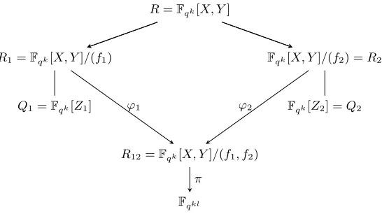
In this section we briefly review the classical FFS and describe some of the recent techniques. The knowledgeable reader may omit this section, having familiarised themself with the notation via a brief look at Fig. 1.
Given the embedding ofFpnintoFqkl as described in the introduction, we focus purely on the latter. A relation in Fqkl is an equality of products of elements inF×
qkl, or, equivalently, a linear combination of logarithms of elements in F×qkl whose sum is zero. All variants of the FFS rely on the following basic method for obtaining relations. Let R =Fqk[X, Y] and let f1, f2 ∈R be two irreducible polynomials such that R12=R/(f1, f2) is a finite ring surjecting onto the target
field Fqkl. Furthermore, for i= 1,2, letRi =Fqk[X, Y]/(fi) and Zi ∈R such that the quotient field Quot(Ri) is a finite extension of the rational function field Quot(Qi) where Qi =Fqk[Zi]. This is summarised in Fig. 1.
R=Fqk[X, Y]
R1=Fqk[X, Y]/(f1) Fqk[X, Y]/(f2) =R2
Q1=Fqk[Z1] F
qk[Z2] =Q2
R12=Fqk[X, Y]/(f1, f2)
Fqkl
ϕ1 ϕ2
π
Fig. 1: Setup for the FFS
Via the maps π, ϕ1 and ϕ2, logarithms in F×qkl can be extended to a notion of logarithms in Ri\(π◦ϕi)−1(0), i= 1,2. Therefore, relations can also be viewed as linear combinations of
logarithms of elements in R1 and in R2 whose sum is zero. It is always implicitly assumed that
all logarithms are defined, i.e., that the sets (π◦ϕi)−1(0), i= 1,2, are avoided.
A polynomial P ∈ R gives rise to a relation by decomposing P modfi in Ri for i = 1,2
elements of a set of bounded size allow one to compute logarithms in this set. If the multiplicative closure of such a set is F×qkl, arbitrary logarithms can be computed by expressing an element as a product of elements of this set. As was described in Section 1, this is done by following a descent strategy in which elements, also called special-Q, are recursively rewritten as ‘easier’ elements using relations as above.
In the classical FFS the polynomials f1, f2 are chosen such that their degrees are as low
as possible, typically of the form f1 = Y −a(X), f2 = Pj=0d bj(X)Yj with degX(a) = e,
degX(bj)< eandde > l, andZ1 =Z2 =X so that the extensions Quot(Ri)/Quot(Qi),i= 1,2,
are of degree 1 and degreed, respectively. By choosingP as a low-degree polynomial, the degrees of the norms NQuot(Ri)/Quot(Qi)(P modfi), i= 1,2, are not too big and therefore the chance of both norms splitting into low-degree polynomials is sufficiently high. With judiciously selected parameters this gives a heuristic running time of L(1/3).
The main difference between the classical FFS and the recent variations [21, 31, 5] is where the relation generation begins. In the recent variations a product of low-degree polynomials
˜
P =QP˜j inR1 is constructed in such a way that it can be lifted to a low-degree polynomial
P ∈Rand such that its reductionP modf2 is of sufficiently low degree, where by low degree we
mean that the norm has low degree. This can be achieved by choosing q to be of the order ofl,
f1 =Y −Xq† and f2 of low degree. Then R1 =Fqk[X] and low-degree polynomials F, G∈R1 give rise to relations via
˜
P =FqG−F Gq=G Y
α∈Fq
(F −αG) =YP˜j, (4)
sinceFq(resp.Gq) can be expressed as a degree degF (resp. degG) polynomial inY, and thus ˜P
can be lifted to a low-degree polynomial P. This yields a heuristic polynomial time algorithm for finding relations between elements ofFqkl that are, via π,ϕ1 andϕ2, images of polynomials of bounded degree.
In the descent phase it is advantageous to choose f2 such that its degree in X or in Y is
one (cf. [25] and [31] respectively), which implies that Quot(R2) = Quot(Q2) with Z2 = Y or
Z2 = X, respectively. More precisely, writing f2 = h1X−h0 or f2 = h1Y −h0 respectively,
with hi ∈Q2,i= 0,1, implies R2 =Fqk[Z2][h11]. Up to the logarithm of h1, the logarithm of a
polynomial ofR1 can be related to the logarithm of a corresponding polynomial inR2(the same
polynomial forZ2 =X and a Frobenius twist forZ2=Y) which allows one to view a special-Q
(the element to be eliminated) as coming from R1 or from R2. In the latter case, the condition
that a polynomial Q ∈ R2, a lift of the special-Q element, divides P modf2 for a P arising
via (4), can be expressed as a bilinear quadratic system which gives, for appropriate parameter choices, an algorithm with heuristic running time L(1/4 +o(1)).
In the other case, namely the special-Q element being lifted to Q ∈ R1, a certain set of
polynomials in R1 containing Qis chosen in such a way that pairs F, G from this set generate
via (4) sufficiently many relations with P modf2 splitting into polynomials of sufficiently low
degree. Solving a linear system of equations then expresses the logarithm of the special-Qelement as a linear combination of logarithms of polynomials in R2 of sufficiently low degree (and h1),
resulting in the original QPA.
Actually, the relations in the original QPA (and in [31]) are generated in a slightly differ-ent manner by applying linear fractional transformations to the polynomial A = Xq−X =
† An interesting historical aside is that this specialisation was also proposed by Shinoharaet alin January 2012
Q
α∈Fq(X−α). The subgroup PGL2(Fq)⊂PGL2(Fqk) is the largest subgroup fixing this poly-nomial, so that the action of PGL2(Fqk)/PGL2(Fq) on A produces q
3k−qk
q3−q polynomials, each splitting into linear polynomials and whose only non-zero terms correspond to the monomials
Xq+1,Xq,X and 1.
4 The descent
In this section we detail the building block behind our new descent and explain why its successful application implies Theorem 2. In the terminology of the previous section, the setup forFqkl has
f1 =Y−Xqandf2=h1Y−h0withhi ∈Fqk[X] of degree at most two fori= 0,1, withh1Xq−h0
having an irreducible factor I of degreel, i.e., R12=Fqk[X, Y]/(f1, f2) surjects ontoFqkl.† This impliesR1 =Fqk[X] andR2=Fqk[X][h1
1]. We assume (without loss of generality) thath0 andh1 are coprime. By the phrase “rewriting a polynomial Q(inR1 orR2) in terms of polynomialsPi
(in R1 or R2)” we henceforth mean that in the target field the image of Q equals a product
of powers of images of Pi. Since h1 appears in almost every relation, we adjoin it to the factor
basisF, and for the sake of simplicity it is suppressed in the following description.
4.1 On-the-fly degree two elimination
In this subsection we review the on-the-fly degree two elimination method from [21], adjusted for the present framework. In [6] the affine portion of the set of polynomials obtained as linear fractional transformations of Xq−X is parameterised as follows. Let B be the set of B ∈Fqk such that the polynomial Xq+1−BX+B splits completely overF
qk, the cardinality of which is approximately qk−3 [6, Lemma 4.4]. Scaling and translating these polynomials means that all
the polynomials Xq+1+aXq+bX+c with c6=ab,b6=aq and B = (b(c−−aqab))q+1q split completely overFqk wheneverB ∈ B.
LetQ(viewed as a polynomial inR2) be an irreducible quadratic polynomial to be eliminated.
We let LQ ⊂Fqk[X]2 be the lattice defined by
LQ ={(w0, w1)∈Fqk[X]2 |w0h0+w1h1≡0 (mod Q)}. (5)
In the case that Qdivides w0h0+w1h1 6= 0 for some w0, w1 ∈ Fqk, then Q =w(w0h0+w1h1) for somew∈F×qk, since the degree on the right hand side is at most two. Therefore, the relation generated fromP =w0Y +w1∈RrelatesQwithw0Xq+w1 = (w01/qX+w11/q)q∈R1 (andh1).
We will say in this case that the lattice is degenerate.
In the other (non-degenerate) case,LQ has a basis of the form (1, u0X+u1),(X, v0X+v1)
withui, vi∈Fqk. Since the polynomialP =XY+aY+bX+cmaps to h1
1((X+a)h0+(bX+c)h1) in R2, Q divides P modf2 if and only if (X +a, bX +c) ∈ LQ. Note that the numerator of
P modf2 is of degree at most three, thus it can at worst contain a linear factor besides Q. If
the triple (a, b, c) also satisfiesc6=ab,b6=aq and (b(c−−aqab))q+1q ∈ B, thenP modf1 splits into linear
factors and thusQ has been rewritten in terms of linear polynomials.
Algorithmically, a triple (a, b, c) satisfying all conditions can be found in several ways. Choos-ing aB∈ B, considering (X+a, bX+c) =a(1, u0X+u1)+(X, v0X+v1) and rewritingb=u0a+v0
and c=u1a+v1 gives the condition
B = (−a
q+u
0a+v0)q+1
(−u0a2+ (−v0+u1)a+v1)q
. (6)
By expressing a in anFqk/Fq basis, (6) results in a quadratic system ink variables [22]. Using a Gr¨obner basis algorithm the running time is exponential in k. Alternatively, and this is one
† One can equally well work withf
of the key observations for the present work, equation (6) can be considered as a polynomial of degree q2+q in a whose roots can be found in polynomial time in q and in k by taking a GCD with aqk
−a in Fqk[a] [21]. One can also check for random (a, b, c) such that the lattice condition holds, whether Xq+1+aXq+bX+c splits into linear polynomials, which happens with probability q−3. Each such instance is also polynomial time in q and in k.
These degree 2 elimination methods will fail whenQdividesh1Xq−h0, because this would
imply that the polynomialP modf1 =Xq+1+aXq+bX+cis divisible byQwheneverP modf2
is, a problem first discussed in [8]. Such polynomialsQor their roots will be called traps of level 0. Similarly, these degree 2 elimination methods might also fail when Q dividesh1Xq
k+1
−h0, in
which case such polynomials Qor their roots will be called traps of levelk.
Note that for Kummer extensions, i.e., whenh1= 1 andh0 =aX for somea∈Fqk, there are no traps and hence much of the following treatment is not required for proving only Theorem 1. However, it is essential to consider traps for proving the far more general Theorem 2.
4.2 Elimination requirements
As briefly explained in the introduction, the on-the-fly degree two elimination method can be transformed into an elimination method for irreducible even degree polynomials. We now present a theorem which states that under some assumptions this degree two elimination is guaranteed to succeed, and subsequently demonstrate that it implies Theorem 2.
An element τ ∈ Fqk for which [Fqk(τ) : Fqk] = 2d is even and h1(τ) 6= 0, is called a trap root if it is a root of h1Xq−h0 orh1Xq
kd+1
−h0, or if hh01(τ)∈Fqkd. Note that the sets of trap roots is invariant under the absolute Galois group of Fqk. A polynomial in R1 orR2 is said to be good if it has no trap roots; the same definitions are used when the base field of R1 and R2
is extended. This definition encompasses traps of level 0, of level kd, and the case where for
Q6=h1 the latticeLQ is degenerate.
Theorem 3. Let q > 61 be a prime power that is not a power of 4, let k ≥ 18 be an integer and let h0, h1 ∈Fqk[X] be of degree at most two with h1Xq−h0 having an irreducible degree l
factor. Moreover, let d≥1 be an integer, let Q ∈Fqkd[X], Q 6=h1 be an irreducible quadratic good polynomial, and let (1, u0X+u1),(X, v0X+v1) be a basis of the lattice LQ in (5). Then
the number of solutions (a, B)∈Fqkd× B of (6) resulting in good descendents is at least qkd−5. This theorem is of central importance for our rigorous analysis and is proven in Section 5.
4.3 Degree 2d elimination and descent complexity
Now we demonstrate how the on-the-fly degree two elimination gives rise to a method for elim-inating irreducible even degree polynomials, which is the crucial building block for our descent algorithm. As per Theorem 3, let q >61 be a prime power that is not a power of 4, let k≥18, and let h0, h1, I as before.
Proposition 1. Let Q∈R2, Q6=h1, be an irreducible good polynomial of degree 2d. Then Q
can be expressed in terms of at most q+ 2 irreducible good polynomials of degrees dividing d, in an expected running time polynomial in q and in d.
Proof. Over the extension Fqkd the polynomial Qsplits into dirreducible good quadratic poly-nomials; let Q′ be one of them. Since Q′ 6=h1 is good it does not divide w0h0 +w1h1 6= 0 for
somew0, w1 ∈Fqkd. By Theorem 3, with an expected polynomial number of trials, the on-the-fly degree two elimination method for Q′ ∈ Fqkd[X] produces a polynomial P′ ∈ Fqkd[X, Y] such that P′modf1 splits into a product of at mostq+ 1 good polynomials of degree one over Fqkd and such that (P′ modf
Let P be the product of all conjugates ofP′ under Gal(Fqkd/Fqk). Since the product of all con-jugates of a linear polynomial under Gal(Fqkd/Fqk) is thed1-th power of an irreducible degreed2 polynomial for d1 and d2 satisfying d1d2 =d, the rewriting assertion of the proposition follows.
The three steps of this method – computingQ′, the on-the-fly degree two elimination (when the second or third approach listed above for solving (6) is used), and the computation of the polynomial norms – all have running time polynomial in q and ind, which proves the running
time assertion. ⊓⊔
By recursively applying Proposition 1 we can express a good irreducible polynomial of degree 2e,e≥1, in terms of at most (q+ 2)elinear polynomials. The final step of this recursion, namely eliminating up to (q+ 2)e−1 quadratic polynomials, dominates the running time, which is thus upper bounded by (q+ 2)e times a polynomial inq.
Lemma 2. Any nonzero element in Fqkl can be lifted to an irreducible good polynomial of de-gree 2e, provided that 2e>4l.
Proof. By the effective Dirichlet-type theorem on irreducibles in arithmetic progressions [53, Thm. 5.1], for 2e > 4l the probability of irreducibility for a random lift is lower bounded by 2−e−1. One may actually find an irreducible polynomial of degree 2e which is good, since the
number of possible trap roots (< qk2e−1+2) is much smaller than the number (> qk(2e−l)2−e−1)
of irreducibles produced by this Dirichlet-type theorem. ⊓⊔
Putting everything together, this proves the quasi-polynomial expected running time of the descent and therefore the running time of our algorithm in Section 2, establishing Theorem 2.
Note that forq =Lqkl(α), just as in [5], the complexity stated in Theorem 2 is L(α+o(1)), which is therefore better than the classical FFS for α < 13.
Finally note that during an elimination step, one need not use the basic building block as stated, which takes the norms of the linear polynomials produced back down to Fqk. Instead, one need only take their norms to a subfield of index 2, thus becoming quadratic polynomials, and then recurse, as depicted in Fig. 2.
1 2 2e
F
qknF
q2kn 1 2F
q4kn 1 2.. . .. .
F
q2e−2kn 1 2F
q2e−1kn 1 2Fig. 2: Elimination of irreducible polynomials of degree a power of 2 when considered as elements ofFqk[X]. The
5 Proof of Theorem 3
In this section we prove Theorem 3, which by the arguments of the previous section demonstrates the correctness of our algorithm and our main theorems.
5.1 Notation and statement of supporting results
LetK =Fqkd withkd≥18, letL=Fq2kd be its quadratic extension, and letQbe an irreducible quadratic polynomial inK[X] such that (1, u0X+u1),(X, v0X+v1) is a basis of its associated
latticeLQ in (5). ThenQ is a scalar multiple of−u0X2+ (−u1+v0)X+v1.
Let B be the set of B ∈ K such that the polynomial Xq+1−BX+B splits completely overK. Using an elementary extension of [29, Theorem 5] the setBcan be characterised as the image of K\Fq2 under the map
u7→ (u−u
q2 )q+1
(u−uq)q2+1. (7)
By this and (6), in order to eliminateQ we need to find (a, u)∈K×(K\Fq2) satisfying
(u−uq2)q+1(−u0a2+ (−v0+u1)a+v1)q−(u−uq)q
2+1
(−aq+u0a+v0)q+1 = 0.
The two terms have a common factor (u−uq)q+1 which motivates the following definitions. Let
α=−u0,β =u1−v0,γ =v1 and δ=−v0 withα, β, γ, δ∈K, as well as
D= U
q2 −U Uq−U =
Y
ǫ∈Fq2\Fq
(U −ǫ),
E=Uq−U = Y
ǫ∈Fq
(U−ǫ),
F =αA2+βA+γ =α(A−ρ1)(A−ρ2) with ρ1, ρ2 ∈L,
G=Aq+αA+δ and
P =Dq+1Fq−Eq2−qGq+1∈K[A, U].
Note thatF equalsQ(−A) (up to a scalar), so that deg(F) = 2,F is irreducible and ρ1, ρ2 ∈/ K.
We consider the curve C defined by P = 0 and are interested in the number of (affine) points (a, u)∈C(K) withu /∈Fq2. More precisely, we want to prove the following.
Theorem 4. Let q >61 be a prime power that is not a power of 4. If the conditions
(∗) ρq1+αρ2+δ6= 0
(∗∗) ρq1+αρ1+δ6= 0
hold then there are at least qkd−1 pairs (a, u)∈K×(K\Fq2) satisfying P(a, u) = 0.
The relation of the two conditions to the quadratic polynomial Q as well as properties of traps are described in the following propositions.
Proposition 2. If condition (∗) is not satisfied, then Q divides h1Xq−h0, i.e., Q is a trap
of level 0. If condition (∗∗) is not satisfied, then Q divides h1Xq
kd+1
−h0, i.e., Q is a trap of
level kd. In particular, if Qis a good polynomial then conditions (∗) and (∗∗) are satisfied.
Proposition 3. Let (a, u),(a′, u′) ∈ K ×(K \F
q2) be two solutions of P = 0 with a 6= a′, corresponding to the polynomials Pa = XY +aY +bX+c and Pa′ = XY +a′Y +b′X+c′,
respectively. ThenPamodf1 andPa′ modf1 have no common roots. Furthermore, the common
Now we explain how (forq >61 not a power of 4) Theorem 3 follows from the above theorem and the propositions. Since the irreducible quadratic polynomial Q is good, the lattice LQ is
non-degenerate so that a basis as above exists, and by Proposition 2 the two conditions of Theorem 4 are satisfied. The map (7) is q3−q : 1 on K \Fq2, hence there are at least qkd−4 solutions (a, B) ∈ K × B of (6), which contain at least qkd−4 different values a∈ K. Observe that a trap rootτ that may occur in this situation is a root ofh1Xq−h0, or ofh1Xq
kd′+1 −h0
for d′ | d2, or it satisfies h0
h1(τ) ∈ Fqkd/2. The cardinalities of these trap roots is at most q kd
2+3. By Proposition 3 a trap root can appear in Pamodfj for at most two values a, at most once
forj= 1 and at most once for j= 2. Hence there are at mostqkd2+4 < qkd−5 valuesafor which a trap root appears in Pamodfj,j = 1,2. Thus there are at least qkd−5 different values a for
which a solution (a, B) leads to an elimination into good polynomials. This finishes the proof of Theorem 3, hence we focus on proving the theorem and the two propositions above.
5.2 Outline of the proof method
The main step of the proof of the theorem consists in showing that, subject to conditions (∗) and (∗∗), there exists an absolutely irreducible factorP1 ofP that lies already inK[A, U]. Since
the (total) degree of P1 is at most q3+q, restricting to the component of the curve defined
by P1 and using the Weil bound for possibly singular plane curves gives a lower bound on the
cardinality of C(K) which is large enough to prove the theorem after accounting for projective points and points with second coordinate in Fq2. This argument is given in the next subsection before dealing with the more involved main step.
For proving the main step the action of PGL2(Fq) on the variable U is considered. An
ab-solutely irreducible factor P1 of P is stabilised by a subgroup S1 ⊂PGL2(Fq) satisfying some
conditions. The first step is to show that, after possibly switching to another absolutely irre-ducible factor, there are only a few cases for the subgroup. Then for each case it is shown that the factor is defined overK[A, U] or that one of the conditions on the parameters is not satisfied.
The propositions are proven in the final subsection.
5.3 Weil bound
LetC1be the absolutely irreducible plane curve defined byP1of degreed1≤q3+q2. Corollary 2.5
of [4] shows that
|#C1(K)−qkd−1| ≤(d1−1)(d1−2)q
kd 2 .
Since degA(P1) ≤ q2+q there are at most q4+q3 affine points with u ∈ Fq2. The number of points at infinity is at most d1 ≤ q3+q2 < q4. Denoting by C1(K)ethe set of affine points in
C1(K) with second coordinateu6∈Fq2 one obtains
|#C1(K)e|> qkd−(q4+q3)−d1−(d1−1)(d1−2)q
kd
2 > qkd−q kd
2+8 ≥qkd−1,
sincekd≥18, thus proving the theorem if there exists an absolutely irreducible factorP1 defined
overK[A, U].
5.4 PGL2 action
Here the following convention for the action of PGL2(Fq) on P1 and on polynomials is used.
A matrix
a b c d
∈ PGL2(Fq) acts on P1(M), where M is an arbitrary field containing Fq, by
(x0 :x1)7→
a b c d
(x0 :x1) = (ax0+bx1 :cx0+dx1) or, via P1(M) =M∪ {∞}, by x7→ ax+bcx+d.
σ(τ(x)) = (στ)(x). On a homogeneous polynomial H in the variables (X0 :X1) the action of σ = a b c d
is given byHσ(X0 :X1) =H(aX0+bX1:cX0+dX1). This is an action on the right,
satisfying H(στ) = (Hσ)τ. In the following we will usually use this action on the dehomogenised
polynomials given by Hσ(X) =H(aX+bcX+d), clearing denominators in the appropriate way. The polynomialP ∈(K[A])[U] is invariant under PGL2(Fq) acting on the variableU; this can
be checked by considering the actions of 1b 0 1 , a0 0 1 and 0 1 1 0
, and noticing that PGL2(Fq)
is generated by these matrices. Let
P =s
g
Y
i=1
Pi, Pi ∈(K[A])[U], s∈K[A],
be the decomposition of P in (K[A])[U] into irreducible factors Pi and possibly reducible s.
Notice thatsmust divideFqandGq+1, hence it divides a power of gcd(F, G). AsF is irreducible, gcd(F, G) is either constant or of degree two. In the latter case ρ1 is a root of Gcontradicting
condition (∗∗). Therefore one can assume thats∈K is a constant. Let
P =Fq
q3−q Y
i=1
(U−ri), ri ∈K(A),
be the decomposition of P in K(A)[U]. Then PGL2(Fq) permutes the set {ri} and, since fixed
points of PGL2(Fq) lie in Fq2 but ri ∈/ Fq2, the action is free. Since # PGL2(Fq) = q3 −q the action is transitive.
Therefore the action on the decomposition overK[A, U] is also transitive (adjusting the Pi
by scalars inK[A] if necessary). Denoting bySi ⊂PGL2(Fq) the stabiliser ofPiit follows that all
Si are conjugates of each other, thus they have the same cardinality and henceq3−q=g·#Si.
Moreover the degree of Pi in U is constant, namely #Si, and also the degree of Pi in A is
constant, thus g|q2+q= deg
A(P). In particular, q−1|#Si.
5.5 Subgroups of PGL2
The classification of subgroups of PSL2(Fq) is well known [15] and allows to determine all
subgroups of PGL2(Fq) [7]. Since #Si is divisible by q−1 (in particular #Si > 60), only the
following subgroups are of interest (per conjugation class only one subgroup is listed):
1. the cyclic group
∗0 0 1
of order q−1,
2. the dihedral group ∗0 0 1 ∪ 0 1 ∗0
of order 2(q−1) and, ifqis odd, its two dihedral subgroups
na0 0 1
|a6= 0 a squareo∪n0 1
c0
|c6= 0 a squareo and
na0 0 1
|a6= 0 a squareo∪n0 1
c0
|cnot a squareo,
both of orderq−1,
3. the Borel subgroup
∗ ∗ 0 1
of order q2−q,
4. if q is odd, PSL2(Fq) of index 2,
5. if q=q′2 is a square, PGL2(Fq′) of orderq′3−q′=q′(q−1), and
In the last caseP is absolutely irreducible, thus it remains to investigate the first five cases which are treated in the next subsection.
Remark: The conditionq >61 rules out some small subgroups asA4, S4, andA5. In many
of the finitely many cases q ≤61 the proof of the theorem also works (e.g., q not a square and
q−1∤120). The condition ofq not being a power of even exponent of 2 eliminates the fifth case in characteristic 2; removing this condition would be of some interest.
5.6 The individual cases
Since the stabilisers Si are conjugates of each other, one can assume without loss of generality
that S1 is one of the explicit subgroups given in the previous subsection. Then the polynomial
P1 is invariant under certain transformations of U, so that P1 and P can be rewritten in terms
of another variable as stated in the following.
If a polynomial (in the variableU) is invariant underU 7→aU,a∈F×q, it can be considered as a polynomial in the variableV =Uq−1. For the polynomials Dand Eq−1 one obtains
D= V
q+1−1
V −1 and E
q−1 =V(V −1)q−1.
Similarly, in the case of odd q, if a polynomial is invariant under U 7→ aU for all squares
a∈F×
q, it can be rewritten in the variableV′ =U
q−1
2 . ForD and Eq−1 this gives
D= V
′2q+2−1
V′2−1 and E
q−1 =V′2(V′2−1)q−1.
If a polynomial is invariant underU 7→U +b,b∈Fq, it can be considered as a polynomial in ˜V =Uq−U which gives
D= ˜Vq−1+ 1 and Eq−1 = ˜Vq−1.
Combining the above yields that a polynomial which is invariant under both U 7→ aU,
a∈F×q, andU 7→U+b,b∈Fq, can be considered as a polynomial inW = ˜Vq−1 = (Uq−U)q−1.
For Dand Eq−1 one obtains
D=W + 1 and Eq−1=W.
This is now applied to the various cases forS1.
The cyclic case Rewriting P and P1 in terms ofV =Uq−1 one obtains
P =V
q+1−1
V −1 q+1
Fq−Vq(V −1)q2−qGq+1
and degV(P1) = 1, i.e.,P1 =p1V−p0 withpi∈K[A], gcd(p0, p1) = 1, max(deg(p0),deg(p1)) = 1
and it can be assumed that p0 is monic.
The divisibilityP1 |P transforms into the following polynomial identity in K[A]:
pq+1 0 −p
q+1 1
p0−p1
q+1
Fq =pq1p0q(p0−p1)q
2
−qGq+1.
The degree of the first factor on the left hand side is either q2 +q or q2 −1 (if p0 −ζp1 is
constant for some ζ ∈ µq+1(Fq2)\ {1}). Since the degrees of the other factors are all divisible by q, the latter case is impossible. Since deg(F) = 2 one gets deg(Fq) = 2q. Furthermore, deg((p0p1)q) ∈ {q,2q}, deg((p0−p1)q
2−q
Letp0−p1 =c1 ∈K; in the following ci will be some constants inK. Since the first factor
on the left hand side is coprime to p0p1, it follows
pq+10 −pq+11 p0−p1
=c2G, F =c3p0p1 and cq+12 c q 3 =c
q2−q
1 .
Exchanging ρ1 and ρ2, if needed, one obtains
p0 =A−ρ1, p1 =A−ρ2, c3=α and c1 =ρ2−ρ1.
Considering the coefficient ofAqin the equation forGgivesc
2= 1 and evaluating this equation
atA=ρ2 gives
ρq1+αρ2+δ= 0.
This means that condition (∗) does not hold.
The dihedral cases The case of the dihedral group of order 2(q−1) is considered first. Then, as above,P andP1 can be expressed in terms ofV, and, sinceP andP1 are also invariant under
V 7→ V1, they can be expressed in terms of W+ = V +V1. This gives degW+(P1) = 1 and with Z =µq+1(Fq2)\ {1}
Dq+1V−q
2+q
2 =
Y
ζ∈Z
(W+−(ζ+ζq))
q+1
2 and
P V−q
2+q
2 =
Y
ζ∈Z
(W+−(ζ+ζq))
q+1 2
Fq−(W+−2)
q2−q 2 Gq+1.
In characteristic 2 each factor of the product over Z appears twice, thus justifying their expo-nent q+12 .
By writing P1 = p1W+−p0, with pi ∈ K[A], gcd(p0, p1) = 1, max(deg(p0),deg(p1)) = 2
and p0 being monic, the divisibility P1 | P transforms into the following polynomial identity
inK[A]:
Y
ζ∈Z
(p0−(ζ+ζq)p1)
q+1 2
Fq=pq1(p0−2p1)
q2−q 2 Gq+1.
Again the degree of the first factor on the left hand side must be divisible by q (respectively,
q
2 in characteristic 2), and since p0−(ζ+ζq)p1 can be constant or linear for at most one sum
ζ+ζq, the degree of the first factor must beq2+q forq >4. Also the degree ofp0−2p1 must
be zero since q >3 and thus the degree ofp1 is 2.
In even characteristicp0−2p1=p0 is a constant, thusp0 = 1 (p0 is monic). The involution
ζ 7→ζq =ζ−1 onZhas no fixed points, and, denoting byZ
2a set of representatives ofZmodulo
the involution, one obtains Y
ζ∈Z2
(1−(ζ+ζq)p1) =c1G, F =c2p1 and cq+11 c q 2= 1.
Modulo F one gets F |c1G−1 which implies c1 ∈K. Thus c2 ∈K, p1 ∈K[A] and therefore
P1∈K[A, U].
In odd characteristic the factor corresponding to ζ =−1, namely (p0+ 2p1)
q+1
2 , is coprime to the other factors in the product and coprime top1(p0−2p1). Hencep0+ 2p1must be a square
and its square root must divideG. Moreover, one getsF =c1p1. Sincep0−2p1=c2is a constant
and p0 is monic, one getsc1 = 2α, implyingp1 ∈K[A]. Sincep0+ 2p1 = 4p1+c2 is a square, its
IfS1 is one of the two dihedral subgroups of order q−1 (which implies that q is odd), the
argumentation is similar. The polynomials P and P1 are expressed in terms of V′ =U
q−1 2 and then, since U 7→ cU1 becomes V′ 7→ c−q−1
2 1
V′ with c−
q−1
2 = ±1, in terms of W′
+ = V′ + V1′ or
W−′ =V′−V1′, respectively. In the first case P is rewritten as
P V′−(q2+q)= Y
ζ∈Z′
(W+′ −(ζ+ζ−1))q+12
Fq−(W+′ −2)q 2
−q 2 (W′
++ 2)
q2−q 2 Gq+1
where Z′ =µ
2(q+1)(Fq2)\ {±1}. By setting P1 = p1W+′ −p0 with pi ∈ K[A], gcd(p0, p1) = 1, max(deg(p0),deg(p1)) = 1 andp0 being monic, one obtains
Y
ζ∈Z′
(p0−(ζ+ζ−1)p1)
q+1 2
Fq =p2q1 (p0−2p1)
q2−q
2 (p0+ 2p1) q2−q
2 Gq+1.
Since one ofp0±2p1 is not constant, the degree of the right hand side exceeds the degree of the
left hand side for q >5 which is a contradiction. In the second caseP is rewritten as
P V′−(q2+q)= Y
ζ∈Z′
(W−′ −(ζ−ζ−1))q+12
Fq−W−′q2−qGq+1
and by setting P1 =p1W−′ −p0 with pi∈K[A], gcd(p0, p1) = 1, max(deg(p0),deg(p1)) = 1 and
p0 being monic, one obtains
Y
ζ∈Z′
(p0−(ζ−ζ−1)p1)
q+1 2
Fq =p2q1 pq02−qGq+1.
Considering the degrees for q >3 it follows thatp0 must be constant and hence p1 is of degree
one. Sincep1 is coprime to the first factor on the left hand side, it must divideFq which implies
ρ1=ρ2 ∈K, contradicting the irreducibility of F.
The Borel case In this case, rewriting P and P1 in terms ofW = (Uq−U)q−1 gives
P = (W + 1)q+1Fq−WqGq+1
and degW(P1) = 1, P1 =p1W −p0, withpi∈K[A], gcd(p0, p1) = 1, max(deg(p0),deg(p1)) =q
andp1being monic. Then the divisibilityP1 |Ptransforms into the following polynomial identity
inK[A]:
(p0+p1)q+1Fq =p1pq0Gq+1.
From deg(Gq+1) =q2+q, deg(p
1pq0)≥q and deg(Fq) = 2q it follows that the degree ofp0+p1
must be q. This implies deg(Fq) = deg(p1pq0), thus deg(p0)≤2 and therefore deg(p1) =q, since
q >2, and deg(p0) = 1.
Sincep0+p1 is coprime top0p1, it follows
p0+p1=c1G, p1 = ˜pq, F =c2pp˜ 0 and cq+11 c q 2= 1
for a monic linear polynomial ˜p∈K[A].
Exchangingρ1 and ρ2, if needed, one obtains
˜
p=A−ρ1, p0=c3(A−ρ2), c1 = 1, c2= 1 and c3 =α.
Evaluating p0+p1 =G atA= 0 gives
ρq1+αρ2+δ= 0.
The PSL2 case This case can only occur for odd q, and then P splits as P =sP1P2 with a
scalar s∈K. The map U 7→ aU for a non-squarea∈Fq exchanges P1 and P2. Since PSL2(Fq)
is a normal subgroup of PGL2(Fq), P2 is invariant under PSL2(Fq) as well. By rewriting P in
terms of W′ = (Uq−U)q−21 one obtains
P = (W′2+ 1)q+1Fq−W′2qGq+1 =sP1(W′)P1(−W′).
Denoting by p0 ∈K[A] the constant coefficient ofP1∈(K[A])[W′] this becomes modulo W′
Fq=sp20
which implies ρ1 =ρ2∈K, contradicting the irreducibility ofF.
The case PGL2(Fq′) Since PGL2(Fq′)⊂PSL2(Fq) in odd characteristic, one can reduce this
case to the previous case as follows.
Let I1 ⊂ {1, . . . , g} be the subset of i such that Si is a conjugate of S1 by an element in
PSL2(Fq), and letI2 ={1, . . . , g} \I1. These two sets correspond to the two orbits of the action
of PSL2(Fq) on theSi (orPi). Both orbits contain #I1 = #I2 = g2 elements and an element in
PGL2(Fq)\PSL2(Fq) transfers one orbit into the other.
Let ˜Pj =Qi∈IjPi,j = 1,2, then P splits as P =sP˜1P˜2,s∈K, and both ˜Pj, j = 1,2, are invariant under PSL2(Fq). Notice that the absolute irreducibility ofP1 and P2 was not used in
the argument in the PSL2 case.
This completes the proof of Theorem 4.
5.7 Traps
In the following Proposition 2 and Proposition 3 are proven.
LetQbe an irreducible quadratic polynomial inK[X] such that (1, u0X+u1),(X, v0X+v1)
is a basis of the latticeLQ, so thatQis a scalar multiple of−u0X2+ (−u1+v0)X+v1=F(−X)
and has roots −ρ1 and −ρ2. By definition of LQ the pair (h0, h1) must be in the dual lattice
(scaled by Q), given by the basis (u0X+u1,−1),(v0X+v1,−X).
For the assertions concerning conditions (∗) and (∗∗), assume that ρ1, ρ2∈L\K and that
ρq1+αρj +δ = 0
holds for j= 1 or j = 2.
First consider the case j = 2, i.e., condition (∗). To show that −ρi, i = 1,2, are roots of
h1Xq−h0 it is sufficient to show this for the basis of the dual lattice of LQ given above. For
(u0X+u1,−1) one computes
−(−ρq1)−u0(−ρ1)−u1=ρ1q−αρ1−β+δ =−αρ2−αρ1−β = 0,
and for (v0X+v1,−X) one obtains
−(−ρ1)(−ρq1)−v0(−ρ1)−v1= (−ρq1−δ)ρ1−γ =αρ1ρ2−γ = 0.
Thereforeh1Xq−h0 is divisible byQ, which is then a trap of level 0.
In the casej= 1 an analogous calculation shows that−ρi,i= 1,2, are roots ofh1Xq
kd+1 −h0,
namely for (u0X+u1,−1) one has
−(−ρq2kd+1)−u0(−ρ2)−u1 =ρq1−αρ2−β+δ=−αρ1−αρ2−β = 0
and for (v0X+v1,−X) one gets
−(−ρ2)(−ρq
kd+1
Therefore h1Xq
kd+1
−h0 is divisible by Q, which is then a trap of level kd. This finishes the
proof of Proposition 2.
Regarding Proposition 3, note that a solution (a, B) gives rise to the polynomial Pa =
a(u0X+ (Y +u1)) + ((Y +v0)X+v1). If, for j = 1 or j = 2, ρ is a root of Pamodfj for two
different values of a, thenρ is a root of u0X+ (Y +u1) modfj and of (Y +v0)X+v1 modfj.
Since
−X(u0X+ (Y +u1)) + (Y +v0)X+v1 =−u0X2+ (−u1+v0)X+v1 =F(−X),
which equalsQup to a scalar, it follows thatρis also a root ofQ. Furthermore, in the casej= 1 the polynomial Pamodf1 splits completely, so that ρ ∈ K, contradicting the irreducibility of
Q, finishing the proof of Proposition 3. This completes the proof of Theorem 3.
Acknowledgements
The authors are indebted to Claus Diem for explaining how one can obviate the need to compute the logarithms of the factor base elements, and wish to thank him also for some enlightening discussions.
References
1. Leonard M. Adleman. A subexponential algorithm for the discrete logarithm problem with applications to cryptography. InProceedings of the 20th Annual Symposium on Foundations of Computer Science, SFCS ’79, pages 55–60, Washington, DC, USA, 1979. IEEE Computer Society.
2. Leonard M. Adleman. The function field sieve. In Leonard M. Adleman and Ming-Deh Huang, editors,
Algorithmic Number Theory, volume 877 ofLecture Notes in Computer Science, pages 108–121. Springer Berlin Heidelberg, 1994.
3. Leonard M. Adleman and Ming-Deh A. Huang. Function field sieve method for discrete logarithms over finite fields. Inform. and Comput., 151(1-2):5–16, 1999.
4. Yves Aubry and Marc Perret. A Weil theorem for singular curves. InArithmetic, geometry and coding theory (Luminy, 1993), pages 1–7. de Gruyter, Berlin, 1996.
5. Razvan Barbulescu, Pierrick Gaudry, Antoine Joux, and Emmanuel Thom´e. A heuristic quasi-polynomial algorithm for discrete logarithm in finite fields of small characteristic. In Advances in Cryptology— EUROCRYPT 2014, volume 8441 ofLNCS, pages 1–16. Springer, 2014.
6. Antonia W. Bluher. Onxq+1+ax+b. Finite Fields and Their Applications, 10(3):285–305, 2004.
7. Peter J. Cameron, Gholam R. Omidi, and Behruz Tayfeh-Rezaie. 3-designs from PGL(2, q). Electron. J. Combin., 13(1):Research Paper 50, 11, 2006.
8. Qi Cheng, Daqing Wan, and Jincheng Zhuang. Traps to the bgjt-algorithm for discrete logarithms. LMS Journal of Computation and Mathematics, 17:218–229, 2014.
9. Fan-Rong K. Chung. Diameters and eigenvalues. J. Amer. Math. Soc., 2(2):187–196, 1989.
10. Don Coppersmith. Evaluating logarithms in GF(2n). InProceedings of the Sixteenth Annual ACM Symposium on Theory of Computing, STOC ’84, pages 201–207, New York, NY, USA, 1984. ACM.
11. Don Coppersmith. Fast evaluation of logarithms in fields of characteristic two. IEEE Trans. Inf. Theor., 30(4):587–594, 1984.
12. Nicolaas G. De Bruijn. On the number of positive integers≤xand free of prime factors> y. Indagationes Mathematicae, 13:50–60, 1951.
13. Nicolaas G. De Bruijn. On the number of positive integers≤xand free of prime factors> y, II.Indagationes Mathematicae, 28:239–247, 1966.
14. Karl Dickman. On the frequency of numbers containing prime factors of a certain relative magnitude. Arkiv f¨or Matematik, Astonomi och Fysik, 22A (10):1–14, 1930.
15. Leonard E. Dickson. Linear groups: With an exposition of the Galois field theory. Teubner, Leipzig, 1901. 16. Claus Diem. On the discrete logarithm problem in elliptic curves. Compositio Mathematica, 147:75–104, 1
2011.
17. Whitfield Diffie and Martin E. Hellman. New directions in cryptography.IEEE Trans. Inf. Theor., 22(6):644– 654, September 2006.
18. Andreas Enge and Pierrick Gaudry. A general framework for subexponential discrete logarithm algorithms.
Acta Arithmetica, 102:83–103, 2002.
20. Faruk G¨olo˘glu, Robert Granger, Gary McGuire, and Jens Zumbr¨agel. On the function field sieve and the impact of higher splitting probabilities. Available fromeprint.iacr.org/2013/074, 15th Feb 2013.
21. Faruk G¨olo˘glu, Robert Granger, Gary McGuire, and Jens Zumbr¨agel. On the function field sieve and the impact of higher splitting probabilities. In Ran Canetti and Juan A. Garay, editors,Advances in Cryptology— CRYPTO 2013, volume 8043 ofLNCS, pages 109–128. Springer, 2013.
22. Faruk G¨olo˘glu, Robert Granger, Gary McGuire, and Jens Zumbr¨agel. Solving a 6120-bit DLP on a desktop computer. InSelected Areas in Cryptography—SAC 2013, volume 8282 ofLNCS, pages 136–152. Springer, 2014.
23. Faruk G¨olo˘glu, Robert Granger, Gary McGuire, and Jens Zumbr¨agel. Discrete Logarithms in GF(21971 ). NMBRTHRY list, 19/2/2013.
24. Faruk G¨olo˘glu, Robert Granger, Gary McGuire, and Jens Zumbr¨agel. Discrete Logarithms in GF(26120 ). NMBRTHRY list, 11/4/2013.
25. Robert Granger, Thorsten Kleinjung, and Jens Zumbr¨agel. Breaking ’128-bit secure’ supersingular binary curves - (or how to solve discrete logarithms inF24·1223 andF212·367). InAdvances in Cryptology—CRYPTO
2014, volume 8617 ofLNCS, pages 126–145. Springer, 2014.
26. Robert Granger, Thorsten Kleinjung, and Jens Zumbr¨agel. On the powers of 2. Available fromeprint.iacr. org/2014/300, 29th Apr 2014.
27. Robert Granger, Thorsten Kleinjung, and Jens Zumbr¨agel. Discrete logarithms in the Jacobian of a genus 2 supersingular curve overGF(2367). NMBRTHRY list, 30/1/2014.
28. Robert Granger, Thorsten Kleinjung, and Jens Zumbr¨agel. Discrete Logarithms inGF(29234
). NMBRTHRY list, 31/1/2014.
29. Tor Helleseth and Alexander Kholosha. x2l+1+x+aand related affine polynomials over GF(2k). Cryptogr.
Commun., 2(1):85–109, 2010.
30. Antoine Joux. Faster index calculus for the medium prime case. application to 1175-bit and 1425-bit finite fields. In Thomas Johansson and Phong Q. Nguyen, editors,Advances in Cryptology—EUROCRYPT 2013, volume 7881 ofLNCS, pages 177–193. Springer, 2013.
31. Antoine Joux. A new index calculus algorithm with complexityL(1/4 +o(1)) in small characteristic. In Tanja Lange, Kristin Lauter, and Petr Lison˘ek, editors, Selected Areas in Cryptography—SAC 2013, volume 8282 ofLNCS, pages 355–379. Springer, 2014.
32. Antoine Joux. A new index calculus algorithm with complexity L(1/4 +o(1)) in very small characteristic. Available fromeprint.iacr.org/2013/095, 20th Feb 2013.
33. Antoine Joux. Discrete Logarithms inGF(21778
). NMBRTHRY list, 11/2/2013. 34. Antoine Joux. Discrete Logarithms inGF(24080
). NMBRTHRY list, 22/3/2013. 35. Antoine Joux. Discrete Logarithms inGF(26168). NMBRTHRY list, 21/5/2013.
36. Antoine Joux and Reynald Lercier. The function field sieve is quite special. In Claus Fieker and David R. Kohel, editors,Algorithmic number theory (Sydney, 2002), volume 2369 ofLNCS, pages 431–445. Springer, 2002.
37. Antoine Joux and Reynald Lercier. The function field sieve in the medium prime case. In Serge Vaudenay, editor,Advances in Cryptology—EUROCRYPT 2006, volume 4004 ofLNCS, pages 254–270. Springer, 2006. 38. Ravindran Kannan and Achim Bachem. Polynomial algorithms for computing the Smith and Hermite normal
forms of an integer matrix. SIAM J. Comput., 8(4):499–507, 1979. 39. Thorsten Kleinjung. Discrete logarithms in GF(21279
). NMBRTHRY list, 17/10/2014. 40. Maurice Kraitchik. Th´eorie des nombres, volume 1. Paris: Gauthier-Villars, 1922.
41. Maurice Kraitchik. Recherches sur la th´eorie des nombres, volume 1. Paris: Gauthier-Villars, 1924.
42. Arjen K. Lenstra and Hendrik W. Lenstra, Jr., editors. The development of the number field sieve, volume 1554 ofLecture Notes in Mathematics. Springer, Heidelberg, 1993.
43. Hendrik W. Lenstra, Jr. Finding isomorphisms between finite fields. Math. Comp., 56(193):329–347, 1991. 44. Hendrik W. Lenstra, Jr. and Carl Pomerance. A rigorous time bound for factoring integers. J. Amer. Math.
Soc., 5(3):483–516, 1992.
45. Ralph C. Merkle.Secrecy, Authentication, and Public Key Systems. PhD thesis, Stanford University, Stanford, CA, USA, 1979.
46. Cecile Pierrot and Antoine Joux. Discrete logarithm record in characteristic 3, GF(35·479) a 3796-bit field. NMBRTHRY list, 15/9/2014.
47. Stephen C. Pohlig and Martin E. Hellman. An improved algorithm for computing logarithms over gf(p) and its cryptographic significance (corresp.). IEEE Trans. Inf. Theory, 24(1):106–110, 1978.
48. John M. Pollard. Monte Carlo Methods for Index Computation (mod p). Mathematics of Computation, 32:918–924, 1978.
49. Carl Pomerance. Fast, rigorous factorization and discrete logarithm algorithms. In Discrete algorithms and complexity (Kyoto, 1986), volume 15 of Perspect. Comput., pages 119–143. Academic Press, Boston, MA, 1987.
51. Naoyuki Shinohara, Takeshi Shimoyama, Takuya Hayashi, and Tsuyoshi Takagi. Key length estimation of pairing-based cryptosystems using ηt pairing. In Mark D. Ryan, Ben Smyth, and Guilin Wang, editors,
Information Security Practice and Experience, volume 7232 of Lecture Notes in Computer Science, pages 228–244. Springer Berlin Heidelberg, 2012.
52. Brigitte Vall´ee. Generation of elements with small modular squares and provably fast integer factoring algorithms. Math. Comp., 56(194):823–849, 1991.
53. Daqing Wan. Generators and irreducible polynomials over finite fields.Mathematics of Computation, 66:1195– 1212, 1997.
![Fig. 2: Elimination of irreducible polynomials of degree a power of 2 when considered as elements of Fqk[X]](https://thumb-us.123doks.com/thumbv2/123dok_us/7929805.1316715/10.595.163.439.480.690/fig-elimination-irreducible-polynomials-degree-power-considered-elements.webp)
