ABSTRACT
ZHU, RUI. Bayesian Semi-supervised Learning with Application to ROC Surface Estimation. (Under the direction of Subhashis Ghoshal).
Semi-supervised learning is a classification method which makes use of both labeled
data and unlabeled data for training. Since labeling data can be expensive and time
con-suming, and requires human labor and expertise, semi-supervised learning is becoming
more and more popular in recent years.
Semi-supervised learning can be classified to two big classes – generative methods and
discriminative methods. We focus on generative methods in this thesis. We first consider
one specific application of semi-supervised learning – the Receiver Operating Characteristic
(ROC) surface estimation under verification bias. The ROC surface, as a generalization of
the ROC curve, has been widely used to assess the accuracy of a diagnostic test for three
categories. It plots the True Class Fractions (TCFs) in three axes respectively, and thus
illustrates the trade-off among the three TCFs as the cut-off points vary. A problem in
the data that complicates the ROC surface estimation is verification bias, referring to the
situation where not all subjects have their true classes verified. This is a common problem
in disease diagnosis since the gold standard test to get labels, i.e., the true disease status, can
be invasive and expensive. The same situation happens in the evaluation of semi-supervised
learning, where the unlabeled data are incorporated.
Estimating the ROC surface under verification bias can be considered as an application
of semi-supervised learning since both of them want to study the underlying distributions
when true labels are partially known. Two methods are proposed for solving this problem.
We first propose a semi-parametric Bayesian method based on continuous data under a
semi-parametric trinormality assumption in Chapter 2. That is, we assume that the data
labels, we impose a general missing at random assumption for verification process. The
posterior distribution is then computed using a rank-based likelihood and the consistency
of the posterior under a mild condition is established. The method can also be extended to
situations without verification bias.
In Chapter 3, we adopt a Bayesian nonparametric method by directly modeling the
underlying distributions of the three categories by Dirichlet Process mixture priors. We
propose a robust computing algorithm by only imposing a missing at random assumption
for missingness but no assumption on the distributions. The method can also
accom-modate covariates information in estimating the ROC surface, which can lead to a more
comprehensive understanding of the diagnostic accuracy. It can be adapted and hugely
simplified in the case where there is no verification bias, and very fast computation is
possible through the Bayesian bootstrap process. Both methods are compared with other
commonly used methods by extensive simulations. We find that the proposed methods
generally outperforms other approaches. We also applied the methods to two real datasets,
the key findings are as follows: (i) HE4 has a slightly better diagnosis ability compared to
CA125 in discriminating healthy, early stage and late stage patients of epithelial ovarian
cancer. (ii) Serum albumin has a prognostic ability in distinguishing different stages of
hepatocellular carcinoma.
In Chapter 4, we propose a general generative semi-supervised learning algorithm. Like
Chapter 2, we assume that the observations will follow two multivariate normal
distribu-tions depending on their true labels after the same unknown transformation. To estimate
the transformation, we use B-splines on each component of the transformation. The
func-tion estimafunc-tion is reduced to parameter estimafunc-tion problem which we then can impose
Gaussian priors. The posterior distributions can be calculated based on our assumptions
and we will use Gibbs sampling framework to update the parameters. The proposed method
and real data application. We are able to illustrate that it has better prediction accuracy for
© Copyright 2020 by Rui Zhu
Bayesian Semi-supervised Learning with Application to ROC Surface Estimation
by Rui Zhu
A dissertation submitted to the Graduate Faculty of North Carolina State University
in partial fulfillment of the requirements for the Degree of
Doctor of Philosophy
Statistics
Raleigh, North Carolina 2020
APPROVED BY:
Wenbin Lu Brian Reich
Ryan Martin Subhashis Ghoshal
ACKNOWLEDGEMENTS
I would like to express my most sincere gratitude towards my advisor, Dr. Subhashis Ghoshal.
I have been working with him for my whole PhD career. He is always so supportive by
providing me with great ideas and right directions. He managed to meet with me every
week and helped me out with every single problem I encountered during my research.
Without him, there is no way I can get two manuscripts published before graduation and
successfully finished three projects ahead of time. I have to say I am so fortunate to have
him as my PhD advisor.
I would also like to thank Dr. Wenbin Lu, Dr. Brian Reich, and Dr. Ryan Martin, for being
my committee members. I am so honored to have them as my committee members and I
really appreciate their time and their valuable suggestion on my prelim tests and my thesis.
I am so proud to have spent four years and a half in this fantastic department. I owe
TABLE OF CONTENTS
List of Tables. . . v
List of Figures. . . vii
Chapter 1 INTRODUCTION. . . 1
Chapter 2 Bayesian semiparametric estimation of ROC surface under verifica-tion bias . . . 6
2.1 Introduction . . . 6
2.2 Method for fully verified data . . . 11
2.3 Method in presence of verification bias . . . 15
2.4 Posterior consistency . . . 18
2.5 Lemmas and proofs . . . 19
2.6 Simulation . . . 23
2.6.1 Without verification bias . . . 23
2.6.2 Under the trinormality assumption with verification bias . . . 25
2.6.3 Departure from the trinormality assumption with verification bias . 27 2.6.4 Departure from the MAR assumption with verification bias . . . 28
Chapter 3 Bayesian nonparametric ROC surface estimation under verification bias. . . 31
3.1 Introduction . . . 31
3.2 Method under verification bias . . . 33
3.2.1 Notation . . . 33
3.2.2 Propositions and Theorems . . . 33
3.2.3 Model . . . 34
3.2.4 Prior distribution . . . 35
3.2.5 Posterior distribution . . . 36
3.3 Method under verification bias with covariates . . . 39
3.4 Method without verification bias . . . 44
3.4.1 Notation . . . 44
3.4.2 Model . . . 44
3.4.3 Prior distributions and posterior computation . . . 46
3.5 Simulation . . . 47
3.5.1 With verification bias . . . 47
3.5.2 Without verification bias . . . 53
3.6 Real data analysis . . . 55
3.6.1 Epithelial ovarian cancer . . . 55
3.6.2 Hepatocellular carcinoma . . . 62
Chapter 4 Bayesian Semi-supervised Learning . . . 67
4.1 Introduction . . . 67
4.2 Model . . . 68
4.2.1 Prior distributions . . . 70
4.3 Posterior computation . . . 73
4.3.1 Gibbs sampling algorithm . . . 74
4.4 Model selection . . . 77
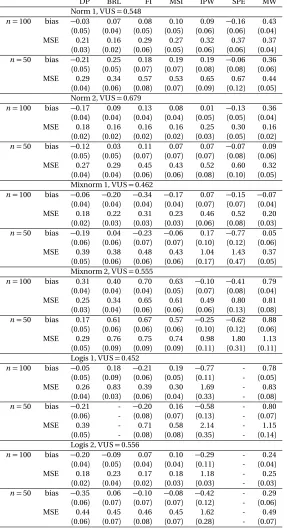
4.5 Simulations . . . 77
4.5.1 Nonparanormality assumption satisfied . . . 78
4.5.2 Nonparanormality assumption fails . . . 81
4.6 Real data . . . 82
LIST OF TABLES
Table 2.1 Bias(×10)and MSE(×102)for VUS estimates,L1-distances(×10)and L∞-distances between the estimated ROC surface and the true ROC surface without verification bias, VUS=0.671. . . 24 Table 2.2 Bias(×10)and MSE(×102)for VUS estimates,L1-distances(×10)and
L∞-distances between the estimated ROC surface and the true ROC surface under verification bias. . . 26 Table 2.3 Bias(×10)and MSE(×102)for VUS estimates,L1-distances(×10)and
L∞-distances between the estimated ROC surface and the true ROC surface when departing from the trinormality assumption,n=(200, 200, 200), VUS=0.358. . . 27 Table 2.4 Bias(×10)and MSE(×102)for VUS estimates,L
1-distances(×10)and L∞-distances between the estimated ROC surface and the true ROC
surface when departing from the MAR assumption,n=(200, 200, 200), VUS=0.671. . . 28
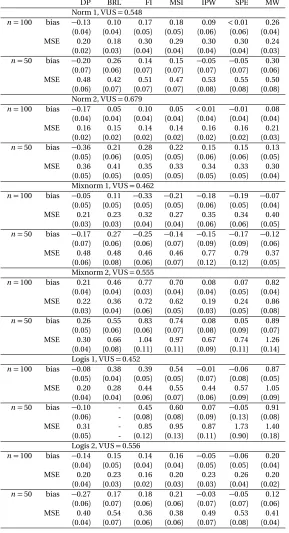
Table 3.1 Bias (×10) and MSE (×102) for the estimate of the VUS, with verifica-tion bias generated using the threshold model,n=100 and 50. (DP: Dirichlet Process, BRL: Bayesian Rank Likelihood, FI: Full Imputation, MSI: Mean Score Imputation, IPW: Inverse Probability Weighted, SPE: Semi-Parametric Efficient, MW: Mann-Whitney U-statistic) . . . 51 Table 3.2 Bias (×10) and MSE (×102) for the estimate of the VUS, with
verifi-cation bias generated using the probit model,n =100 and 50. (DP: Dirichlet Process, BRL: Bayesian Rank Likelihood, FI: Full Imputation, MSI: Mean Score Imputation, IPW: Inverse Probability Weighted, SPE: Semi-Parametric Efficient, MW: Mann-Whitney U-statistic) . . . 52 Table 3.3 Bias (×10) and MSE (×102) for the estimate of the VUS, with
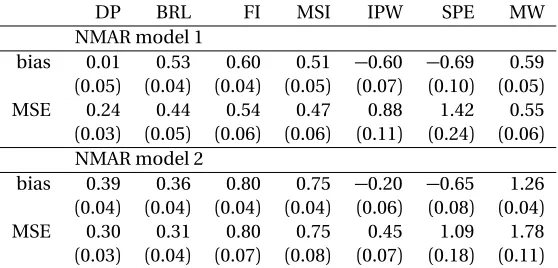
verifica-tion bias departing from NMAR model,n=100. (DP: Dirichlet Process, BRL: Bayesian Rank Likelihood, FI: Full Imputation, MSI: Mean Score Imputation, IPW: Inverse Probability Weighted, SPE: Semi-Parametric Efficient, MW: Mann-Whitney U-statistic) . . . 53 Table 3.4 Bias (×10) and MSE (×102) for the estimate of the VUS without
Table 4.1 Classification error rate (×102) for the test data when the data is gener-ated with a logistic transformation. (Here * means there are 1–6 cases failed to output a result. The error is calculated based on the remianing outputs.) . . . 79 Table 4.2 Classification error rate (×102) for the test data when the data is
gener-ated with a probit transformation. (Here * means there are 1–6 cases failed to output a result. The error is calculated based on the remianing outputs.) . . . 80 Table 4.3 Classification error rate (×102) for the test data when the data violate
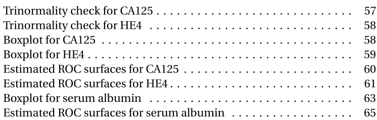
LIST OF FIGURES
Figure 3.1 Trinormality check for CA125 . . . 57
Figure 3.2 Trinormality check for HE4 . . . 58
Figure 3.3 Boxplot for CA125 . . . 58
Figure 3.4 Boxplot for HE4 . . . 59
Figure 3.5 Estimated ROC surfaces for CA125 . . . 60
Figure 3.6 Estimated ROC surfaces for HE4 . . . 61
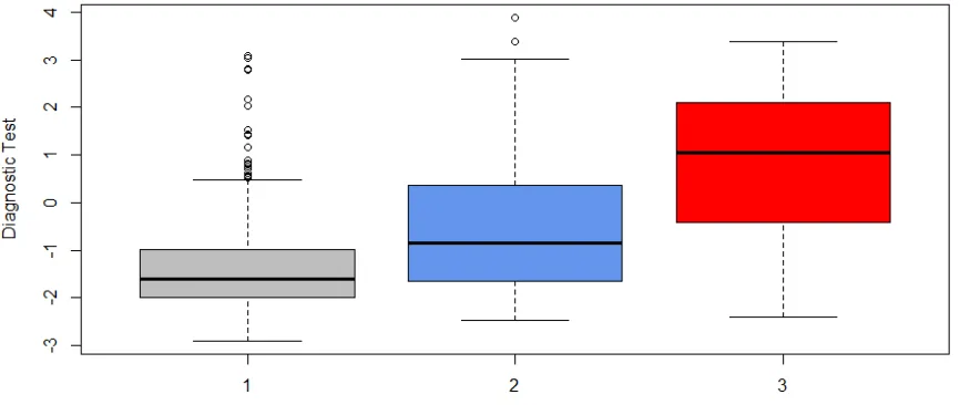
Figure 3.7 Boxplot for serum albumin . . . 63
CHAPTER
1
INTRODUCTION
Semi-supervised learning is a classification method which makes use of both labeled data
and unlabeled data for training. There has been a growing interest in semi-supervised
learning in recent years. Traditional classification methods are supervised in nature. They
use only labeled data for training. To train a traditional classifier, we have to obtain the true
class information for each unit in the dataset, along with the measurements associated with
it. However, labels are often difficult to obtain. It can be expensive and time consuming,
and it requires human labor and expertise. On the other hand, unlabeled data in most cases
are substantial and easy to obtain. Unsupervised learning methods like clustering provide
a way to make use of unlabeled data. However, it may not be appropriate or useful in a
When a few units in a dataset have labels, then semi-supervised learning technique can
use these large number of unlabeled units in classification instead of discarding them; thus
greatly improves the performance of the classifier. In summary, semi-supervised learning
lies in between supervised learning and unsupervised learning and the goal is to make
most efficient use with a dataset containing both labeled and unlabeled observations.
Semi-supervised learning can be classified to two big classes – generative methods and
discriminative methods. Generative methods are mainly based on Expectation-Maximization
(EM) algorithm (Dempster et al. 1977) and they have to make some assumptions on the
underlying distributions of different classes. Discriminative methods, on the other hand,
only learn the boundary between classes. In the recent literature, discriminative methods
are explored much more compared to generative methods. Self-Training (Yarowsky 1995) is
the most widely-used semi-supervised learning method. The basic idea is that the chosen
classifier teaches itself the labels and then learn iteratively. Co-Training (Blum and Mitchell
1998) is conducted by splitting the features to two subsets. The idea is that each subsets
can learn and teach the other some labels they are confident of. Another commonly used
algorithm is Semi-Supervised Support Vector Machines(S3VM). The goal of S3VM is to
find a linear boundary which has the maximum margin for both labeled and unlabeled
data. This is an NP-hard problem and there are many algorithms being proposed to solve
this problem. The method S3VM is based on the assumption that the boundary will not
cut in dense regions. Other methods like Gaussian Process (Lawrence and Jordan 2005)
also make use of this assumption. There are also a huge number of methods based on
graphical analysis, like Balcan et al. (2009); Zemel and Carreira-Perpiñán (2005); Zhang
and Lee (2007); Hein and Maier (2007) etc. A thorough introduction of semi-supervised
learning methods can be found in Zhu (2005).
In this thesis, we will focus on generative methods to solve semi-supervised learning
Chap-ter 4. Before considering a general semi-supervised learning algorithm, we will first consider
one specific application of semi-supervised learning-the Receiver Operating Characteristic
(ROC) surface estimation under verification bias, in Chapter 2 and 3.
So what is ROC surface? An ROC surface is a natural generalization of an ROC curve
which is intended to evaluate the classifier for three-class classification problem (Scurfield
1996). It plots the True Class Fractions (TCFs) in three axes respectively, and thus illustrates
the trade-off among the three TCFs as the cut-off points vary. Analogous to the AUC for ROC
curve, the volume under the surface (VUS) is proposed as a measure of the accuracy for
three-dimensional classifiers, which can be calculated by integrating out the ROC surface.
One common problem in the data that complicates the ROC surface estimation is called
verification bias. In reality, the true class each individual belongs to may not be completely
known to us. In biomedical settings, for example, we want to estimate the accuracy of a
biomarker in distinguishing healthy patients, early phase patients and late phase patients
for certain disease. We can use ROC surface for this purpose. Here the class may be the
true disease status of the patient, which is usually verified through a gold standard test,
the perfect existing diagnostic test. However, such a test may be expensive and invasive.
It is more ethical to apply a gold standard test only to those high risk subjects according
to the screening test. This leads to the problem of missing data. Because patients who are
marked as low-risk are more likely to have their true disease status missing, simply ignoring
this missingness and estimating the ROC surface using only subjects with verified disease
status may lead to biased results, and will cause a loss of efficacy (quantitative measure
of the effectiveness of the test) as well. The same problem can happen when evaluating a
classification algorithm. Since labeled data are hard to obtain, we can face the situation
when we do not have enough labeled data to evaluate an algorithm. We definitely would
like to use unlabeled data as well if possible to evaluate the algorithm in these cases.
of semi-supervised learning since both of them want to study the underlying distributions
when true labels are partially known. We choose to start with this particular application first
since the data for estimating ROC surface is univariate, which is easier to handle even though
three classes are in present instead of two. We consider two different approaches to solve
the problem of estimating the ROC surface. In Chapter 2, we propose a semi-parametric
Bayesian method based on continuous data under a semi-parametric trinormality
assump-tion. That is, we assume that under some unknown transformation, the data from three
categories follow three different normal distributions. The posterior distribution is
com-puted using a rank-based likelihood and the consistency of the posterior under a mild
condition is established. In Chapter 3, we consider a Bayesian nonparametric method by
directly modeling the underlying distributions of the three categories by Dirichlet Process
mixture priors. With no assumption on the distributions, this method is even more robust.
Moreover, this method can accommodate covariates information in estimating the ROC
surface as well, which can lead to a more comprehensive understanding of the diagnostic
accuracy. Both methods can be adapted to the case where there is no verification bias. For
the second method, it can be adapted and hugely simplified in the case where there is no
verification bias, and very fast computation is possible through the Bayesian bootstrap
process. Both methods are compared with other commonly used methods by extensive
simulations. We find that the proposed methods generally outperforms other approaches.
Applying the methods to two real datasets, the key findings are as follows: (i) HE4 has a
slightly better diagnosis ability compared to CA125 in discriminating healthy, early stage
and late stage patients of epithelial ovarian cancer. (ii) Serum albumin has a prognostic
ability in distinguishing different stages of hepatocellular carcinoma.
In Chapter 4, we propose a general generative semi-supervised learning algorithm.
Un-like most generative methods, which are mainly based on Expectation-Maximization (EM)
Like in Chapter 2, we assume that the observations will follow two multivariate normal
distributions depending on their true labels after the same unknown transformation.
In-stead of getting rid of the unknown transformation using a rank likelihood, here we have to
explicitly put a prior on the transformation and average out with respect to its posterior
distribution. To do that, we use B-splines on each component of the transformation. The
function estimation is then reduced to the problem of estimation which we can impose
Gaussian priors with an ordering constraint. The posterior distributions can be calculated
using the Gibbs sampling framework to update the parameters. The proposed method is
then compared with several other state-of-art methods in extensive simulation studies and
real data application. We find that our proposed method has better prediction accuracy for
CHAPTER
2
BAYESIAN SEMIPARAMETRIC
ESTIMATION OF ROC SURFACE UNDER
VERIFICATION BIAS
2.1
Introduction
The Receiver Operating Characteristic (ROC) curve analysis has been widely used as an
effective tool in measuring the accuracy of diagnostic tests in the two-class classification
through all possible values of the diagnostic marker. Recently some surfaces related to the
ROC curve have been proposed for practical use (Martos and de Carvalho 2018; de Carvalho
et al. 2013). One of the most commonly used surface among them is called ROC surface.
The ROC surface is a generalization of the ROC curve for classification problems of three
outcomes. LetX,Y andZ be continuous measurements from three different classes,X ∼F0 are measurements from Class 0,Y ∼F1are measurements from Class 1, andZ ∼F2are measurements from Class 2. Suppose that the ordering of interest for these three classes
isX <Y <Z. A decision rule that classifies subjects can be defined by using two ordered
threshold pointsc1<c2, i.e. choose Class 0 when a measurement is less thanc1, choose
Class 1 when it is betweenc1andc2, and choose Class 2 otherwise. This will result in three
True Class Fractions (TCFs):
TCF0=P(X ≤c1) =F0(c1),
TCF1=P(c1≤Y ≤c2) =F1(c2)−F1(c1), TCF2=P(Z >c2) =1−F2(c2).
Varyingc1andc2will give us a set of TCFs. To construct the ROC surface, we plot(TCF0, TCF1,
TCF2)in a three-dimensional coordinate system. The functional form of the ROC surface
can be obtained by expressing TCF1as a function of(TCF0, TCF2)given by (Nakas and
Yiannoutsos 2004)
ROCs(TCF0, TCF2) =F1(F2−1(1−TCF2)−F1(F0−1(TCF0))). (2.1)
assessment of the diagnostic accuracy. The VUS is given by
VUS=
Z 1
0
Z 1−F2(F0−1(p0))
0
ROCs(p0,p2)d p2d p0;
see Nakas and Yiannoutsos (2004). This can be shown to be equal to P(X <Y <Z)(Mossman
1999).
The ROC surface has been used in diagnostic testing in medical sciences when the
disease has two phases, for example, the early phase and late phase of a progressive disease.
The symptoms in the early phase may be mild and ignorable, while the late phase tends to
have more severe symptoms. Clearly, there is an inherent ordering between healthy, early
phase diseased and late phase diseased. One example is Alzheimer’s disease, which can be
graded low, intermediate and high according to the progress of the disease (Chi and Zhou
2008). Different medical treatments should be applied to different phases. The treatment
for the late phase of the disease can be expensive and invasive to patients, even requiring
surgeries, while the treatment for the early phase can be conservative. This necessitates the
identification of the two phases of the disease and thus leads to the consideration of three
classes. We assume, without loss of generality, that a higher test value indicates a higher
level of disease.
Many methods have been proposed for estimating the ROC surface. The empirical
estimator of ROC surface was obtained by simply replacing the cumulative distribution
functions in (2.3) by their empirical estimators (Li and Zhou 2009), and VUS can be
cal-culated by integrating out this ROC estimator. Another empirical estimator was given by
the unbiased nonparametric Mann-Whitney U statistic of the probability P(X <Y <Z)
(Dreiseitl et al. 2000), which was later extended to the case with ties (Nakas and Yiannoutsos
2004). Kang and Tian (2013) proposed using Gaussian kernel approaches for estimation of
based on Finite Pólya Tree prior distributions was proposed by Inácio et al. (2011).
A parametric method of estimating the ROC surface is based on the parametric
trinor-mality assumption:X ∼N(µ0,σ2
0),Y ∼N(µ1,σ12),Z ∼N(µ2,σ22), where N(µ,σ
2)denotes the
normal distribution with meanµand varianceσ2. Xiong et al. (2006) obtained a closed
form expression of the ROC surface under this assumption. If the data are not normally
distributed, Kang and Tian (2013) proposed using the Box-Cox transform. Li and Zhou
(2009) introduced two semi-parametric estimators of the ROC surface by extending the
methods of Hsieh and Turnbull (1996) and Nze Ossima et al. (2015) for estimating the ROC
curve.
In this chapter, we propose a new semiparametric method for estimating the ROC
surface. This is a generalization of a Bayesian method for estimating the ROC curve using a
rank-based likelihood (BRL) introduced by Gu and Ghosal (2009). We assume that, under
some unknown strictly monotone increasing transformation, the measurements follow
three different normal distributions. Since ranks are invariant under a strictly monotone
increasing transformation, exploiting the rank-likelihood eliminates the need for estimating
the unknown transformation, and enable us to construct a Bayesian estimator of ROC
surface.
We shall also consider the possibility of verification bias in the data which widely occurs
in practice but is rarely considered in the existing literature. That is to say, the true labels of
the subjects are partially missing. As we introduced in Chapter 1, this is a common problem
in the biomedical setting, where the label of a subject refers to the true disease status. Since
label is verified only through a very accurate existing diagnostic test called a gold standard
test, which is usually expensive and can even be invasive, the common practice is to apply
it only on high-risk subjects identified through a screening test. Because patients who are
marked as low-risk are more likely to have their true disease status missing, simply ignoring
status may lead to biased results, and will cause a loss of efficacy as well.
So to deal with the missing labels, the commonly used missing at random (MAR)
assump-tion (Little and Rubin 2014) will be adopted. The assumpassump-tion means that the probability
of a subject being verified does not depend on the disease status given the observed
mea-surements. This is reasonable in biomedical contexts since the decision to obtain the gold
standard test is generally made by looking at the diagnostic test results and other
exter-nal factors, while the effect of the true disease status is already incorporated through its
influence in diagnostic tests.
The existing literature is very limited for this problem. Chi and Zhou (2008) obtained the
maximum likelihood estimator for the ROC surface and the VUS for ordinal diagnostic tests.
To Duc et al. (2016) considered this problem for continuous diagnostic tests. They proposed
several bias-corrected estimators of TCFs and thus constructed several bias-corrected ROC
surfaces. These methods are extensions of Full Imputation (FI), Mean Score Imputation
(MSI), Inverse Probability Weighted (IPW), Semi-Parametric Efficient (SPE) estimators
for the ROC curves in Alonzo and Pepe (2005). They chose a suitable parametric model
to compute the probability of each individual belonging to each class based on verified
subjects, and then applied this model to unverified subjects. They also used a suitable
parametric model to compute the probability of verification. These probabilities are used
to adjust for the influence caused by missing labels.
Through some modifications, our method for estimating the ROC surface can be
ex-tended to the setting under verification bias. This can also be regarded as a generalization
of the ROC curve estimation under verification bias proposed by Gu et al. (2014). Covariates
are not considered in our formulation. If additional covariates information is available, it
may be used to model disease prevalence rates(λ0,λ1,λ2)of the three levels, by
multicate-gory logistic regression, for instance. This will make the classification probabilities (2.10)
not pursue this proposed method in this Chapter.
The chapter is organized as follows. The methodology is described in Section 2.2 and
2.3. We first consider the setting without verification bias and then consider the case under
verification bias. A result on consistency of the posterior distribution obtained from the
rank likelihood is presented in Section 2.4. Extensive simulation studies are conducted in
Section 2.6. The proposed Bayesian rank likelihood method will be applied to a real data
set in the next chapter after introducing another method of estimating ROC surface under
verification bias. The proof of the posterior consistency result is given in the appendix.
Because the methods in Chapter 3 are proposed for the same purpose, we will apply the
two methods along with other methods on a real data in Chapter 3.
2.2
Method for fully verified data
We first consider the setting without verification bias. The diagnostic measurements for
allN subjects in the study is denoted byS=(S1, . . . ,SN)and their true disease status are
denoted byD= (D1, . . . ,DN), whereDi =0 means healthy,Di=1 means level-1 diseased
group andDi=2 means level-2 diseased group. As we observe the true disease status, the
ith subject can be labeled simply asLi =Di,i =1, . . . ,N. LetL= (L1, . . . ,LN). So we have
n0=P1{Di =0}observations from healthy group,n1=
P
1{Di =1}observations from
level-1 disease group andn2=P1{Di=2}observations from level-2 diseased group.
LetF0,F1andF2be the underlying continuous cumulative distribution functions of the
diagnostic measurements for healthy group, level-1 diseased group and level-2 diseased
group respectively, so that
Based on the trinomality assumption, under some strictly monotone increasing
transfor-mationH, the transformed observationsQi=H(Si),i =1, . . . ,N, satisfy
Qi|{Di=k}
i.i.d.
∼ N(µk,σ2k), k =0, 1, 2, (2.2)
for someµ0< µ1< µ2andσ0,σ1,σ2 >0. To ensure the identifiability of the model, the
distribution of the middle group (without loss of generality) has been set to be the standard
normal (i.e.µ1=0,σ1=1). Nevertheless, to unify certain formulas for different groups, we
shall occasionally use the notations(µk,σk),k=0, 1, 2, with the interpretation thatµ1=0
andσ1=1. Note that sinceH is unknown,Q=H(S)is unobservable.
Since the ROC function remains unchanged under monotonic transformations, it is
immediate that the ROC function in the semiparametric trinormal model coincides with
that of the parametric trinormal model, admitting the explicit functional form (Xiong et al.
2006)
R(x,y) =
ΦΦ−1(1−y) +d
c
−ΦΦ
−1(x) +b
a
+
, (2.3)
whereΦ(·)denote the cumulative distribution function of N(0, 1), the plus sign stands for the positive part and
a =1/σ0, b =µ0/σ0, c =1/σ2, d =µ2/σ2. (2.4)
The volume under the ROC surface (VUS) is given by
VUS=
Z ∞
−∞
Φ(a s−b)Φ(−c s+d)φ(s)d s, (2.5)
on(µ0,σ0,µ2,σ2). This is especially convenient in the Bayesian setting since Markov chain
Monte Carlo (MCMC) algorithms can easily sample from the posterior distribution of
(µ0,σ0,µ2,σ2)through a data augmentation technique, to be below.
It is hard to get an assessment of(µ0,σ0,µ2,σ2)beforehand as there are no direct
obser-vations from the corresponding normal populations. Following Gu et al (2014), we consider
the standard improper prior densityπ(µ0,σ0,µ2,σ2)∝σ0−1σ−21 for the locational-scale parameters but restrict to the regionµ0<0< µ2. As the effect of the unknown transformH
has been eliminated, we do not need a prior distribution onH.
SinceH is a strictly monotone increasing transformation,R(Q), the ranks ofQpreserve
those ofS. The rank-likelihood is therefore given by the probability thatQmaintains these
observed ranking, as a function of the parameters(µ0,σ0,µ2,σ2). The numerical evaluation
of the likelihood is expensive because it involves computing the probability of a cone
defined by ordering in a high dimensional normal distribution. On the other hand, the
simple restriction that theith smallest entry ˜Qi ofQlies between ˜Qi−1 and ˜Qi+1allows
sampling the latent variablesQin a Gibbs sampling framework, making the Bayesian
computation much more feasible than obtaining the maximum likelihood estimates. With
the knowledge of the rank vectorR, clearlyQcan be recovered from the ordered values
˜
Q= (Q˜1, . . . , ˜QN).
LetSeandQestand for the order statistics ofSandQrespectively. BecauseH is a strictly
monotone increasing function, we haveQe=H(Se). In addition, letLeandDfstand for the
label and the true disease status corresponding toQerespectively.
Posterior sampling can be done by Gibbs sampling. To start with, we need to specify the
initial value forQe, which must satisfy three conditions: (i) it has to be ordered; (ii) it must
have labels according toDf; (iii)Qi|{Di =1} ∼N(0, 1),i =1, . . . ,N. We consider using the
transformed value of observedSeas our initial value forQe. Transformation is needed
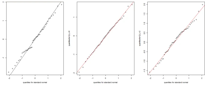
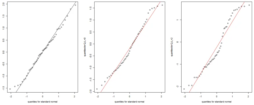
to be approximately normal, which can be checked using a Q-Q plot. Otherwise, we may
try some standard transformations first and check if the transformed data is approximately
normal. If this fails as well, we can use the Box-Cox transformation so that the transformed
value for the level-1 diseased group will be roughly N(0, 1). We can then generate the initial
value for(µ0,σ0,µ2,σ2)according to the initial value ofQe. Specifically,
µ0,0=
N
X
i=1
f
Qi1{Dfi=0}/n0, σ20,0=
N
X
i=1
(Qfi1{Dfi=0} −µ0,0)2/(n0−1),
µ2,0=
N
X
i=1
f
Qi1{Dfi=2}/n2, σ22,0= N
X
i=1
(Qfi1{Dfi=2} −µ2,0)2/(n2−1).
(2.6)
wheren0=
PN
i=11{Dfi=0},n2= PN
i=11{Dfi=2}. With those initial values, we shall calculate
the ROC surface based on posterior distributions of Gibbs sampling in Algorithm 1.
Algorithm 1Bayesian Rank Likelihood (BRL) without verification bias.
input :Df, initial valuesQe,(µ0,0,σ0,0,µ2,0,σ2,0),(n0,n1,n2), niter output :(µ0, σ0, µ2, σ2)
form←1toniterdo fori ←1toN do
e
Qi|{Dei=k}, rest∼TN(µk,m−1,σ2k,m−1,(Qei−1,Qei+1)) end
¯ En0=
PN
i=1Qfi1{Dfi=0}/n0
s2
0 =
PN
i=1(Qfi1{fDi=0} −E¯n0)2/(n0−1)
¯ Gn2=
PN
i=1Qfi1{fDi=2}/n2 s2
2 =
PN
i=2(Qfi1{Dfi=2} −G¯n2)
2/(n2−1)
σ2
0,m|rest∼IG((n0−1)/2,(n0−1)s
2 0/2)
µ0,m|rest∼TN(E¯n0,σ
2
0,m/n0,(−∞, 0))
σ2
2,m|rest∼IG((n2−1)/2,(n2−1)s22/2)
µ2,m|rest∼TN(G¯n2,σ
2
2,m/n2,(0,∞))
Notice that in the algorithm, the symbol niter is the total number of iterations in the
MCMC algorithm, TN stands for truncated normal distribution, IG stands for inverse
gamma distribution, and thatQe0,m =−∞,QeN+1,m=∞,µ1,m =0,σ1,m=1,m =0, . . . , niter.
In each iteration, we get(µ0,m,σ0,m,µ2,m,σ2,m),m=1, . . . , niter. We can calculate(am,bm,
cm,dm)for each iteration according to (2.4) and VUSm according to (2.5). Monitoring the
convergence through trace plot and discarding all samples for a suitable burn-in period,
we can obtain the estimated parametric ROC surface estimates according to the sample
mean of the parameters(a,b,c,d). The VUS can be also estimated by averaging out the
computed value VUSm in each MCMC iteration.
2.3
Method in presence of verification bias
Under verification bias, only a fraction of patients go through the gold standard test and
have their true disease statusDi observed,i =1, . . . ,N, soL= (L1, . . . ,LN)is different from
the previous case. IfDi is obtained, i.e., the true disease status is known, the labelLi=Di;
otherwise we setLi=3, indicating the absence of applying a gold standard test. ThusLi
indicates missing status as well as true disease status if the latter is actually observed.
Under verification bias, the number of patients in each disease group is unknown.
Assume that, the disease prevalence rates for level-1 and level-2 in the population are
λ1 and λ2 respectively. So the number of patients in each group follows (n0,n1,n2) ∼ Mult(N,(λ0,λ1,λ2)), where Mult stands for the Multinomial distribution,λ0=1−λ1−λ2, 0< λ1<1, 0< λ2<1, and 0< λ1+λ2<1.
Because of the existence of verification bias, we need to build a model for observing
labels, i.e., going through the gold standard test. In a clinical practice, the gold standard test
will typically be prescribed according to the screening test results. To be specific, a subject
likely to take the gold standard test. Because of this, missing completely at random may
not be appropriate. Simply ignoring unverified subjects will lead to a biased estimation.
Here we follow Gu et al. (2014) and model this as missing at random. In general, this model
of verifying disease status can be represented as
P(Li6=3|Qi,Di) =g(Qi), (2.7)
for a given monotone increasing functiong.
There are reasonable missing mechanisms which follow (2.7). In a scheme proposed
by Alonzo and Pepe (2005), verification is mandatory for the topp1fraction according to
the diagnostic test, while it is done with probabilityp2for the remaining subjects, where
0<p1,p2<1 are chosen beforehand. Since the ordering will not change under the monotone
transformationH,Qs andSs share the same ordering, this can be considered as a special
case of (2.7) with
g(Q) =
1, ifQ>Q(p1N),
p2, ifQ≤Q(p1N).
(2.8)
This verification mechanism will be called threshold model later in the simulation part. If a
probit regression model is followed for verification,
g(Q) =Φ(α+βQ), (2.9)
whereα,β are known parameters withβ >0. Notice that the case without verification bias
can be regarded as a special case of (2.7) by simply settingg(Qi) =1.
We adopt a Bayesian approach to estimate(λ1,λ2,µ0,σ0,µ2,σ2). We again use the
im-proper priorπ(µ0,σ0,µ2,σ2)∝σ−1
1 σ−
1
distribu-tion,α0,α1andα2are chosen according to the mean and standard error from our prior
knowledge.
If theith subject is unverified, its disease statusDigiven the latent variableQi follows
the probability distribution given by Lemma 2.5.1, namely,
P(Di=k|Qi=t,Li=3) =λkφ(µk,σk)(t)/∆(t) =pk(t), (2.10)
say, where∆(t) =P2
k=0λkφ(µk,σk)(t)andφ(µ,σ)(·)denote the density function of N(µ,σ
2). A
remarkable feature in our modeling using the MAR assumption is that the expression in
(2.10) does not depend on the verification functiong, allowing us to compute the posterior
distribution without actually knowingg. Thus, this method is guarded against
misspecifi-cation in the verifimisspecifi-cation model, and is more robust compared with other methods which
focus on the verification probability.
To obtain samples from the posterior distribution, additionally we need to consider the
collection of unobserved status asDun={Di:Li=3,i ≤N}as latent variables and apply
Gibbs sampling with these variables augmented withθ= (λ1,λ2,µ0,σ0,µ2,σ2,Qe). Then
givenDun, sampling from the posterior distribution ofθis exactly as in the case without
verification bias; when givenθ, the posterior sampling ofDunfollows from (2.10). For the
initial values, first we need to specify the initial values for unobservedDi’s, i.e.,Di∈Dun. We samplefDi∼Mult(1,(λ0,λ1,λ2))ifLei=3,i =1, . . . ,N, where(λ0,λ1,λ2)are sampled from Dir(α0,α1,α2). The initial values can then be generated exactly as previously introduced.
With those initial values, we can obtain the ROC surface as in Algorithm 2.
As in the previous algorithm, we haveQe0,m =−∞,QeN+1,m = ∞,µ1,m =0,σ1,m = 1,
m=0, . . . , niter. We can calculate(am,bm,cm,dm)according to(µ0,m,σ0,m,µ2,m,σ2,m),m=
1, . . . , niter for each iteration. Monitoring the convergence through trace plot and discarding
estimates according to the sample mean of the parameters(a,b,c,d). The VUS is also
estimated by averaging out the computed value VUSm in each MCMC iteration.
2.4
Posterior consistency
As the case without verification bias can be regarded as a special case of under verification
bias model by simply settingg(Qi) =1 in (2.7), we only need to show posterior consistency
under verification bias.
Letνdenote the Lebesgue measure andπdenote the prior density for(µ0,σ0,µ2,σ2)
with respect toν. Let(µ∗
0,σ∗0,µ∗2,σ∗2)be the true value of(µ0,σ0,µ2,σ2), that is, the parameter value responsible for the data generating process. The following says that for most values of
(µ∗
0,σ
∗
0,µ
∗
2,σ
∗
2), the posterior concentrates around the true value in large samples, providing a theoretical justification of the proposed method from the frequentist point of view.
Theorem 2.4.1 Assume that (2.2) and (2.7) hold for a monotone increasing function g :R→ (0, 1)andπ(µ0,σ0,µ2,σ2)>0a.e.[ν]onR−×R+×R+×R+. Then for(µ∗0,σ0∗,µ∗2,σ∗2)a.e.[ν], and any neighborhoodU0of(µ∗0,σ0∗,µ∗2,σ∗2), we have that
lim
N→∞Π((µ0,σ0,µ2,σ2)∈ U0|R(S),L) =1,a.s. (2.11)
with respect to[P∞ µ∗
0,σ∗0,µ∗2,σ∗2,g,H], the true joint distribution of all ranks and labels.
Since(a,b,c,d)is a continuous reparameterization of(µ0,σ0,µ2,σ2), it is immediate
that the induced posterior of(a,b,c,d)is also consistent for almost all of its true values.
Clearly, as the ROC surface and the VUS function depend continuously on(a,b,c,d), these
objects are also consistently estimated by the proposed Bayesian method.
We prove Theorem 2.4.1 using a general posterior consistency theorem by Doob. The
pre-sented in Ghosal and van der Vaart (2017). We show that the vector of parameters can
be expressed as a function of the observations and then apply Doob’s theorem to show
posterior consistency.
While Theorem 2.4.1 does not give posterior consistency at all possible true values of
the parameter, the assertion is still very attractive as the possible exceptional set where
convergence may fail has Lebesgue measure zero, meaning it is a “small set" that “can be
ignored". This is a lot more useful than the conclusion generally obtained from Doob’s
theorem which characterizes the exceptional set as only having measure zero with respect
to the prior, and hence is “small" only in a “subjective sense". In contrast, the “objectivity" of
the exceptional set in our setting is obtained because we can effectively treat the parameter
space as Euclidean (where there is a prior density which can be chosen to be positive
throughout the parameter space). This is because the procedure does not depend on the
transformation functionH and the verification functiong, and hence these can be treated
as fixed.
2.5
Lemmas and proofs
The following lemma gives the probability distribution of the disease status when
unob-served, conditional on the latent measurementQ introduced in the trinormal model.
Lemma 2.5.1 Let S1, ...,SN be the independent diagnostic variables with underlying disease
status D1, ...,DN, where Di∈ {0, 1, 2}for i =1, . . . ,N ,P(Di=k) =λk, k=0, 1, 2whereλ0+λ1+
λ2=1. Let S|{D=k} ∼fk, k=0, 1, 2, and L=D if D is observed and L=3otherwise. Assume
that verification bias follows MAR assumption as in Eq. 2.7. Then
P(Di =k|Si=t,Li=3) =P(Di=k|Si=t,Li6=3) =
λkfk(t)
where f(t) =λ0f0(t) +λ1f1(t) +λ2f2(t).
Proof By Bayes’s theorem,
P(Di=k|Si=t,Li=3) ==
λkfk(t)(1−g(t))
P2
l=0λlfl(t)(1−g(t))
= λkfk(t)
P2
l=0λlfl(t) ,
and P(Li=3)is given by
2
X
k=0
Z
P(Li=3,Di=k|Si=t)fk(t)d t =
2
X
k=0
λk
Z
fk(t)(1−g(t))d t.
In Chapter 2, fk =φ(µk,σk2). The following lemma will be needed in the proof of the
consistency theorem in 2.4.1.
Lemma 2.5.2 In the setup of Lemma 2.5.1, the conditional density of Q given that L6=3is given by fQ(t|L6=3) =
P2
k=0λ∗kφ(∗µk,σk,g), where for k =0, 1, 2,
λ∗
k=
λk
R
g(s)φ(µk,σk)(s)d s P2
l=0λl
R
g(s)φ(µl,σl)(s)d s
, φ(µ,σ,g)(t) =R g(t)φ(µ,σ)(t)
g(s)φ(µ,σ)(s)d s
. (2.13)
Proof By an application of Bayes’s theorem, we evaluate fQ(t|L6=3)as
P(L6=3|Q=t)P2k=0P(D =k)φ(µk,σk)(t) R
P(L6=3|Q=s)P2
k=0P(D =k)φ(µk,σk)(s)d s
= g(t) P2
k=0λkφ(µ1,σ1)(t)
R
g(s)P2k=0λkφ(µ1,σ1)(s)d s
=
2
X
k=0
g(t)φ(µk,σk)(t) R
g(s)φ(µk,σk)(s)d s
× λk R
g(s)φ(µk,σk)(s)d s P2
l=0λl
R
g(s)φ(µl,σl)(s)d s
= 2 X k=0 λ∗ kφ ∗
(µk,σk,g)(t).
on them. Hence we can treat g andH as known to prove consistency of the posterior
distribution of(µ0,σ0,µ2,σ2).
We verify the conditions of Doob’s Theorem as presented by Ghosal and van der Vaart
(2017), Theorem 6.9 and Proposition 6.10. Let the set of all permutations of{1, . . . ,N}be denoted byΩN. We need to show the existence of a functionh∗:Ω
1×Ω2×· · ·×{0, 1, 2, 3}∞→
R−×R+×R+×R+, such that(µ0,σ0,µ2,σ2) =h∗(RN,N ≥1,(L1,L2, . . .))a.s.
Let 1≤i1 <· · ·<iN∗ ≤N be all indices withLij =0, 1 or 2, j =1, ...,N
∗. Disregarding
the information on the true disease status, by Lemma 2.5.2, the correspondingQ values
are generated from the mixture distributionQij
i.i.d.
∼ P2
k=0λ∗kΦ(µk,σk,g) whereΦ ∗
(µ,σ,g) is the cumulative distribution function ofφ∗
(µ,σ,g). Thus we have
Uj∗= 2
X
k=0
λ∗
kΦ(µk,σk,g)(Qij)
i.i.d.
∼ Uniform(0, 1).
Let (R0
N∗1, . . . ,RN0∗N∗) and(LN0 ∗1, . . . ,L0N∗N∗)be the rank vector and labels of(U1∗, . . . ,UN∗∗)
re-spectively. According to Theorema on page 157 of Hájek and Šidák (1967), we have
E
Uj∗−
RN0∗
i j
N∗+1 2
= 1
N∗
N∗
X
k=1
EUj∗− k
N∗+1 2
|RN0∗
i j =k = 1 N∗ N∗ X k=1
k(N∗−k+1) (N∗+1)2(N∗+2)<
1 N∗,
so E U∗ j − R0 N∗ i j
N∗+1 2
→0 asN → ∞becauseN∗/N converges to a positive limit, there exists
a subsequence{N∗
k}of{N∗}such that forj ≥1,Uj∗=limk→∞(Nk∗+1)
−1R0
N∗
ki j a.s. Thus we can
writeU∗
j =hj(RN,N ≥1,L1,L2, . . .)for some functionhj :Ω1×Ω2× · · · × {0, 1, 2, 3}∞→[0, 1]. Now given {Qij : Lij = 1}
i.i.d.
∼ Φ∗
(0,1,g), so that {Uj∗ : Lij = 1}
i.i.d.
∼ V(µ0,σ0,µ2,σ2,g), where
V(µ0,σ0,µ2,σ2,g)is the distribution of
P2
k=0λ∗kΦ∗(µk,σk,g)(ξ), withξ∼Φ ∗
(0,1,g). Since(Uj∗:Lij =1)are
es-timable. Thus we only need to show that the family of{V(µ0,σ0,µ2,σ2,g):µ0<0< µ2,σ0>0,σ2>
0}is identifiable, i.e., ifV(µ0,σ0,µ2,σ2,g)=V(µ00,σ00,µ02,σ20,g), then(µ0,σ0,µ2,σ2) = (µ
0
0,σ
0
0,µ
0
2,σ
0
2). To prove this, first we show thatΦ∗
(µ,σ,g)andΦ(∗µ0,σ0,g)are linearly independent whenever
(µ,σ)6= (µ0,σ0). If not, there exists somec
1,c2∈Rsuch thatc1Φ∗(µ,σ,g)(t)+c2Φ∗(µ0,σ0,g)(t) =0 for allt. By differentiation, we obtainc1φ∗(µ,σ,g)(t) +c2φ(∗µ0,σ0,g)(t) =0 for allt. Now asg(t)6=0 for allt, this leads toc1φ(µ,σ)(t) +c2φ(µ0,σ0)(t)for allt in view of the definition ofφ(µ,σ,g)(t).
This contradicts the obvious linear independence ofφ(µ,σ)andφ(µ0,σ0), two distinct normal
densities. The argument easily extends to finitely many distributions. Thus the assertion of
identifiability follows because of the restrictionsµ0<0 andµ2>0, which allow to separate
the roles of the two mixture components.
Therefore we conclude that for some functionh of(U1,U2, . . . ,L1,L2, . . .), and
conse-quently for a functionh∗of all ranks and labels, almsot surely we have
(µ0,σ0,µ2,σ2,g) =h(U1,U2, . . .)
=h(h1(RN,N ≥1,L1,L2, . . .),h2(RN,N ≥1,L1,L2, . . .), . . .)
=h∗(RN,N ≥1,L1,L2, . . .).
This verifies the condition of Doob’s theorem and hence posterior consistency holds at
almost every(µ∗0,σ∗0,µ∗2,σ∗2)with respect to the joint prior distribution of these parameters.
2.6
Simulation
2.6.1
Without verification bias
We first consider applying our method when there is no verification bias in the data. In
this simulation, letn = (n0,n1,n2), so we generaten0,n1andn2samples from N(−1.8, 1.52), N(0, 1)and N(2, 22)respectively, and then apply the inverse-transformH−1on them to obtain
the observable data. Note that by (2.3), the true value of(a,b,c,d)is(0.667,−1.2, 0.5, 1) and the corresponding value of the VUS is 0.671. We consider both balanced cases where
n= (50, 50, 50),(100, 100, 100)and an unbalanced case wheren= (100, 40, 20). We setn0>
n1>n2for the unbalanced case since in biomedical settings, there are much more healthy
patients than diseased patients. We consider two different true transformationsH here —
(i) logarithmic:H(x) =logx; (ii) logit transformation:H(x) =log(x/(1−x)).
We compare our method (BRL) with other existing methods. The first method, proposed
by Kang and Tian (2013) estimates the unknown transformationH parametrically from the
Box-Cox transformation family using the maximum likelihood method (Xiong et al. 2006),
and will be referred to as BC in the tables. Note that one of the true transformations we
consider, the logarithmic transformation, belongs to the Box-Cox transformation family.
We also compare BRL with two other semiparametric methods (denoted here by Semi1 and
Semi2) proposed by Li and Zhou (2009), which fit an ROC surface of the stated form under
the trinormality assumption to the empirical ROC surface estimate. Finally, we consider
comparing BRL to a non-parametric Bayesian surface estimate based on Finite Pólya Tree
prior distributions, proposed by Inácio et al. (2011), denoted as Pólya. The simulation
results for the bias and the MSE of the VUS estimates, and the averageL1-distances and
L∞-distances between the estimated surfaces and the true ROC surface are shown in Table
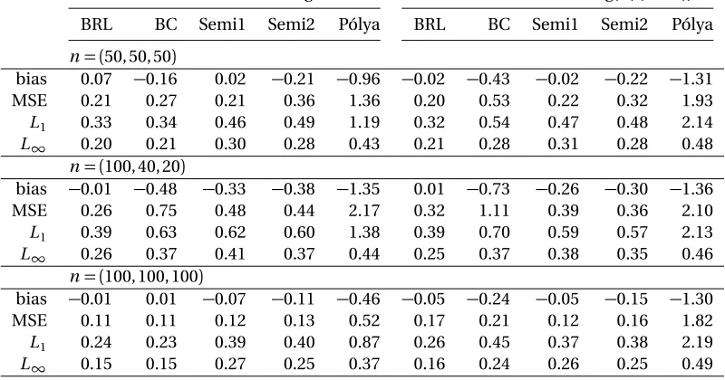
Table 2.1: Bias (×10) and MSE (×102) for VUS estimates, L1-distances (×10) and L
∞
-distances between the estimated ROC surface and the true ROC surface without verification bias, VUS=0.671.
True transformation=logx True transformation=log(x/(1−x)) BRL BC Semi1 Semi2 Pólya BRL BC Semi1 Semi2 Pólya
n= (50, 50, 50)
bias 0.07 −0.16 0.02 −0.21 −0.96 −0.02 −0.43 −0.02 −0.22 −1.31 MSE 0.21 0.27 0.21 0.36 1.36 0.20 0.53 0.22 0.32 1.93 L1 0.33 0.34 0.46 0.49 1.19 0.32 0.54 0.47 0.48 2.14
L∞ 0.20 0.21 0.30 0.28 0.43 0.21 0.28 0.31 0.28 0.48 n= (100, 40, 20)
bias −0.01 −0.48 −0.33 −0.38 −1.35 0.01 −0.73 −0.26 −0.30 −1.36 MSE 0.26 0.75 0.48 0.44 2.17 0.32 1.11 0.39 0.36 2.10 L1 0.39 0.63 0.62 0.60 1.38 0.39 0.70 0.59 0.57 2.13
L∞ 0.26 0.37 0.41 0.37 0.44 0.25 0.37 0.38 0.35 0.46 n= (100, 100, 100)
bias −0.01 0.01 −0.07 −0.11 −0.46 −0.05 −0.24 −0.05 −0.15 −1.30 MSE 0.11 0.11 0.12 0.13 0.52 0.17 0.21 0.12 0.16 1.82 L1 0.24 0.23 0.39 0.40 0.87 0.26 0.45 0.37 0.38 2.19
L∞ 0.15 0.15 0.27 0.25 0.37 0.16 0.24 0.26 0.25 0.49
Pólya methods are calculated with 90000 Gibbs samples (100000 MCMC iterations after
10000 samples used for burn-in). The biases shown in Table 2.1 are multiplied by 10, MSEs
are multiplied by 102,L
1-distances are multiplied by 10,L∞-distances are shown in the
original scale, for convenience of display. The same applies to the remaining tables.
From the tables above, we can conclude that BRL succeeds in almost every case
con-sidered. Relatively low bias and MSE suggest that the method has an accurate estimate
of VUS, while lowL1-distance andL∞-distance suggest that the estimated surface is very
close to the true ROC surface. The Box-Cox method also has a good performance when the
true transformation is logarithmic, which is expected since this transformation belongs to
the Box-Cox family, but not as good for the logit transformation. BRL, on the other hand,
is quite robust with respect to the true transformation, since the BRL method eliminates
the effect of the transformation through ranks. Semi1 has a relatively good performance in
more accurate estimates of the ROC surface and the VUS when the number of observations
doubled for the balanced case. For the unbalanced case, even though the total number of
patients actually increased slightly (from 150 to 160), the performances of most methods
are still worse compared with the balanced case whenn = (50, 50, 50).
2.6.2
Under the trinormality assumption with verification bias
In this simulation,n is set to be(100, 100, 100)for the balanced case and to(200, 150, 100)
for the unbalanced case. We consider two different trinormal distributions settings of
(µ0,σ0,µ2,σ2): (a)(−1.8, 1.5, 2, 2)and (b)(−3, 2, 2, 1), which respectively correspond to VUS values 0.671 and 0.833, and the underlying transformation is chosen to be the logit
trans-formation.
Within each simulation setting, consider two verification mechanisms: (i) threshold
model withp1=0.8,p2=0.4 in 2.8, and (ii) probit regression model withβ=1,α=0.106
in 2.9 for balanced cases;β=1,α=0.5 for the unbalanced cases of (a);β=1,α=1 for the
unbalanced cases of (b). Both schemes will generate about half of the missing labels. The
BRL estimates are obtained by 90000 Gibbs samples (100000 MCMC iterations after 10000
iterations used for burn-in). In total 100 datasets are simulated for the study.
There are only a few methods available to deal with data with verification bias for
esti-mating the ROC surface. We compare the proposed BRL method with Full Imputation (FI),
Mean Score Imputation (MSI), Inverse Probability Weighted (IPW), Semi-Parametric
Effi-cient (SPE) methods proposed by To Duc et al. (2016). We use a multivariate logistic model
to estimate the true disease rate and a logistic model to estimate verification rate in order
to apply those methods. We compare those methods in terms of the estimated accuracy of
the VUS, and also the averageL1-distance andL∞-distance between the estimated and
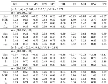
Table 2.2: Bias (×10) and MSE (×102) for VUS estimates, L1-distances (×10) and L∞
-distances between the estimated ROC surface and the true ROC surface under verification bias.
Threshold Probit
BRL FI MSI IPW SPE BRL FI MSI IPW SPE
(a,b,c,d) = (0.667,−1.2, 0.5, 1), VUS=0.671 n= (100, 100, 100)
bias 0.02 −0.39 −0.03 0.55 0.26 −0.37 −0.93 −0.83 −1.02 −1.07 MSE 0.22 0.52 0.29 0.54 0.32 0.50 1.59 1.45 2.79 2.39 L1 0.51 1.08 0.73 0.77 0.69 0.66 1.67 1.47 1.37 1.52
L∞ 0.20 0.36 0.29 0.39 0.31 0.22 0.54 0.47 0.47 0.49 n= (200, 150, 100)
bias −0.15 −0.31 −0.08 0.38 0.09 −0.59 −0.73 −0.62 −0.54 −0.69 MSE 0.15 0.44 0.30 0.48 0.43 0.55 0.75 0.60 0.80 0.87 L1 0.48 1.09 0.73 0.68 0.73 0.78 1.47 1.22 0.87 1.03
L∞ 0.18 0.42 0.32 0.36 0.34 0.24 0.52 0.42 0.34 0.35
(a,b,c,d) = (0.5,−1.5, 1, 2), VUS=0.833 n= (100, 100, 100)
bias −0.07 −0.38 −0.20 0.33 0.15 −0.38 −2.27 −2.22 −2.21 −2.17 MSE 0.12 0.40 0.23 0.20 0.14 0.37 6.55 6.36 8.70 6.35 L1 0.34 0.70 0.50 0.49 0.46 0.51 2.20 2.14 1.96 2.18
L∞ 0.20 0.27 0.24 0.34 0.29 0.23 0.48 0.49 0.54 0.53 n= (200, 150, 100)
bias −0.42 −0.56 −0.32 0.26 0.12 −0.64 −1.69 −1.59 −0.87 −1.39 MSE 0.26 0.49 0.23 0.13 0.09 0.52 3.16 2.80 1.08 2.21 L1 0.50 0.76 0.49 0.39 0.41 0.69 1.64 1.53 0.85 1.37
Table 2.3: Bias (×10) and MSE (×102) for VUS estimates, L1-distances (×10) and L
∞
-distances between the estimated ROC surface and the true ROC surface when departing from the trinormality assumption,n=(200, 200, 200), VUS=0.358.
Threshold Probit
BRL FI MSI IPW SPE BRL FI MSI IPW SPE
bias 0.10 0.47 0.25 0.13 −0.12 −0.14 0.46 0.23 −0.01 0.01 MSE 0.04 0.31 0.15 0.16 0.16 0.07 0.28 0.13 0.10 0.10 L1 0.74 0.61 0.42 0.48 0.45 0.61 0.57 0.38 0.39 0.39
L∞ 0.37 0.16 0.13 0.18 0.19 0.33 0.15 0.11 0.16 0.15
We can see that BRL almost always has the lowest bias and MSE for the VUS estimates,
and the lowestL1andL∞-distances. There are a few exceptions though. For example, for
the unbalanced case of(a,b,c,d) = (0.5,−1.5, 1, 2)where verification bias is generated using threshold model, IPW has lower bias and MSE for the VUS estimates, and lowerL1-distance
estimates as well. MSI estimates of the VUS are quite comparable to BRL in terms of bias
and MSE for(a,b,c,d) = (0.667,−1.2, 0.5, 1)setting, but the estimated ROC surfaces have larger distances to the true ROC surface. Overall, BRL has a satisfying performance for all
cases considered above.
2.6.3
Departure from the trinormality assumption with verification bias
It is important to study the performance of our method when the data does not satisfy
the trinormality assumption. Here we generate(X1, . . . ,Xn0)independently from Beta(3, 5),
(Y1, . . . ,Yn1)independently from Beta(2, 2), and(Z1, . . . ,Zn2)independently from Beta(5, 3),
wheren= (200, 200, 200). The corresponding VUS=0.358 and 100 simulated data sets are
used in the study. For the verification bias models, we use the threshold mechanism with
p1=0.8 andp2=0.4, and the probit regression mechanism withα=0.01 andβ=0.07. Both
of them generate approximately half of the missing labels. The BRL estimates are obtained