PROTEIN SECONDARY STRUCTURE PREDICTION FROM
AMINO ACID SEQUENCE USING ARTIFICIAL
INTELLIGENCE TECHNIQUE
(MERAMAL STRUKTUR PROTEIN SEKUNDER DARI
JUJUKAN ASID AMINO MENGGUNAKAN TEKNIK
KEPINTARAN BUATAN)
SAFAAI BIN DERIS ROSLI BIN MD ILLIAS
SAHIDAN BIN SENAFI SAAD OSMAN ABDALLA SATYA NANDA VEL ARJUNAN
RESEARCH VOT NO: 74017
Jabatan Kejuruteraan Perisian
Fakulti Sains Komputer Dan Sistem Maklumat Univerisit Teknologi Malaysia
ii
ABSTRACT
ABSTRAK
iv
TABLE OF CONTENTS
CHAPTER TITLE PAGE
ABSTRACT
iiABSTRAK
iiiTABLE OF CONTENTS
ivLIST OF TABLES
xLIST OF FIGURES
xiiLIST OF ABBREVIATIONS
xvLIST OF APPENDICES
xviii1
INTRODUCTION
11.1 Introduction 1
1.2 Protein Structure Prediction 2
1.3 Prediction Methods 3
1.4 The Problem 6
1.5 Objectives of the Research 7
1.6 The Scope of the Research 8
1.7 Organization and Overview of the Report 8
1.8 Summary 10
2
PROTEIN, SEQUENCES, AND SEQUENCE
ALIGNMENT
11
2.1 Introduction 11
2.2 Proteins 11
2.2.1 Protein Primary Structure 15
2.2.3 Tertiary Structure 17
2.2.4 Quaternary Structure 18
2.3 Methods of Determining Protein Structure 18 2.4 Characteristics of Protein Structures 20
2.5 Protein Homology 21
2.5.1 Types of Homologies 22
2.5.2 Homologues versus Analogues 22 2.6 Molecular Interactions of Proteins 23
2.7 Sequence Alignment Methods 24
2.7.1 Threading Methods 24
2.7.2 Hidden Markov Models 25
2.7.3 Types of Alignment Methods 26 2.7.3.1 Pairwise Alignment Methods 27 2.7.3.2 Profile Alignment Methods 29 2.7.3.3 Multiple Alignment Methods 30
2.7.4 Comparative Modelling 32
2.7.5 Overview of Alignment Methods and Programs
33
2.8 Summary 35
3
REVIEW OF PROTEIN SECONDARY
STRUCTURE PREDICTION: PRINCIPLES,
METHODS, AND EVALUATION
36
3.1 Introduction 36
3.2 Protein Secondary Structure Prediction 38 3.3 Methods Used In Protein Structure Prediction 40
3.4 Artificial Neural Networks 47
3.4.1 Inside the Neural Networks 47
3.4.2 Feedforward Networks 49
3.4.3 Training the Networks 51
3.4.4 Optimization of Networks 52
3.5 Information Theory 54
3.5.1 Mutual Information and Entropy 55
vi Folding Problem
3.5.3 GOR Method for Protein Secondary Structure Prediction
59 3.6 Data Used In Protein Structure Prediction 61 3.7 Prediction Performance (Accuracy) Evaluation 63
3.7.1 Average Performance Accuracy (Q3) 64
3.7.2 Segment Overlap Measure (SOV) 65
3.7.3 Correlation 65
3.7.4 Receiver Operating Characteristic (ROC) 66 3.7.5 Analysis of Variance Procedure (ANOVA) 67
3.8 Summary 68
4
METHODOLOGY
704.1 Introduction 70
4.2 General Research Framework 70
4.3 Experimental Data Set 74
4.4 Hardware and Software Used 75
4.5 Summary 76
5
A METHOD FOR PROTEIN SECONDARY
STRUCTURE PREDICTION
USING NEURAL NETWORKS AND GOR-V
77
5.1 Introduction 77
5.2 Proposed Prediction Method – NN-GORV-I 78
5.2.1 NN-I 78
5.2.2 GOR-IV 78
5.2.3 Multiple Sequence Alignments Generation 79
5.2.4 Neural Networks (NN-II) 81
5.2.4.1Mathematical Representation of Neural Networks
81
5.2.4.2Generating the Networks 86
5.2.4.3Networks Optimization 88
5.2.4.4Training and Testing the Network 89
5.2.6 NN-GORV-I 94 5.2.7 Enhancement of Proposed Prediction Method
- N-GORV-II
100
5.2.8 PROF 102
5.3 Reduction of DSSP Secondary Structure States 103 5.4 Assessment of Prediction Accuracies of the Methods 105 5.4.1 Measure of Performance (QH, QE, QC, and
Q3)
105
5.4.2 Segment Overlap (SOV) Measure 106
5.4.3 Matthews Correlation Coefficient (MCC) 106 5.4.4 Receiver Operating Characteristic (ROC) 107
5.4.4.1Threshold Value 109
5.4.4.2Predictive Value 109
5.4.4.3Plotting ROC Curve 110
5.4.4.4Area Under Curve (AUC) 110
5.4.5 Reliability Index 112
5.4.6 Test of Statistical Significance 112
5.4.6.1The Confidence Level (P-Value) 113
5.4.6.2Analysis of Variance (ANOVA)
Procedure
114
5.5 Summary 114
6
ASSESSMENT OF THE PREDICTION
METHODS
116
6.1 Introduction 116
6.2 Data Set Composition 117
6.3 Assessment of GOR IV Method 118
6.4 Assessment of NN-I Method 122
6.5 Assessment of GOR-V Method 123
6.6 Assessment of NN-II Method 126
6.7 Assessment of PROF Method 128
6.7.1 Three States Performance of PROF Method 130 6.7.2 Overall Performance and Quality of PROF
Method
132
6.8 Assessment of NN-GORV-I Method 134
viii Method
6.8.2 Overall Performance and Quality of NN-
GORV-I Method
139
6.9 Assessment of NN-GORV-II Method 140
6.9.1 Distributions and Statistical Description of NN-GORV-II Prediction
140 6.9.2 Comparison of NN-GORV-II Performance
with Other Methods
143 6.9.3 Comparison of NN-GORV-II Quality with
Other Methods
148 6.9.4 Improvement of NN-GORV-II Performance
over Other Methods
151 6.9.5 Improvement of NN-GORV-II Quality over
Other Methods
155 6.9.6 Improvement of NN-GORV-II Correlation
over Other Methods
156
6.10 Summary 158
7
THE EFFECT OF DIFFERENT REDUCTION
METHODS
160
7.1 Introduction 160
7.2 Effect of Reduction Methods on Dataset and Prediction
161
7.2.1 Distribution of Predictions 162
7.2.2 Effect of Reduction Methods on Performance 166 7.2.3 Effect of Reduction Methods on SOV 169 7.2.4 Effect of Reduction Methods on Matthews’s
Correlation Coefficients
171
7.3 Summary 173
8
PERFORMANCE OF BLIND TEST
1748.1 Introduction 174
8.2 Distribution of CASP Targets Predictions 175 8.3 Performance and Quality of CASP Targets
Predictions
179
8.4 Summary 183
9
RECEIVER OPERATING CHARACTERISTIC
(ROC) TEST
184
9.2 Binary Classes and Multiple Classes 185
9.3 Assessment of NN-GORV-II 189
9.4 Summary 193
10
CONCLUSION
19410.1 Introduction 194
10.2 Summary of the Research 195
10.3 Conclusions 197
10.4 Contributions of the Research 199 10.5 Recommendations for Further Work 199
10.6 Summary 201
REFERENCES
202APPENDIX A (PROTEIN STRUCTURES ) 230 APPENDIX B (CUFF AND BARTON’S 513
PROTEIN DATA SET)
233
x
LIST OF TABLES
TABLE NO. TITLE PAGE
2.1 The twenty types of amino acids that forms the proteins 12
2.2 The standard genetic code 14
3.1 Well established protein secondary structure prediction methods with their reported accuracies and remarks briefly describing each method.
46
5.1 The contingency table or confusion table for ROC curve 108 5.2 ANOVA table based on individual observations (One
way ANOVA)
114
6.1 Total number of secondary structures states in the data base
118
6.2 The percentages of prediction accuracies with the standard deviations of the seven methods
120
6.3 The SOV of prediction accuracies with the standard deviations of the seven methods
121
6.4 The Mathew’s correlation coefficients of predictions of the seven methods
122
6.5 Descriptive Statistics of the prediction accuracies of NN-GORV-II method
142
6.6 Descriptive Statistics of the prediction of SOV measure for NN-GORV-II method
142
6.7 Percentage Improvement of NN-GORV-II method over the other six prediction methods
152
6.8 SOV percentage improvement of NN-GORV-II method over the other prediction methods
6.9 Matthews Correlation Coefficients improvement of NN-GORV-II method over the other six prediction methods
157
7.1 Percentage of secondary structure state for the five reduction methods of DSSP definition (83392 residues)
162
7.2 The analysis of variance procedure (ANOVA) of the Q3
for the five reduction methods
163
7.3 The analysis of variance procedure (ANOVA) of SOV for the five reduction methods
164
7.4 The effect of the five reduction methods on the performance accuracy of prediction (Q3)the of
NN-GORV-II prediction method
167
7.5 The effect of the five reduction methods on the segment overlap measure (SOV)of the NN-GORV-II prediction method
169
7.6 The effect of reduction methods on Matthews’s
correlation coefficients using NN-GORV-II prediction method
172
8.1 Percentages of prediction accuracies for the 42 CASP3 proteins targets
180
8.2 Percentages of SOV measures for the 42 CASP3 proteins targets
181
8.3 The mean of Q3 and SOV with and standard deviation, and Mathew’s Correlation Coefficients (MCC) of CASP
182
9.1 The contingency table or confusion matrix for coil states prediction
187
9.2 The cut scores for the NN-GORV-II algorithm considering coil only prediction
189
9.3 The cut scores, true positive rate (TPR), false positive rate (FPR), and area under ROC (AUC) for the NN-GORV-II prediction algorithm considering coil state only prediction
xii
LIST OF FIGURES
FIGURE NO. TITLE PAGE
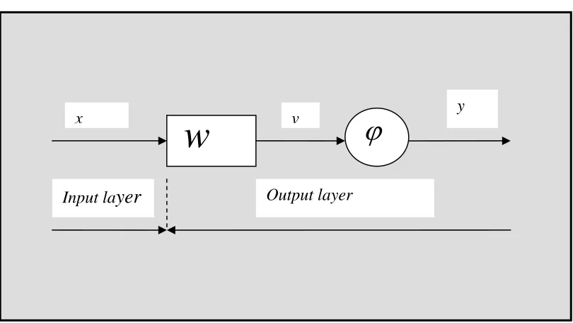
3.1 Basic graphical representations of a block diagram of a single neuron artificial neural networks.
48
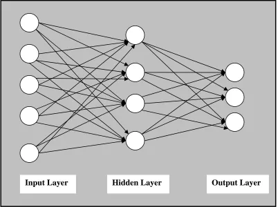
3.2 Representation of multilayer perceptron artificial neural networks.
50
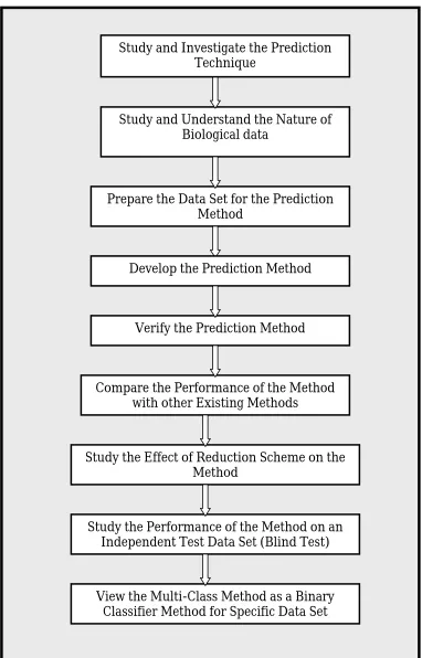
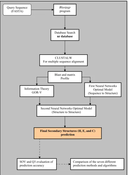
4.1 General framework for protein secondary structure prediction method
72
4.2 An example of a flat file of CB513 data base used in this research, 1ptx-1-AS.all file.
75
5.1 Basic representation of multilayer perceptron artificial neural network
82
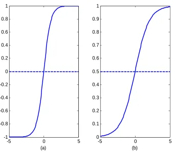
5.2 The sigmoidal functions usually used in the feedforward Artificial Network. (a) Hyperbolic tangent sigmoid transfer function or bipolar function (b) Log sigmoid transfer function or uniploar function
83
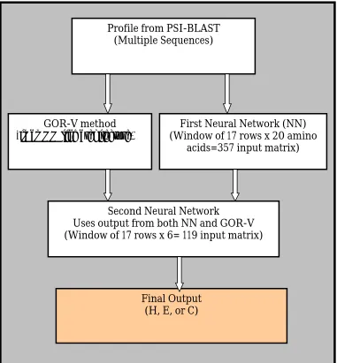
5.3 A general model for the newly developed protein secondary structure prediction method.
95
5.4 A detailed representation for the first version of the newly developed protein secondary structure prediction method (NN-GORV-I)
96
5.5 A detailed representation for the second version of the newly developed protein secondary structure prediction method (NN-GORV-II)
101
5.6 The 1ptx-1-AS.all file converted into a FASTA format (zptAS.fasta) readable by the computer programs.
104
the Q3 and SOV program
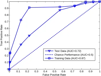
5.8 A typical example of area under curve (AUC) for training data, test data, and chance performance or random guess
111
6.1 The performance of the GOR-IV prediction method with respect to Q3 and SOV prediction measures
119
6.2 The performance of the NN-I prediction method with respect to Q3 and SOV prediction measures
123
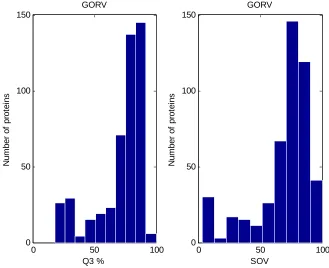
6.3 The performance of the GOR-V prediction method with respect to Q3 and SOV prediction measures
124
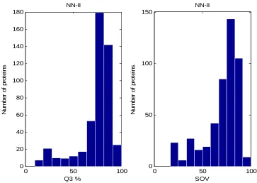
6.4 The performance of the NN-II prediction method with respect to Q3 and SOV prediction measures
127
6.5 The performance of the PROF prediction method with respect to Q3 and SOV prediction measures
129
6.6 The α helices performance (QH) of the seven prediction
methods
130
6.7 The βstrands performance (QE) of the seven prediction
methods
130
6.8 The coils performance (QC) of the seven prediction
methods
132
6.9 The performance of the NN-GORV-I prediction method with respect to Q3 and SOV prediction measures
135
6.10 The helices segment overlap measure (SOVH) of the
seven prediction methods
137
6.11 The strands segment overlap measure (SOVE) of the
seven prediction methods
137
6.12 The coils segment overlap measure (SOVC) of the seven
prediction methods
138
6.13 The performance of the NN-GORV-II prediction
method with respect to Q3 and SOV prediction measures
xiv 6.14 Histogram showing the Q3 performance of the seven
prediction methods
144
6.15 A graph line chart for the Q3 performance of the seven
prediction methods.
147
6.16 Histogram showing the SOV measure of the seven prediction methods
148
6.17 A graph line chart for the SOV measure of the seven prediction methods
150
7.1 Five histograms showing the Q3 distribution of the test proteins with respect to the five reduction methods
165
7.2 Five histograms showing the SOV distribution of the test proteins with respect to the five reduction methods
166
7.3 The performance accuracy (Q3) of the five reduction
method on the test proteins
168
7.4 The SOV measure of the five reduction method on the 480 proteins using NN-GORV-II prediction method
171
8.1 The distribution of prediction actuaries of the of the 42 Casp targets blind test for the secondary structure states.
176
8.2 The performance of the 42 CASP targets with respect to Q3 and SOV prediction measures
177
8.3 The distribution of SOV measure of the of the 42 Casp targets blind test for the secondary structure states.
178
9.1 An idealized curve showing the (TP, TN, FP, and FN) numbers of a hypothetical normal and Not normal observations
188
9.2 The cut scores of the coils and not coils secondary structure states predicted by the NN-GORV-II algorithm using Method V reduction scheme.
190
9.3 The area under ROC (AUC) for the NN-GORV-II prediction algorithm considering coil only prediction.
LIST OF ABBREVIATIONS
1D - One Dimensional Protein Structure 3D - Three Dimensional Protein Structure HGP - Human Genome Project
GenBank - Gene Bank
PDB - Protein Data Bank
EMBL - European Molecular Biology Laboratory
DNA - Deoxyribonucleic Acid
RNA - Ribonucleic Acid
mRNA - Messenger RNA
NMR - Nuclear Magnetic Resonance
GOR - Garnier-Osguthorpe-Robson
BLAST - Basic Local Alignment Search Tool PSIBLAST - Position Specific Iterated Blast ROC - Receiver Operating Characteristic AUC - Area Under Curve
NN-GORV-I - Neural Network GOR V Version 1 Prediction Method NN-GORV-II - Neural Network GOR V Version 2 Prediction Method Q3 - Prediction Accuracy of Helices, Strands, And Coils
QH - Prediction Accuracy of Helix State
QE - Prediction Accuracy of Strand State
QC - Prediction Accuracy of Coil State
SOV3 - Segment Overlap Measure Of Helices, Strands, And Coils
SOVH - Segment Overlap Measure Of Helix State
SOVE - Segment Overlap Measure Of Strand State
SOVC - Segment Overlap Measure Of Coil State
MCC - Matthews Correlations Coefficient
NN - Neural Network
xvi RF - Radio Frequency Pulses
CE - Combinatorial Extension
FSSP - Database F Families Of Structurally Similar Proteins SCOP - Structural Classification Of Proteins
HMMs - Hidden Markov Models
FASTA - Fast Alignment
GenThreader - Genomic Sequences Threading Method MSA - Multidimensional Sequence Alignments PRINTS - Protein Fingerprints
PRODOM - Protein Domain
PROF - Profile Alignment
PSSM - Position Specific Scoring Matrix PRRP - Prolactin-Releasing Peptide SCANPS - Protein Sequence Scanning Package PHD - Profile Network From Heidelberg
DSSP - Dictionary Of Protein Secondary Structure Prediction SAM - Sequence Alignment Method
MULTALIGN - Multiple Alignment
MULTAL - Multiple Alignment
HMMT - Hidden Markov Model Training For Biological Sequences BAliBASE - Benchmark Alignments Database
PIM - Protein Interaction Maps ITERALIGN - Iteration Alignment MLP - Multi-Layer Perceptron MI - Mutual Information
H - α Helix
E - β Strand
C - Coil
CPU - Central Processing Unit
RCSB - Research Collaboratory For Structural Bioinformatics PDB - Protein Data Bank
3Dee - Database Of Domain Definitions (DDD) CB513 - Cuff And Barton 513 Proteins
TP - True Positive
TN - True Negative
FP - False Positive
FN - False Negative
ANOVA - Analysis Of Variance nr - Non Redundant Database
PERL - Practical Extraction And Reporting Language
RES - Residues
LMS - Least Mean Square
SNNS - Stuttgart University Neural Network Simulator ANSI - American National Standards Institute
RI - Reliability Index FTP - File Transfer Protocol
SPSS - Statistical Package For Social Sciences SAS - Statistical Analysis Software
SE - Standard Error
xviii
LIST OF APPENDICES
APPENDIX TITLE PAGE
A Protein Structures 230
B Cuff and Barton’s 513 Protein Data Set 233
C Descriptive Statistics 244
CHAPTER 1
INTRODUCTION
1.1 Introduction
Advances in molecular biology in the last few decades, and the availability of equipment in this field have allowed the increasingly rapid sequencing of considerable genomes of several species. In fact, to date, several bacterial genomes, as well as those of some simple eukaryotic organisms (e.g. yeast) have been completely sequenced. The Human Genome Project (HGP), aimed to sequence all of the human chromosomes, is almost completed with a rough draft announced in the year 2000 (Heilig et al., 2003). Known sequencing databases projects, such as
GenBank, PDB, and EMBL, have been growing significantly. This surge and overflow of data and information have imposed the rational storage, organization and indexing of sequence information.
Explaining the tasks undertaken in Bioinformatics field in details might be far beyond this introductory chapter. However, they fall in the creation and maintenance of databases of biological information with nucleic acid or protein sequences cover the majority of such databases. Storage and organization of millions of nucleotides is essential portion in these databases. Designing, developing, and implementing databases access and exchange information between researchers in this field is progressing significantly.
2
of a protein using algorithms that have been derived from the knowledge of physics, chemistry and from the analysis of other proteins with similar amino acid sequences. Some researchers refer to this area with the name Computational Biology.
1.2 Protein Structure Prediction
Protein structure prediction is categorized under Bioinformatics which is a broad field that combines many other fields and disciplines like biology, biochemistry, physics, statistics, and mathematics. Proteins are series of amino acids known as polymers linked together into contiguous chains. In a living cell the DNA of an organism encodes its proteins into a sequence of nucleotides (transcribed), namely: adenine, cytosine, guanine and thymine that are copied to the mRNA which are then translated into protein (Branden and Tooze, 1991)
Protein has three main structures: primary structure which is essentially the linear amino acid sequence and usually represented by a one letter notation. Alpha helices, beta sheets, and loops are formed when the sequences of primary structures tend to arrange themselves into regular conformations; these units are known as secondary structure (Pauling and Corey, 1951; Kendrew, 1960). Protein folding is the process that results in a compact structure in which secondary structure elements are packed against each other in a stable configuration. This three-dimensional structure of the protein is known as the protein tertiary structure. However, loops usually serve as connection points between alpha-helices and beta-sheets, they do not have uniform patterns like alpha-helices and beta-sheets and they could be any other part of the protein structure rather than helices or strands (Appendix A).
In the molecular biology laboratory, protein secondary structure is determined experimentally by two lengthy methods: X-ray crystallography method and Nuclear Magnetic Resonance (NMR) spectroscopy method.
information must be somehow specified by the primary protein sequence, researchers have been trying to predict secondary structure from protein sequence. Anfinsen’s hypothesis suggests that an ideal theoretical model of predicting protein secondary structure from its sequence should exist anyhow.
1.3 Prediction Methods
There are two main different approaches in determining protein structure: a molecular mechanics approach based on the assumption that a correctly folded protein occupies a minimum energy conformation, most likely a conformation near the global minimum of free energy. Potential energy is obtained by summing the terms due to bonded and non-bonded components estimated from these force field parameters and then can be minimized as a function of atomic coordinates in order to reach the nearest local minimum (Weiner and Kollman, 1981; Weiner et al., 1984).
This approach is very sensitive to the protein conformation of the molecules at the beginning of the simulation.
One way to address this problem is to use molecular dynamics to simulate the way the molecule would move away from that initial state. Newton’s laws and Monte Carlo methods were used to reach to a global energy minima. The approach of molecular mechanics is faced by problems of inaccurate force field parameters, unrealistic treatment of solvent, and spectrum of multiple minima (Stephen et al.,
1990).
The second approach of predicting protein structures from sequence alone is based on the data sets of known protein structures and sequences. This approach attempts to find common features in these data sets which can be generalized to provide structural models of other proteins. Many statistical methods used the different frequencies of amino acid types: helices, strands, and loops in sequences to predict their location. (Chou and Fasman, 1974b; Garnier et al., 1978; Lim, 1974b;
4
segment or motif of a target protein that has a sequence similar to a segment or motif with known structure is assumed to have the same structure. Unfortunately, for many proteins there is no enough homology to any protein sequence or of known structure to allow application of this technique.
The previous review leads us to the fact that the approach of deriving general rules for predicting protein structure from the existing data sets or databases and then applies them to sequences of unknown structure appears to be promising. Several methods have utilized this approach (Richardson, 1981; Chou and Fasman, 1974a; Krigbaum and Knutton, 1973; Qian and Sejwaski, 1988; Crick, 1989).
Artificial Neural networks have great opportunities in the prediction of proteins secondary structures. These methods are based on the analogy of operation of synaptic connections in neurons of the brain, where input is processed over several levels or phases and then converted to a final output. Since the neural network can be trained to map specific input signals or patterns to a desired output, information from the central amino acid of each input value is modified by a weighting factor, grouped together then sent to a second level (hidden layer) where the signal is clustered into an appropriate class.
Artificial Neural Networks are trained by adjusting the values of the weights that modify the signals using a training set of sequences with known structure. The neural network algorithm adjusts the weight values until the algorithm has been optimized to correctly predict most residues in the training set.
Thus, neural networks and specially feedforward networks have a fair chance to well suite the empirical approach to protein structure prediction. In the process of protein folding, which is effectively finding the most stable structure given all the competing interactions within a polymer of amino acids, neural networks explore input information in parallel style.
The GOR method was first proposed by (Garnie et al., 1978) and named after
its authors Garnier-Osguthorpe-Robson. The GOR method attempts to include information about a slightly longer segment of the polypeptide chain. Instead of considering propensities for a single residue, position-dependent propensities have been calculated for all residue types. Thus the prediction will therefore be influenced not only by the actual residue at that position, but also to some extent by other neighbouring residues (Garnier and Robson, 1989). The propensity tables to some extent reflect the fact that positively charged residues are more often found in the C-terminal end of helices and that negatively charged residues are found in the N-terminal end.
The GOR method is based on the information theory and naive statistics. The mostly known GOR-IV version uses all possible pair frequencies within a window of 17 amino acid residues with a cross-validation on a database of 267 proteins (Garnier
et al., 1996). The GOR-IV program output gives the probability values for each
secondary structure at each amino acid position. The GOR method is well suited for programming and has been a standard method for many years.
The recent version GORV gains significant improvement over the previous versions of GOR algorithms by combining the PSIBLAST multiple sequence alignments with the GOR method (Kloczkowski et al., 2002). The accuracy of the
6
1.4 The Problem
The problem of this research focuses on the protein folding dilemma. The question is how protein folds up to its three dimensional structure (3D) from linear sequences of amino acids? The 3D structure protein is the protein that interacts with each other 3D protein and then produces or reflects functions. By solving the protein folding problem we can syntheses and design fully functioning proteins on a computational machine, a task that may requires several years in the molecular biology labs. A first step towards that is to predict protein secondary structures (helices, strands, and loops). At the time of writing this chapter, the prediction level of protein secondary structures is still at its slightly above the 70% range (Frishman, and Argos, 1997; Rost, 2001; Rost, 2003).
Prediction can not be completely accurate due to the facts that the assignment of secondary structure may vary up to 12% between different crystals of the same protein. In addition, β-strand formation is more dependent on long-range interactions than α-helices, and there should be a general tendency towards a lower prediction accuracy of β-strands than α-helices (Cline et al., 2002).
To solve the above mentioned problems, or in other words to increase the accuracy of protein secondary structure prediction, the hypothesis of this research can be stated as: “construction and designing advanced well organized artificial neural networks architecture combined with the information theory to extract more information from neighbouring amino acids, boosted with well designed filtering methods using the distant information in protein sequences can increase the accuracy of prediction of protein secondary structure”.
1.5 Objectives of the Research
amino acid sequence. However, the specific objectives of this research can be stated in the following points:
a. To analyse and study existing methods developed in the domain of protein secondary structure prediction to help in the development and implementation of a new prediction method.
b. To develop and implement a new accurate, robust, and reliable method to predict protein secondary structure from amino acid sequences.
c. To assess the performance accuracy of the method developed in this research and to compare the performance of the newly developed method with the other methods studied and implemented in this research work.
d. To study the differences between the secondary structure reduction methods and the effects of these methods on the performance of the newly developed prediction method.
e. To carry out blind test on the newly developed method. That is to analyse the output of the newly developed method with respect to an independent data set.
f. To study the performance of the coil prediction of the newly developed method using the ROC curve. This is also to examine the ability of ROC analysis to discriminate between two classes in a multi-class prediction classifier.
1.6 The Scope of This Research
8
clearly. The protein sequence data is obtained from the Cuff and Barton (1999) 513 protein database. The data is prepared from the Protein Data Bank (PDB) by Barton’s Group and considered as a benchmark sample that represents most PDB proteins. This study focuses on the neural networks and information theory since they are found to be effective for the prediction of protein secondary structure. The output results of the prediction methods are analysed and tested for performance, reliability, and accuracy. The limitation of this research work is the nature of the biological data which needs a great effort of pre-processing before the training and testing stages.
1.7 Organization and Overview of the Report
The organization and the flow of the contents of this report may be described as follows:
The report begins with Chapter 1 which we are reading now. The chapter explains key concepts, introducing the problem of this research, list the objectives, and determine the scope of this work.
Chapter 2 reviews and explains the proteins, sequences, and sequence alignments. It also examines amino acids and proteins in terms of their nature, formation, and their importance. The chapter reviews protein homology and homology detection and types of homologies proteins and then explains sequence alignment methods, pair-wise alignment, multiple alignments, as well as profile generation methods.
protein secondary structure with special emphasis to GOR theory. The tools and techniques used in this research as well as prediction performance evaluation procedures are introduced in this chapter..
Chapter 4 represents a brief and comprehensive methodology of this research. The chapter outlines and represents the framework followed in this research to implement the method proposed and developed in this research.
Chapter 5 represents and explains the modelling of the methodology and algorithms used to develop the new method NN-GORV-I and its advanced version NN-GORV-II. The data set for training and testing the newly developed methods beside the other methods that are implemented in this work was described. The implementation of PSIBLAST program search of the nr database to generate multiple
sequences which in turns are aligned by the CLUSTALW program is demonstrated in this chapter. The reduction methods used for the secondary structure data and the different statistical analysis and performance tests are demonstrated in this chapter.
Chapter 6 discusses the results of the seven different prediction methods developed or studied in this research. The Q3 , the segment
overlap (SOV) measure and the Matthews correlations coefficients MCC are discussed and examined in this chapter.
Chapter 7 discuses the effect of the five eight-to-three secondary structure reduction methods on the newly developed method in this research and trying to judge the argument that the eight-to-three state reduction scheme can alter the prediction accuracy of an algorithm.
10
predicted by the newly developed method to judge its performance and quality.
Chapter 9 introduces the Receiver Operating Characteristics (ROC) analysis and area under curve (AUC) to the newly method which is a multi-class classifier to estimate the prediction accuracy of the coil states.
Chapter 10 concludes and summarizes this research, highlights the contributions and findings of this work, and suggests some recommendations to further extend work.
1.8 Summary
CHAPTER 2
PROTEIN, SEQUENCES, AND SEQUENCE ALIGNMENT
2.1 Introduction
To grasp a better understanding to this research, a molecular biology introductory concepts and facts are inevitable. This chapter reviews in a comprehensive style the protein definition, nature, and it’s important to life. The chapter also explains the composition of proteins and its building blocks, the amino acids. The sequences and their alignments are discussed thoroughly in this review chapter. The different structures of proteins, methods of determining protein structure, and methods for generating homologue sequences and sequence alignment methods are presented in this chapter.
2.2 Proteins
12
The importance of sequence data can be used to make predictions of the functions of newly identified genes, estimate evolutionary distance in phylogeny, determine the active sites of enzymes, construct novel mutations and characterize alleles of genetic diseases. Sequence data also facilitates the analysis of the organization of genes and genomes and their evolution with respect to species and the identification of mutations that cause the diseases.
Multiple alignments of protein sequences are important tools in studying proteins. The basic information they provide is the identification of conserved sequence regions. This is very useful in designing experiments to test and modify the function of specific proteins, in predicting the function and structure of proteins, and in identifying new members of protein families (Durbin et al., 2002).
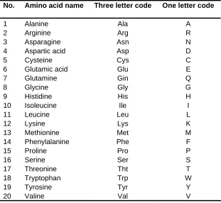
Proteins can be considered as series of amino acids linked together into contiguous chains. The 20 amino acids are shown in Table 2.1 with their respective three letter and one letter codes conventionally used in molecular biology.
Table 2.1: The twenty types of amino acids that forms the proteins
No. Amino acid name Three letter code One letter code
1 Alanine Ala A
2 Arginine Arg R
3 Asparagine Asn N
4 Aspartic acid Asp D
5 Cysteine Cys C
6 Glutamic acid Glu E
7 Glutamine Gin Q
8 Glycine Gly G
9 Histidine His H
10 Isoleucine Ile I
11 Leucine Leu L
12 Lysine Lys K
13 Methionine Met M
14 Phenylalanine Phe F
15 Proline Pro P
16 Serine Ser S
17 Threonine Tht T
18 Tryptophan Trp W
19 Tyrosine Tyr Y
In Bioinformatics research the one letter code is more commonly used than the three letter code. The training and testing protein sequences data used in this research adopts the one letter coding scheme.
The production of proteins in a cell is governed by codes and information transferred to the DNA, and RNA of the organism. Proteins are synthesized in the cells of living organisms, Prokaryotes (single cell) or Eukaryotes (high order) by a structured mechanism. The DNA of an organism encodes its proteins in a sequence of nucleotides, namely: adenine, cytosine, guanine and thymine. These nucleotides considered as information which is copied to the mRNA (messenger RNA) that serves as an intermediate medium, which is then processed during protein synthesis.
The codon (a non-overlapping triplet of nucleotides), specifies a corresponding subunit, or residue, to be added to the always growing polypeptide chain. The genetic code shown in Table 2.2 resembles the correspondence between the sequence of nucleotides of the codon and the amino acids which is constant in almost all organisms (Brian, 1998).
14
Table 2.2: The standard genetic code Second Position
T C A G
T
TTT Phe (F)
TTC Phe (F)
TTA Leu (L)
TTG Leu (L)
TCT Ser (S)
TCC Ser (S)
TCA Ser (S)
TCG Ser (S)
TAT Tyr (Y)
TAC Tyr (Y)
TAA Ter (end)
TAG Ter (end)
TGT Cys (C)
TGC Cys (C)
TGA Ter (end)
TGG Trp (W)
T C A G
C
CTT Leu (L)
CTC Leu (L)
CTA Leu (L)
CTG Leu (L)
CCT Pro (P)
CCC Pro (P)
CCA Pro (P)
CCG Pro (P)
CAT His (H)
CAC His (H)
CAA Gln (Q)
CAG Gln (Q)
CGT Arg (R)
CGC Arg (R)
CGA Arg (R)
CGG Arg (R)
T C A G
A
ATT Ile (I)
ATC Ile (I)
ATA Ile (I)
ATG Met (M)
ACT Thr (T)
ACC Thr (T)
ACA Thr (T)
ACG Thr (T)
AAT Asn (N)
AAC Asn (N)
AAA Lys (K)
AAG Lys (K)
AGT Ser (S)
AGC Ser (S)
AGA Arg (R)
AGG Arg (R)
T C A G F i r s t P o s i t i o n G
GTT Val (V)
GTC Val (V)
GTA Val (V)
GTG Val (V)
GCT Ala (A)
GCC Ala (A)
GCA Ala (A)
GCG Ala (A)
GAT Asp (D)
GAC Asp (D)
GAA Glu (E)
GAG Glu (E)
GGT Gly (G)
GGC Gly (G)
GGA Gly (G)
GGG Gly (G)
T C A G T h i r d P o s i t i o n
With the exception of proline, the amino acids described in Table 2.1 share the common feature of an amino and carboxyl group joined by a single carbon atom from which different side-chains are attached. However, glycine has no side-chain. Each type of amino acid has different side chain which gives it its distinguished characteristics. The peptide bond does not rotate freely, but the other two backbone bonds can rotate, allowing the polypeptide chain to fold in almost any direction.
2.2.1 Protein Primary Structure
The amino acid sequence is the primary structure of a protein. It is usually represented by the one letter notation of the amino acids. Amino acids combine to form a protein through polypeptide bonds and here the protein could be considered as polypeptide chain and the amino acids as residues (Table 2.1). Anyhow the reaction here is complex and lengthy to be mentioned in detail. A protein could be formed out of 2000 amino acids or residues although short chain proteins are not unusual. Shorter chains are called peptides. The different physical and chemical properties of the side-chains determine both the local and global conformations adopted by polypeptide chains. Anyhow the sequence direction is very important and usually represented from the amino, (N) terminus to the carboxyl (C) terminus.
2.2.2 Secondary Structure
The three-dimensional structure of proteins is potentially determined by its primary structure (Anfinsen, 1973), although the folding process can be aided by other molecules (Hartl, 1996). Most proteins always fold into the same configuration (Branden and Tooze, 1991).
Pauling and Corey (1951) predicted the existence of sheet-like structures of non-covalently cross-linked strands of extended polypeptide chain which they called beta-sheet and a helical arrangement. Studying the structures of myoglobin, Kendrew (1960) confirmed the existence of a regular helical arrangement, called alpha-helix. Alpha-helices and beta-sheets are the most common form of secondary structure in proteins.
16
Alpha-helix is spiral turns of amino acids while a beta-sheet is flat segments or strands of amino acids formed usually by a series of hydrogen bonds. As the polypeptide chain coils in, the CO and NH groups of residues form hydrogen bonds which stabilize the helix. Most of the residues in a helix are bonded in this way, making it somewhat a rigid unit of structure with a little free space in its core. A helix and can have 4 - 50 residues and makes a whole turn every 3.6 residues.
Beta-strands are the most regular form of extended polypeptide chain in protein structures. Like alpha-helices, beta-sheets are stabilized by hydrogen bonds between CO and NH groups, but they are distantly separated along the chain. Because of the geometry of the peptide backbone, the amino acid side chains of beta-strands alternate on either side of the sheet.
Loops usually serve as connection points between alpha-helices and beta-sheets, they do not have even patterns like alpha-helices and beta-sheets and they could be any other part of the protein structure. They are recognized as random coil and not classified as protein secondary structure. When the polypeptide chain makes very sharp changes in direction using as few as four residues by means of hydrogen bond, it forms turns. These secondary structures commonly contain proline or glycine or both residues (Hutchinson and Thornton, 1994).
2.2.3 Tertiary Structure
The three-dimensional structure of the protein, which is formed from the secondary structures as subunits elements, is known as the protein’s tertiary structure. Protein folding is the process that results in a compact structure in which secondary structure elements are packed against each other in a stable configuration. Dill (1990) reported that, the tendency for the burial of hydrophobic side-chains in the core of proteins has been observed in almost all structures discovered. It is believed this tendency is the driving force of tertiary structure formation.
Hydrogen bonds, van der Waals forces, and oppositely charged amino acid side-chains are other interactions that help to stabilize the fold. Folds are considered as sets of connected secondary structure elements, so they are known as topologies. Longer polypeptide chains that are usually clearly distinguished by a naked eye as self-contained units of structure, and have distinct hydrophobic cores, are known as domains. Swindells (1995), Islam et al. (1995), Siddiqui and Barton (1995) argued that the definition of domains is in this way is unreliable. A covalent linkage made during the folding process between sulphur atoms from cysteine residues is known as the disulphide bond (Freedman, 1995). Examples of proteins that exhibit disulphide are snake and scorpion toxins.
Levitt and Chothia (1976) grouped proteins into naturally four classes based upon the gross secondary structural content of their tertiary structures. These classes were: mainly-alpha, mainly-beta, alternating alpha-beta, and alpha and beta (not alternating). However, with the construction of a classified database of domains an automated approach to classification was developed (Michie et al., 1996).
18
2.2.4 Quaternary Structure
An individual protein that its independent fold or substructures form a three dimensional structure of the protein is known as quaternary structure. This is true for some proteins because they do not work in isolation; haemoglobin and RNA polymerase are examples of such proteins.
2.3 Methods of Determining Protein Structure
Three-dimensional structures of a protein can be determined by describing the relative position of a single atom within the protein using two laboratory methods: (i) X-ray crystallography and (ii) Nuclear Magnetic Resonance (NMR) spectroscopy. X-ray crystallography is the most popular method of protein structure determination. X-ray beams are applied to a crystal of proteins that has been grown by purifying a protein sample. The structure of the protein is then determined by studying the diffraction pattern of X-ray. Anyhow X-ray crystallography is a lengthy and complicated process; it requires a high level of technical ability in the laboratory reach to an inference of the x-ray diffraction patterns (Branden and Tooze, 1991).
Nuclear Magnetic Resonance (NMR) spectroscopy requires a highly concentrated and purified and a lowered pH sample of a protein. The protein is then put in a strong magnetic field, and subjected to radio frequency (RF) pulses. This will force the protein to emit RF radiation. Then information of protein structure can be inferred from the frequencies and intensities of the emitted radiation. Practically, this process is not as easy as been described and there are many biochemical constraints in this process (Branden and Tooze, 1991).
As far as hydrophobicity is concerned, many researchers identified the amino acids that commonly substitute with each other and categorized them with regard to their properties or structures and found that the most common clusters of a single column amino acid profiles were mostly hydrophobic or polar in nature (Han and Baker, 1995; Fiser et al., 1996; Ladunga and Smith, 1997).
The scale to measure hydrophobicity is not standardized and since it depends on the physico-chemical properties of amino acids, it was opened to subjective interpretations. However, Nakai et al. (1988), and Tomii and Kanehisa (1996) constructed a database of reported amino acids that shows their hydrophobicity scales and substitution matrices.
The distribution of disulphide bonds in cysteine residues stabilizes this amino acid and encodes important structural information since these bonds are mostly well conserved (Carrington and Boothroyd, 1996), while the distribution of cysteine residues does not encode important structural information in intracellular proteins interaction. However, pairwise interactions between distant homologues are not very well conserved (Russell and Barton, 1994).
20
2.4 Characteristics of Protein Structures
A protein could be subjected to denaturing forces like high temperature or low pH which force the protein to loose its original structure. Proteins tend to revert to their original structure, after the denaturing forces are removed. Anfinsen (1973) showed that the amino acid sequence is the only source of information to survive the denaturing process, so the structured information must be somehow specified by the sequence.
Many proteins exist in an aqueous solution within the cell, and certain amino acid side chains tend to interact with the water molecules. These amino acids are known as hydrophilic which are polar. Their interaction with water often involves forming hydrogen bonds (Pace et al., 1996). On the other hand, hydrophobic amino acids, lack the atomic structure that enables them make hydrogen bonds with water. Protein folding is significantly affected by hydrophobic forces (Dill, 1990).
2.5 Protein Homology
Proteins of the same family are known as homologous proteins or homologs. Proteins change conservatively through evolution and similar proteins express similar functions (Jacob, 1977). Comparing two different proteins homologs, one of the three states occurs: substitution which is the replacement of one or more residues, deletion which the removal of one or more residues, insertion which is the addition of one or more residues. This is known as protein sequence alignment.
Sequence alignment is performed when different protein sequences are put in rows while columns represent regions of match or mismatch. When aligning two sequences, regions of mismatch in the other sequence are deleted and represented by dashes. These deleted regions are called gaps.
Alignments that contain two protein sequences are known as Pairwise alignment, while those contain many sequences are known as multiple alignments. Researchers (Burkhard, 1999; Sander and Schneider, 1991) showed that similar protein sequences usually reflect similar functions. Although there are exceptions of the previous conclusion, it has been proved that two proteins may have very different structures but almost identical function (Gilbrat et al., 1996). However, Lichtarge et al., 1996 showed that functional regions residues are conserved within the same protein subfamilies but between different subfamilies.
22
2.5.1 Types of Homologies
Gilbrat et al. (1996), Liisa and Chris (1996), and Hubbard (1997) enumerated instances of proteins with very similar structures but no or few sequence homology. These types of instances are known as structural homologs, on the other hand when these sequence similarities are week, such protein is referred to as remote homologs. Homology is estimated by percent identity (Burkhard, 1999; Julie et al., 1999).
There are several systems that make Pairwise structural alignments or organize proteins structures into families and classes Examples of these systems are: Yale aligner (Mark and Michael, 1998), CE (Shindyalov and Bourne, 1998), FSSP (Liisa and Chris, 1996), VAST (Gilbrat et al., 1996), CATH (Orengo et al., 1997), SCOP database (Hubbard et al., 1997; Andreeva et al., 2004), and CASP2 which uses individual human knowledge (Michael, 1997). Anyhow, the number of distinct folds in proteins is very small compared to the huge number of proteins (Chothia, 1992).
Remote homologies were able to be detected by dynamic programming alignments methods using a 3x3 substitution matrix derived from database counts (Fischer and Eisenberg, 1996; Defay and Cohen, 1996; Hubbard and Park, 1995; Rice and Eisenberg, 1997; Rost et al., 1997). Most of these methods have included secondary structure prediction information.
2.5.2 Homologues versus Analogues
Doolittle (1981) and Sander and Schneider (1991) reported that some successfully aligned homologues shared sequence identity as less as up to 25% . This zone of sequence similarity is known as twilight zone. It also refer to pairs of analogues align with very low sequence identity. However, Homologues and analogues and protein folds have been used in the study evolution process of proteins and then species through million of years.
2.6 Molecular Interactions of Proteins
A protein function is highly affected by interaction occurring at the interface between solvent (typically water) and protein. The shapes of the protein, hydrophobic forces, and electrostatic attractive forces are among the most factors that affect protein functions although Chothia and Janin (1975) disagreed with that.
Hydrophobicity of a folding chain is one of the major forces in ligand (other molecules rather than water) recognition. When two molecules come together there is an increase in the entropy of the system as the solvent molecules become disordered (Chothia and Janin, 1975; Jones and Thornton, 1996). Hydrogen bonds and van der Waals forces provide attractive forces between molecules. However, hydrogen bonds are considered conferring specificity to interactions because they depend on the location of participating atoms (Fersht, 1984; Fersht, 1987).
24
2.7 Sequence Alignment Methods
Needleman and Wunsch (1970) introduced the concepts and algorithms of dynamic programming to biological sequence alignment. Since this algorithm needs to include the termini of both or all sequences, it is known as global alignment. A modified type of this algorithm was developed by Smith and Waterman (1981) to locate the best local alignments between two sequences.
The superposition methods which use iterative application of least-squares fitting techniques to optimize the definitions of residue equivalences between structures was then developed (Chothia and Lesk, 1986; Johnson et al., 1990; Russell and Barton, 1992; May and Johnson, 1994; May and Johnson, 1995; May, 1996)
Other algorithms and methods of alignments include Falicov and Cohen method which uses a dynamic programming algorithm to generate the minimum soap-film area (Schulz, 1977) between arbitrarily superposed carbon-alpha backbones. Holm and Sander (1993) developed the DALI program which uses simulated annealing to generate alignments of structural fragments. DALI also can find alignments involving chain reversals and different topologies. The following section explores briefly some of the alignment methods.
2.7.1 Threading Methods
Jones et al. (1992) applied the double dynamic programming algorithm of Taylor and Orengo (1989) to solve the problem of misalignment of sequences when defining them in structural environments or residue classes. This is known as threading methods. A low level alignment is used to score the pairwise residue interactions (Sippl, 1990).
respect to sequence length (Lathrop, 1994). However, the frozen approximation method of (Flockner et al., 1995) could speed up the alignment process by testing the suitability of pairwise distances between query residue k and library residues l.
Branch-and-bound search (Lathrop and Smith, 1996), Monte Carlo (Madej et al., 1995) and exhaustive searches using heuristics (Russell et al., 1996).are among several methods that searches for the best alignment. The statistics of threading scores has been studied by (Bryant and Altschul, 1995), and (Jones and Thornton, 1996). However, Russell and Barton (1994) and Russell et al. (1997) showed that pairwise interactions are poorly conserved across large evolutionary distances
The alignment of biological sequences occupies a central role in modern molecular biology. Fundamental to biological sequence alignment is the incorporation of gaps, which represent insertions or deletions of sequence characters as mentioned in this chapter. In an experiment to evaluate the type and quality of an alignment, Zachariah et al. (2005) reported that Evaluation of the alignment quality revealed that the generalized affine model aligns fewer residue pairs than the traditional affine model but achieves significantly higher per residue accuracy. They then concluded that generalized affine gap costs should be used when alignment accuracy carries more importance than aligned sequence length.
2.7.2 Hidden Markov Models
26
In proteins sequence prediction, members of a protein family share certain characteristics, such as the presence of conserved motifs; there could be clear differences between members of the same family in this aspect. HMMs model each protein family in such a way that the distinguishing characteristics are expected with high probability while variation is permitted. So, when a new homologous sequence is presented or introduced, the model estimates the likelihood that the sequence is a new homolog.
HMMs have been used successfully in different applications of protein sequence prediction (Kulp et al., 1996) used them in recognizing human genes in DNA, Grundy et al. (1997) in protein families detection, Francesco et al. (1997) in secondary sequence and protein topology. HMMs have been used effectively in protein structure prediction experiments in CASP (Kevin et al., 1997; Kevin et al., 1999) and CASP2 (Bystroff and Baker, 1997). However, comprehensive and useful reviews of HMMs can be found in Eddy (1996) and Eddy (1998).
2.7.3 Types of Alignment Methods
Many threading methods use the dynamic programming algorithm in various forms, including local alignment (Jones et al., 1992), global alignment (Bowie et al., 1990; Matsuo and Nishikawa, 1995), and the so-called global-local alignment (Fischer and Eisenberg, 1996; Rice and Eisenberg, 1997). These protocols basically differ in the scoring of terminal gaps and the extent of the alignment (Zachariah et al., 2005). The processing of scores in fold recognition is something of a black art. Theoretical proof exists to show that the scores from local alignments follow a Poisson-like distribution from which reasonable estimates of biological significance can be drawn (Henikoff, 1996; Bryant and Altschul, 1995).
generate the alignment, and then calculate an energy score based on mounting the query sequence onto the library structure(Matsuo and Nishikawa, 1995), thus avoiding the direct use of the global score. Using global or local scores, Z-scores for each query-library pair can be calculated independently using scores from the alignments of randomised sequences (Rice and Eisenberg, 1997).
The global alignment algorithm (Needleman and Wunsch, 1970) gave the best results when combined with a simple score normalisation step. Before the calculation of Z-scores, the dynamic programming score is divided by the sum of the lengths of the two protein sequences. Without this correction, longer alignments (from longer library sequences) rank higher than they should.
Sequence alignment methods are divided into two categories: pairwise methods, which use only two sequences, and multiple sequence methods, which can use more than two sequences. Moreover, multiple sequences methods are subdivided into two categories: profile methods and multiple alignment estimation methods. In his paper “the art of matchmaking”, Smith (1999) presented sequence alignment of proteins and discussed their implications. However, Apostolico and Giancarlo (1998), Eddy (1998), and Gotoh (1999) presented detailed review and discussion about sequence alignment methods.
2.7.3.1 Pairwise Alignment Methods
28
As briefly discussed above, a well established method (Feng, 1985; Barton, and Sternberg, 1987) to measure the similarity between two protein sequences x and y is to align the proteins by a standard dynamic programming algorithm (Needleman and Wunsch, 1970) and obtain the score for the alignment . The order of amino acids in each protein sequence is then randomised and a dynamic programming alignment of the randomised sequences. This procedure is repeated typically several times and the mean and standard deviation of the scores for comparison of the randomised sequences is calculated. The standard deviation of the scores is better than the percentage identity since it corrects for bias due to the length and composition of the sequences.
The most widely used FASTA (Pearson and Lipman, 1988) and BLAST (Stephen et al., 1990) use heuristic algorithms, which offer higher efficiency of pairwise alignments. However, when applied to the complete proteomes of some organisms (Fleischmann et al., 1995; Fraser et al., 1995; Bult et al., 1996), these methods find similar sequences between only 58% - 78% of the sequences. Increasing the coverage of Smith-Waterman sequence search methods will increase the accuracy of prediction (Brenner, 1996; Hubbard, 1997).
Henikoff and Henikoff (1997) showed that simple embedding of consensus sequences from conserved regions of a multiple sequence alignment into a single representative sequence improves BLAST and FASTA searches. In order to align whole sequences, gap penalties can also be calculated on a position specific basis (Gribskov et al., 1990). Hidden Markov models (HMMs) similarly deal with position specific substitutions and gap penalties in the alignment of multiple sequences (Krogh et al., 1994; Eddy, 1996).
2.7.3.2 Profile Alignment Methods
Profile alignment methods algorithms are more complex than the previous pairwise alignment algorithms. They were first used by Gribskov et al. (1987). This algorithm constructs a profile of the alignment under consideration. The profile consists of gap costs and a set of costs for aligning each of the twenty amino acids to each alignment column. The costs are derived from the amino acid probability distribution in each column. Sequence are given weights generally range between 0 and 1, and is that due to the fact that biological databases are skewed toward the proteins most heavily studied (Sjolander et al., 1996; Smith, 1999.).
Examples of systems that use profile information include TOPITS (Rost, 1995), PSI-BLAST (Jones, 1999a; Altschul, 1997), GenThreader (Jones, 1999b), SAM-T98 (Kevin et al., 1998) and CLUSTALW (Julie et al., 1994; Higgins et al., 1996; Durbin et al., 2002).
Abagyan et al. (1994) calculated profiles based on the side-chain modelling energies of alternate amino acid substitutions in the library structure. Ponder and Richards (1987) were among the first researchers that conducted a side-chain replacement for fold recognition
However, there is a considerable number of reported methods that use or encode 3D structural information into strings of symbols or profiles against which 1D strings derived from the query sequence are aligned (Bowie et al., 1990; Bowie et al., 1991; Abagyan et al., 1994; Matsuo and Nishikawa, 1995; Hubbard and Park, 1995; Fischer and Eisenberg, 1996; Defay and Cohen, 1996; Taylor, 1997; Rost et al., 1997; Rice and Eisenberg, 1997)
2.7.3.3 Multiple Alignment Methods
30
dimensional dynamic programming algorithms that seek to align K sequences simultaneously. The computational complexity of this task is proportional to K (2L)K, where K is the number of sequences to align and L is the length of the alignment. Because of the computational complexity, 3-4 sequences are used (Gotoh, 1996; Gotoh, 1999); however, MSA (Lipman et al., 1989) which uses approximations can use up to 10 sequences only.
BLOCKS (Henikoff and Henikoff, 1994), PRINTS (Attwood et al., 1997; Attwood et al., 2003), PRODOM (Sonnhammer and Kahn, 1994), PROFILES (Gribskov et al., 1987), PROSITE patterns (Bairoch et al., 1997) and (Barton, 1990; Krogh et al., 1994) are examples of multiple sequence alignment methods.
It has been shown recently that simple embedding of consensus sequences from conserved regions of a multiple sequence alignment into a single representative sequence improves BLAST and FASTA searches, and outperforms PSSM based methods (Henikoff and Henikoff, 1997). In order to align whole sequences, gap penalties can also be calculated on a position specific basis (Gribskov et al., 1990). Hidden Markov models (HMMs) similarly deal with position specific substitutions and gap penalties in the alignment of multiple sequences (Krogh et al., 1994; Eddy, 1996).
Stochastic alignment methods modify parts of the alignment according to a probability function, and then assessing the value of the modifications according to an objective function. The disadvantage of stochastic alignment methods is that they do not guarantee an optimal solution. However, they can build high quality alignments. The genetic algorithm for estimating multiple alignments SAGA- COFFEE (Notredame et al., 1998) is an example of stochastic methods. However, Hidden Markov models (HHM) for multiple alignment estimation are other examples of stochastic methods. It is worthy to mention that researchers reported that many of the best alignment results they achieved were supported significantly by involving manual refinements methods (Bates and Sternberg, 1999; Koretke et al., 1999; and Kevin et al., 1999).
As far as practically generating the multiple sequence alignments for large numbers of proteins is concerned, researchers simplify this process by developing automatic procedures for that. Some researchers perform a BLAST (Altschul et al., 1990)database search of the OWL or nr databases (Cuff and Barton, 2000) The BLAST output is then screened by SCANPS, an implementation of the Smith Waterman dynamic programming algorithm(Smith and Waterman, 1981; Barton,1993) Sequences are rejected if their SCANPS probability score is higher than 1x10⁻⁴. Sequences are also rejected if they do not fit a length cut-off of 1.5. If sequences exceed the length criterion determine by SCANPS , they are truncated by removing end residues until the length of the sequence satisfies the cut-off value. Sequences that are shorter than the lower length limit are discarded. Although this method removes very long, very short and unrelated sequences, it allows sequences that are longer than the query, and are related, to be included after truncation. The sequence similar proteins selected by this method are then aligned by CLUSTALW (Thompson, 1994), with default or adjusted parameters.
32
al., 1994) uses a slightly different method whereby gaps at the end of the target sequence are removed.
The reference secondary structure for the data set is usually defined using DSSP (Kabsch, and Sander, 1983), STRIDE (Frishman, and Argos, 1995) or DEFINE (Richards, and Kundrot, 1988) where all definitions are then reduced to 3 state helix, strand, and coil. Care must be taken when using alternative reduction methods for the DSSP or other methods since this affect the prediction accuracies of different algorithms.
2.7.4 Comparative Modelling
Using either sequence-only or structure-based fold recognition techniques, one or more sequences of known structure are found to be related to a novel sequence under investigation
Comparative modelling is building a model of the newly introduced protein sequence based upon known (parent) structures. The major steps of this model are: alignment of the newly introduced sequence with the parents and other homologous sequences, copying the core from the parent to the model, building the non-core regions into the model, and refining the side-chain geometry and packing (Sanchez and Sali, 1997).
2.7.5 Overview of Alignment Methods and Programs
Needleman-Wunsch. Anyhow the gap penalties significantly affect the performance of each method.
Notredame et al. (1998) compared CLUSTALW and PRRP together with SAM, PILEUP, SAGA-COFFEE and SAGA-MSA methods using their default parameters. The test sets were selected with each having at least five sequences, and a consensus length of 50 or greater. Methods were scored according to the proportion of residue pairs in columns that they aligned accurately. Although all methods were close in score, PRRP and SAGA-COFFEE performed the best and in ten out of the eleven cases; SAM had the worst performance among all other methods while CLUSTALW, SAGA-MSA, and PILEUP showed similar performance estimates in most cases.
Julie et al. (1999) compared CLUSTALX a CLUSTAL with X windows interface, PILEUP, PRRP, and SAGA-COFFEE with MULTALIGN (Barton and Sternberg, 1987), MULTAL (Taylor, 1998), PIMA (Smith and Smith, 1992) DIALIGN (Morgenstern et al., 1998) and HMMT (Sean, 1995) methods. The BAliBASE alignment benchmark set (Julie et al., 1999) database was used for this test which is divided into five subsets, with each subset representing a distinct class of alignment test. In this experiment, global methods generally performed better than local methods. PRRP, CLUSTALW, and SAGA-COFFEE achieved the best performance. Anyhow, PRRP performed better than the other two. In general, this test showed that iterative and stochastic refinement methods outperformed most progressive alignment methods.
34
Specificity which is the number of correctly predicted residue pairs compared to the number predicted, and sensitivity which is the number of correctly predicted residue compared the number of correct pairs were used in the scoring of this test. Results suggested that there were differences in specificity and sensitivity of local aligners and global aligners. However, among global aligners, MAP performed better and among local aligners, MATCH-BOX showed very high specificity and low sensitivity (Briffeuil et al., 1998).
Hudak and McClure (1999) compared SAM (Richard and Anders, 1996), MATCH-BOX (Depiereux et al., 1997), PIMA (Smith and. Smith, 1992), Block Maker (Henikoff, et al., 1995), and MEME (Timothy, et al., 1994), ITERALIGN (Brocchieri and Karlin 1998), and PROBE (Neuwald et al., 1997). In contrary to a previous experiment conducted by Hudak and McClure(1999), who concluded that global alignment methods often perform better than local alignment methods (Marcella, 1994) and SAM performed much better (Marcella, 1996). Hudak and McClure (1999) found that while all methods could detect the conserved Motif IV, only ITERALIGN, MEME, SAM, and PROBE could detect the entire series of motifs, with PROBE outperformed all of them.
Sauder, et al. (2000) studied the profile alignment methods in their work on homology modelling experiments (Dunbrack, 1999). They used SCOP (Hubbard et al., 1997) and CE (Shindyalov and Bourne, 1998) structures, and BLAST, PSI-BLAST, CLUSTALW sequence alignment methods. In summary, the results showed that BLAST performed better with 28% sensitivity and PSI-BLAST did better with 40% sensitivity. Although CLUSTALW aligned 100% of all structure pair, it was concluded that the results obtained in this range were not very good because CLUSTALW has no fold recognition component.
2.8 Summary