Copyright1998 by the Genetics Society of America
Simultaneous Estimation of All the Parameters of a Stepwise Mutation Model
Yun-Xin Fu and Ranajit Chakraborty
Human Genetics Center, University of Texas, Houston, Texas 77225 Manuscript received March 13, 1998
Accepted for publication May 26, 1998
ABSTRACT
Minisatellite and microsatellite are short tandemly repetitive sequences dispersed in eukaryotic genomes, many of which are highly polymorphic due to copy number variation of the repeats. Because mutation changes copy numbers of the repeat sequences in a generalized stepwise fashion, stepwise mutation models are widely used for studying the dynamics of these loci. We propose a minimum chi-square (MCS) method for simultaneous estimation of all the parameters in a stepwise mutation model and the ancestral allelic type of a sample. The MCS estimator requires knowing the mean number of alleles of a certain size in a sample, which can be estimated using Monte Carlo samples generated by a coalescent algorithm. The method is applied to samples of seven (CA)nrepeat loci from eight human populations and one chimpanzee population. The estimated values of parameters suggest that there is a general tendency for microsatellite alleles to expand in size, because (1) each mutation has a slight tendency to cause size increase and (2) the mean size increase is larger than the mean size decrease for a mutation. Our estimates also suggest that most of these CA-repeat loci evolve according to multistep mutation models rather than single-step mutation models. We also introduced several quantities for measuring the quality of the estimation of ancestral allelic type, and it appears that the majority of the estimated ancestral allelic types are reasonably accurate. Implications of our analysis and potential extensions of the method are discussed.
S
INCE the discovery that a large number of loci with sample. The most important isu 54Nm, where N is the effective population size andmis the mutation rate per tandemly repeated sequences in human and manylocus per generation.uis primarily responsible for the eukaryote species are highly polymorphic because of
amount of polymorphism in a sample. Under the infi-copy number variation of the repeats in different
indi-nite-allele model, that is, each mutation at a locus cre-viduals (Jeffreys 1985; Litt andLuty 1989; Weber
ates a new allele in the population,uis the only parame-andMay1989), allele size data from such loci are rapidly
ter for the distribution of polymorphism in a sample becoming the dominant source of genetic markers for
from a steady population.Ewens’ (1972) sampling for-genome mapping, forensic testing, and population
stud-mula provides the basis for estimatingu from a single ies. Loci with repeat sequences longer than 5 bp are
quantity—the number of alleles in a sample. However, generally referred to as minisatellite or variable number
under SMM, the pattern of polymorphism in a sample tandem repeat loci, and those with repeat sequences
becomes more complex and depends on additional between 2 to 5 bp are referred to as microsatellite or
parameters, the number of which depends on the short tandem repeat loci (Tautz1993). Because
muta-complexity of the mechanism of evolution for such a tions change the copy number of such loci in a stepwise
locus. Unfortunately, a sampling distribution for a SMM fashion, rapid accumulation of population samples from
parallel toEwens’ (1972) has not been found, resulting minisatellite and microsatellite loci has resurrected the
in difficulty in making inference under the SMM. Since interest of the stepwise mutation model (SMM), which
the values of parameters are necessary in interpreting was popular in the 1970s.
the evolution of a locus under the SMM, proper estima-To avoid misinterpretation when using the
informa-tion of parameters is critical in studying the mechanism tion from these loci, understanding the dynamics of
of evolution of loci under the SMM. To date, no method polymorphism at minisatellite and microsatellite loci is
is available for simultaneously estimating all the parame-important. It is also vital for population and evolutionary
ters of the SMM, which limits the usefulness of such study. Important for better understanding of the
evolu-loci for studying the history of a population, particularly tion of such loci is the estimation of relevant population
the human population. parameters. There are several parameters of a
popula-We develop in this article a method for simultaneous tion that can affect the pattern of polymorphism in a
estimation of all the parameters of the SMM and the ancestral allelic type of the alleles in a sample. The estimator is a combination of the minimum chi-square
Corresponding author: Yun-Xin Fu, Human Genetics Center,
Univer-estimator (MCS) and Monte Carlo simulation, taking
sity of Texas at Houston, 6901 Bertner Ave., Houston, TX 77030.
E-mail: [email protected] advantage of fast coalescent algorithms. We apply the
method to the samples of dinucleotide repeats ofDeka that the size of a change can be large. An example ofpij is given in Figure 1. Note that the geometric distribution et al. (1995) and discuss the implications of our analyses.
(12P )P|i2j|21 does not have maximum size (step) for a size change. Any size of change is possible at least
STEPWISE MUTATION MODELS theoretically. Although we can consider a truncated geo-metric distribution that imposes a maximum size of Let pij be the probability that a mutation causes an
change, doing so will introduce another parameter. We allele size change from i to j. For a stable population,
note that, although any size change is possible under which is assumed throughout this article, a SMM is
com-a geometric distribution, the probcom-abilities for most pletely specified by the distributionpijand the mutation
changes of large size are small and therefore negligible parameteru 54Nm, where N is the effective population
in practice. For this reason, it is simpler to consider size andmis the mutation rate per allele per generation.
an effective number of steps rather than to impose an Following the introduction of the SMM byOhta and
absolute maximum step. We define the effective num-Kimura(1973), most of the subsequent studies in the
ber of steps of a SMM to be the smallest integer s such 1970s were based on single- or two-step SMMs (e.g.,
that whenpij, ε,|i2j| .s for some threshold value
Moran1975;Li1976;Weiret al. 1976;Chakraborty
ε, we shall useε51023. For our model, s increases with andNei 1977). In particular, Moran (1975) showed
P and is the largest integer that is not larger than that under a single-step mutation model, allelic
frequen-cies do not reach a steady distribution. Consequently,
1231log10(max{a, 12 a})1log10(12P)
log10(P ) .
later studies of SMMs have focused on various moments of allele frequencies, e.g., the variance of allele sizes
Figure 2 plots the effective number of steps against the that have steady-state distributions (Weir et al. 1976;
value of P. Chakrabortyand Nei 1982). This tradition appears
Given that a locus evolves according to the SMM de-to continue in the recent surge of interest in the SMM
scribed above, the values of three parametersu,a, and (Shriveret al. 1993; Valdeset al. 1993;Di Rienzo et
P then determine the values of various moments of al. 1994;Kimmelet al. 1996).
allele frequencies at equilibrium. Therefore, in general, Although most studies on SMMs assume either a
sin-moments computed from a sample can be used to esti-gle- or two-step SMM, there are as many SMMs as
differ-mate these parameters. Because moments are computed ent distributions forpij. One problem is that many SMMs
from allele frequencies of a sample, allele frequencies can result in patterns of polymorphism that are
practi-thus contain more information about the parameters cally indistinguishable. As a result, the choice of the
than a set of moments do, and consequently the accu-distributionpijis not trivial. Distributions that are
suffi-racy of estimation directly based on allele frequencies ciently flexible and depend on few parameters, each
should be higher than that based on a small set of having clear biological meaning, should be preferred.
moments. However,Moran(1975) showed that for any Although the method developed in this article for
esti-set of initial allele frequencies, the frequency of any mating parameters of a SMM applies to any distribution
allele does not have a steady distribution after a suffi-forpij, we shall consider a distributionpijthat is
homoge-cient number of generations. Also, because the allele neous for a different value of i, partly because such a
frequencies of a population many generations ago are model has fewer parameters and partly because only
generally unknown, Moran’s analysis appears to sug-the relative sizes of alleles in sug-the samples analyzed later
gest that it would be futile to make an inference about are known. We shall consider the following distribution:
the parameters of a SMM based directly on allele fre-quencies of a sample. A close examination of what
deter-pij 5
a(12P )Pj2i21, j.i
(1 2 a)(12 P)Pi2j21, j,i, (1) mines the allele frequencies in a sample will change this perception.
where 0# a #1 and 0,P,1. We note that because The sequences (chromosomes) of a sample of size n
Rj.ipij5 a, the probability of a mutation increasing allele can be traced back to their most recent common ances-size isa, and the probability of a mutation decreasing tor (MRCA), who lived on average 4N(121/n) genera-allele size is 1 2 a. In particular, a 51 implies that tions ago. It is obvious from a coalescent point of view mutations always increase allele size,a 50 implies that that the distribution of allele frequencies in a sample mutations always decrease allele size, anda 5 0.5 im- is entirely determined by the allele A possessed by the plies that there is equal chance of increasing and de- MRCA and the three parametersu,a, and P of SMM.
creasing allele size. The allele frequencies of a population in the more
dis-It follows from the distribution (1) that given the tant past are irrelevant to the allele frequencies in a direction of size change (increasing or decreasing) the sample once the ancestral allele A is known or specified. size of a change is given by geometric distribution This observation implies that inference on parameters (12P)P|i2j|21. A small value of P implies that the size u,a, and P based on allele frequencies in a sample can
Figure 1.—Numerical
examples of geometric dis-tribution (12P )Pi21.
In addition to the importance of the ancestral allele G 5(u, P, a, A). (2)
A in determining the distribution of allele frequencies
In the next section, we describe howGcan be estimated in a sample, the value of A for a sample is itself of great
from a sample. interest in studying the evolution of the locus from
which alleles were sampled. It is thus desirable to be able to infer the value of A as well as the values ofu,a,
MINIMUM CHI-SQUARE ESTIMATOR OF G
and P from a sample. Such an inference would be
diffi-cult if it were based on a set of moments only. In this Let fi, i5 1, . . . be the number of alleles of size i in a sample of n chromosomes. Our aim is to derive an article, we treat A as a parameter whose value is to be
estimated from a sample. For convenience, we collect estimate ofG from {fi}.
The MCS estimator corresponds to g 5 2 and wi5 e21
i (G). Therefore, the MCS estimate of Gis the value ofG that minimizes the function
x25
o
∞i51
(fi2 ei(G))2
ei(G) . (4)
It is well known that the MCS estimator has similar asymptotic properties to the maximum likelihood esti-mator when samples are from a multinominal distribu-tion, with each cell’s probability being a function of the parameters to be estimated (e.g.,StuartandOrd 1991). At the time when alleles were sampled from a population, there was a specific number of alleles of each size, and therefore the sample was indeed from a multinomial distribution. However, the probability of the number of alleles of size i is not a deterministic function ofG, but a random variable whose distribution depends onG. Nevertheless, we expect the MCS estima-tor to be a reasonably good estimaestima-tor of G. Note that the MCS estimator was used in Weir et al. (1976) for estimating parameters in a two-step SMM from moments of allele frequencies.
Although some optimization procedures with con-straints can be adapted to search for the MCS estimate, Figure2.—The effective number of steps of a SMM. Solid
and dashed lines correspond toa 50.5 and 0.9, respectively. a simple grid search is sufficient here because there are only four parameters. What complicates this seemingly straightforward procedure is that a formula or an even parameters: the maximum likelihood method and the
numerical solution for ei(G) is not available at present. least-squares method. Often both methods result in
sim-Therefore, their values have to be estimated from simu-ilar estimates and share many properties that are
desir-lated samples. Estimating ei(G) for a large number of able. The maximum likelihood method computes the
combinations of parameter values can be very time con-probabilities of allele frequencies {fi} given the value of
suming even when samples are generated by a fast
algo-G. The computation is difficult and time-consuming,
rithm from coalescent theory (Kingman 1982a,b; see but the likelihood approach has the advantage of being
Hudson1991 for a recent review). When there are only able to test hypotheses. On the other hand,
least-a few sleast-amples to be least-anleast-alyzed, least-a two-steps grid seleast-arch squares-based methods compute the means and perhaps
approach can be used. The first step is to carry out a the variances and covariances of allele frequencies,
fast full-grid search to identify the vicinity of the MCS which are much easier to compute than probabilities.
estimate. To achieve a fast full-grid search, only a modest Therefore, least-squares-based methods are generally
number of Monte Carlo samples is used to estimate ei(G) easier to use in practice and are particularly appealing
for each G. The second step is to carry out a fine-scale when a large number of samples need to be analyzed.
grid search in the small area identified by the first step. The major disadvantage is that they are difficult to
ex-In the fine-scale search, a relatively large number of tend for hypothesis testing.
Monte Carlo samples is used to obtain more accurate Let ei(G), i51, . . . be the expected number of alleles
estimates of ei(G), and thus more accurate MCS esti-of size i conditional on the value esti-ofG, i.e., ei(G)5E(fi|G).
mates. When there are many samples to be analyzed, Our strategy is to find the value ofGthat minimizes the
an alternative approach is to create a database of {ei} for quantity
all reasonable combinations of parameter values, and estimation for each sample will retrieve the values of {ei} L5
o
∞
i51
wi(G)|fi2ei(G)|g, (3)
from the database. This latter approach is the one we used in our analyses of 63 samples of dinucleotide re-where wi(G) is a function ofG, and g. 0. When wi 5
peats. 1 and g52, the value ofGthat minimizes L is the
well-Let us consider how ei(G) can be estimated. Suppose known least-squares estimator. However, since ei(G) is
we have M simulated samples of size n given the value not linear with the parameters in G, the least-squares
ofG, and suppose the number of alleles of size i in the estimator is not necessarily a good choice. For a discrete
jth sample is nij. Then we can use the mean eˆiof nij as distribution, a generalized least-squares method, often
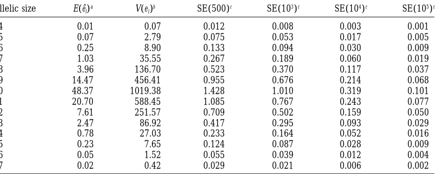
TABLE 1
Standard errors in estimating eiin a sample of 100 chromosomes
Allelic size E(eˆi)a V(ei)b SE(500)c SE(103)c SE(104)c SE(105)c
44 0.01 0.07 0.012 0.008 0.003 0.001
45 0.07 2.79 0.075 0.053 0.017 0.005
46 0.25 8.90 0.133 0.094 0.030 0.009
47 1.03 35.55 0.267 0.189 0.060 0.019
48 3.96 136.70 0.523 0.370 0.117 0.037
49 14.47 456.41 0.955 0.676 0.214 0.068
50 48.37 1019.38 1.428 1.010 0.319 0.101
51 20.70 588.45 1.085 0.767 0.243 0.077
52 7.61 251.57 0.709 0.502 0.159 0.050
53 2.47 86.92 0.417 0.295 0.093 0.029
54 0.78 27.03 0.233 0.164 0.052 0.016
55 0.23 7.65 0.124 0.087 0.028 0.009
56 0.05 1.52 0.055 0.039 0.012 0.004
57 0.02 0.42 0.029 0.021 0.006 0.002
The parameters used are A550, P50.1,a 50.6, andu 51.0. ae
iestimated from 200,000 independent samples. bThe estimated variance of e
i.
cThe standard error of an estimate with the number of samples given in parentheses.
as many other simulation experiments we performed eˆi5 1
M
o
jnij. (5)
suggest that for the purpose of identifying the vicinity of the MCS estimate, 500–1000 Monte Carlo samples is The estimator is unbiased with variance var(eˆi) 5 usually sufficient, and 10,000 Monte Carlo samples is var(ni)/M, where niis the number of alleles of size i in adequate for a fine-scale grid search to obtain the final
a single random sample of n chromosomes. It follows MCS estimate.
that estimation accuracy increases with the number M We define ti(n) 5 ei/n as the proportion of alleles of simulated samples. Therefore, the ability to simulate being size i and measure the closeness between {ti(n)} a large number of samples in a reasonable amount of for two different sample sizes by Euclidean distance, i.e., time is critical for the MCS estimator to be practical.
Coalescent algorithm is ideal for this purpose, and a d5
!
o
i
(ei/n2e9i/n9)2, sample of n alleles from a locus from a population
evolv-ing accordevolv-ing to a SMM with valueG 5(u, P,a, A) can
where e9i is the expected number of alleles i in a sample be simulated as follows:
of size n9. An interesting observation that we made in First, a genealogy of n sequences (alleles) is generated
our simulations is that values of {ti(n)} become steady using a coalescent algorithm (e.g., Hudson1991). For
rapidly even for a modest sample size. Table 2 shows the simulated genealogy, we have not only the
topologi-several examples of Euclidean distances between {ti(n)} cal relationships of these sequences, but also the
num-of different sample sizes. Note that the difference be-ber of mutations that occurred on each branch of the tween them when sample size is larger than 100 is ex-genealogy. Simulation of such a genealogy requires only
the value ofu. Second, assign a value to A, which is by
definition the allele at the root of the genealogy; then TABLE 2
determine the resulting allele of each mutation that
Estimated Euclidean distance between {ei/n}
occurred on the genealogy. Obviously the exercise re- of different sample sizes
quires knowing the allele type before a mutation and
can be accomplished by starting from the root and prog- Sample size
ressing toward the tips of the genealogy. In this process,
Sample size 25 50 100 200
the type of a new mutant allele is simulated according
to the distribution {pi}, which is completely specified by 50 0.0077
100 0.0101 0.0030
the values of P anda.
200 0.0129 0.0055 0.0031
Table 1 shows examples of the values of eˆiand their
400 0.0135 0.0062 0.0036 0.0013
standard errors for different numbers of Monte Carlo
samples. Note that the majority of estimates are reason- The ei for each sample size was estimated from 200,000
independently simulated samples. P50.1;a 50.5;u 51.0.
tremely small. This observation, although not too sur- P 5 0.01(0.01)0.10(0.05)0.9, and a 5 0.5(0.5)1.0, a total of 14,500 combinations of values of the three pa-prising from the viewpoint of coalescent process, is a
reward for our MCS method, because it means that one rameters. For each set of parameters, we generated 20,000 independent samples and obtained estimates of can convert with excellent accuracy the estimate eˆi for
a sample of size n to the corresponding estimate for a ei/n from (5). Note that we do not need to estimate ei/ n fora ,0.5 separately, because they can be obtained sample of size m by meˆi/n, saving considerable computer
cpu time when many samples are to be analyzed. from those fora .0.5 because of symmetry. Therefore,
we effectively obtained estimates of ei/n for 29,000 sets of parameters. These estimates were stored in a database
APPLICATIONS
and can be retrieved easily.
For each of the 63 samples, we performed a grid Since the discovery of highly polymorphic CA-repeat
loci (LittandLuty1989;WeberandMay1989), many search over all the parameter sets to obtain a MCS esti-mate ofG. In other words, for each of 29,000 parameter samples of such loci from human populations have been
reported (e.g.,Kaminoet al. 1993;Bowcocket al. 1994; sets, we computed thex2value, updated the minimum x2value and corresponding parameter values, and ob-Di Rienzoet al. 1994;Dekaet al. 1995). The samples of
Dekaet al. (1995) are particularly useful for population tained the MCS estimate after all the parameter sets had been examined. This fine-scale grid search still requires study because their sample sizes are relatively large and
the populations sampled are anthropologically well de- nontrivial computer cpu time but is quite manageable. The estimation results are given in Table 3.
fined. We thus use their data to illustrate our method
and to examine several issues about the evolution of Note that 26 of the 63 samples show contraction
(a ,0.5) in allele sizes and 37 show expansion (a . microsatellite loci. Eight CA-repeat loci in nine different
populations, the Samoan (SA), Dogrib Indian (DG), 0.5) in allele sizes (Table 3). This suggests that there is a slight bias of mutations toward expansion. Table 3 Pehuenche Indians (PH), New Guineans (NG), Kachari
(KA), German (GR), CEPH (CP), Sokoto (SO), and also suggests that most of the loci evolve in a multi-stepwise fashion. We divided samples into two groups, Chimpanzee (CH), were reported inDekaet al. (1995),
but we shall exclude the locus D13S137 from our analy- one showing allele size contraction and the other expan-sion; we then found that P values of the latter group sis because there are many single nucleotide insertions/
deletions within the repeat motifs at the locus. For the are considerably larger than those of the former group, which means that size change during expansion is likely remaining seven loci, we also exclude all the alleles
that are results of single nucleotide insertion/deletion greater than that during contraction. This result implies that if the probability a of expanding allele size by a because the mechanisms for changing allele size and
for insertion/deletion are likely different. The allele mutation is the same as or even slightly smaller than the probability of contracting allele size, the alleles in sizes and their frequencies at these loci are given in the
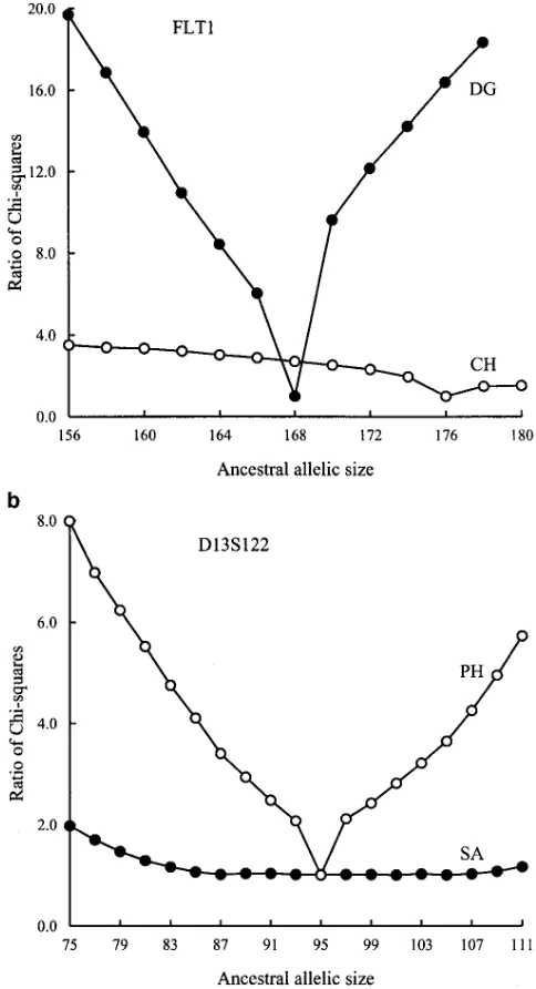
appendix ofDekaet al. (1995). Figure 3 shows the allele a population will still tend to increase in size. Because Table 3 shows thatain the majority of samples is larger frequencies at the loci FLT1 and D13S122. Because
polymerase chain reaction (PCR) was used for amplifi- than1⁄
2, there is a tendency, stronger than that suggested byaalone, that most loci are expanding in allele size. cation and the distances between the upstream primer
sequences and the first CA-repeat were unknown for Rubinszteinet al. (1995) compared allele sizes of 42 microsatellite loci in several primate species and found these loci, the resulting alleles were given in terms of
sequence length from the primer sequences, instead of that alleles in humans are generally longer than in other primates. They argued that microsatellite loci can evolve copy numbers. This does not pose difficulty in our
analy-sis because the mutation model (1) is only dependent directionally and at different rates in closely related species. Our estimates of the ancestral allele sizes in on the relative number|i2j|of copy numbers, which
are available from the samples. However, the estimated human populations and in chimpanzees also show a slight bias toward longer alleles in humans than in chim-ancestral allele A at each locus will have to be given in
terms of sequence length from the primer sequence. panzees, because the ancestral alleles of humans in five (FLT1, D13S118, D13S71, D13S122, and D13S124) of Our task of estimation appears to be challenging at
first glance because there are 63 samples to be analyzed, the seven microsatellite loci are longer than those of chimpanzees. However, some of these differences may each requiring a considerable amount of computer cpu
time. The observation we made earlier that the propor- be due to ascertainment bias, and analyses of more loci are needed to resolve this issue.
tion of alleles of a given size is rather insensitive to
sample size is of great help. Instead of generating a Weber and Wong (1993) studied 28 microsatellite loci in human chromosome 19 and a total of 20,000 large number of samples for estimating ei for each of
the 63 samples, we choose to obtain good estimates of parent-offspring allele pairs. They found that 78% of the 24 size changes in vivo were either gain or loss of ei/n for a sample of 100 chromosomes only and
Figure 3.—Allele
fre-quencies at loci FLT1 and D13S122.
in vivo and in vitro are considered, there is a strong bias may be occurring both in vitro and in vivo, and when both in vitro and in vivo mutations found in their tendency toward gains over losses in repeat units. Our
analysis in general agrees with their observations. In vivo study are considered, the mutation pattern would agree well with larger P values.
mutations as observed byWeberandWong(1993) do
not appear to suggest large P values. However, they do Letuijbe the value ofufor the ith population at the jth locus. If these loci are selectively neutral, then it not necessarily contradict our estimates: first, because
the number of mutations found in each locus examined would be reasonable to assume that the mutation rate at each locus is the same for different populations. in their study is simply too small to yield a reliable
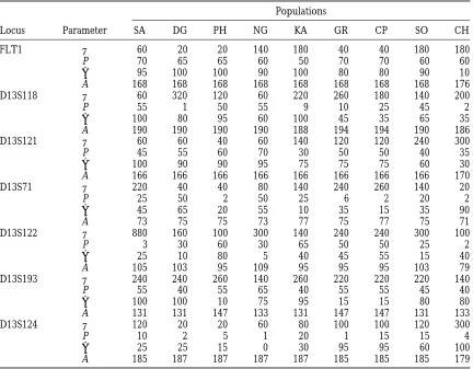
TABLE 3
Estimated values (3100) of parametersu, P,a, and A
Populations
Locus Parameter SA DG PH NG KA GR CP SO CH
FLT1 u 60 20 20 140 180 40 40 180 180
P 70 65 65 60 50 70 70 60 60
a 95 100 100 90 100 80 80 90 10
A 168 168 168 168 168 168 168 168 176
D13S118 u 60 320 120 60 220 260 180 140 200
P 55 1 50 55 9 10 25 45 2
a 100 80 95 60 100 45 35 65 35
A 190 190 190 190 188 194 194 190 186
D13S121 u 60 60 40 60 140 120 120 240 300
P 45 55 60 70 30 50 50 40 35
a 100 90 90 95 75 75 75 60 30
A 166 166 166 166 166 166 166 166 170
D13S71 u 220 40 40 80 140 240 260 140 20
P 25 50 2 50 25 6 2 20 2
a 45 65 20 55 10 35 15 35 90
A 73 75 75 73 77 75 77 75 71
D13S122 u 880 160 100 300 140 240 240 300 100
P 3 30 60 30 65 50 50 25 2
a 25 10 80 5 40 45 55 15 40
A 105 103 95 109 95 95 95 103 79
D13S193 u 240 240 260 140 260 220 220 220 140
P 55 40 55 65 40 55 55 45 40
a 100 100 10 75 95 15 15 80 80
A 131 131 147 133 131 147 147 131 133
D13S124 u 120 20 20 60 80 100 100 120 300
P 10 2 5 1 20 1 15 15 4
a 25 25 15 0 30 95 95 60 100
A 185 187 187 187 187 185 185 185 179
of the jth and j9th populations, respectively. That is, the the accuracy of simultaneous estimation of all four pa-rameters in a SMM model is undoubtedly more difficult, ratio ofus of two different populations is independent
of the locus studied. If estimates ofuare accurate, then but nevertheless of great importance for recommending a method. This is an area in which answers demand we should expect to see a consistent value of ratio of
us over different loci. The estimatedus in Table 3 show substantially more computer resource than estimation, and it deserves much effort in the future. Therefore, that this ratio for most pairs of populations is not very
consistent over loci. This suggests that the variance in we do not intend to provide all the answers here. In-stead, we will focus on discussing the accuracy in the
u estimate is likely to be large. The estimated us also
vary considerably among different populations for each estimation of ancestral allele A. Although estimates of the four parameters are interrelated, we observed that locus, but this is expected because of different effective
population sizes. A large variance in the estimation of values of the three parameters p,a, anduthat result in
x2 that is close to the minimum are also close to the
u is not unexpected because the estimate of u, [for
example, byWatterson’s (1975) estimator], from seg- set that results in minimum x2, while MCS estimates conditional on different ancestral alleles can differ sub-regating sites of DNA sequences that contain more
infor-mation aboututhan microsatellite data, is also accompa- stantially. This is not difficult to understand. For exam-ple, specifying a small ancestral allele size (relative to nied by a relatively large variance. Furthermore,Kimmel
andChakraborty(1996) showed that the variance of the sizes of alleles in a sample) will require large a and P (oru) to explain the observed allele frequencies, a variance estimator ofudoes not diminish with sample
size. while, on the other hand, specifying a large ancestral
allele size will result in a small estimated value for a. When we draw conclusions based on estimated values
of parameters, which are associated with variances, it is Our experience suggests that accuracy in the estimation of an ancestral allele is a good indicator of the overall important to have some measures of accuracy in the
estimates. Often the variance of an estimate of a single accuracy of estimation.
D13S122. It is interesting to note that estimated A 5 105 for the SA sample is not the most frequent allele in that sample. Table 3 shows that theuestimate from this sample is suspiciously large. Because Figure 3b shows that the estimate of A for this sample is rather uncertain, we expect that quite different sets of P, a, and u can result in x2 values close to the minimum. Indeed, when ancestral allele A is set to 85 the condi-tional minimum x2 value is equal to 154.59, which is less than 1% larger than the minimum x2 value, and the corresponding estimates of P,a, anduare 0.3, 1.0, and 4.2, respectively.
When the ancestral allele is reasonably certain, it makes sense to examine closely the estimation of other parameters. Take the locus D13S122, for example; allele size 95 appears to be the ancestral allele for the PH and GR samples (see Figure 3 and Table 4). Under the condition A595, we examined the minimumx2values for different values ofa, and results are given in Figure 5. For the PH sample, Figure 5 shows that it is very unlikely thata ,0.5 while for the GR sample,ashould not be substantially different from 0.5. These conclu-sions are reinforced by the allele frequencies in the two samples that are shown in Figure 3.
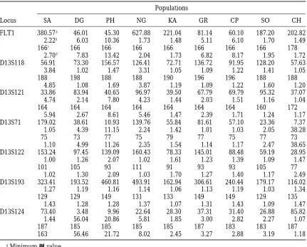
Another measure R2of accuracy is the ratio of thex2 value of the second best estimate of A to that of the best. The larger the ratio, the worse the fit for the second best A, and thus the better the estimate of A. Another useful measure Rmis the ratio of the meanx2values of the two neighboring sizes of A to that of A, which mea-sures the goodness of the A compared to its neighbors. Obviously we always have R2#Rm. These two measures are particularly convenient when there are many sam-ples to analyze, as in our situation. The values of R2and Rm, as well as the minimumx2value for the 63 samples, are given in Table 4.
Table 4 shows that 43 of the 63 samples result in R2. 1.20, and 30 result in R2.1.5. Although further study is required for proper interpretation of these R2 Figure4.—Examples of the ratio ofx2over the minimumx2.
values, it appears that other than the MCS estimate an increase of 20% or more in thex2value for an ancestral allele should be a reasonable indication that the estima-compare the minimum x2values conditional on
differ-tion is not totally out of line. ent ancestral allele sizes. One way to facilitate the
com-parison is a plot of x2values vs. various ancestral allele
sizes. A sharp decrease in the overall minimum value DISCUSSION
ofx2at allele A should suggest high accuracy of
estima-A strength of the MCS estimator developed in this tion. To allow comparison of the estimates for different
article is its ability to simultaneously estimate all the samples, we use the ratio of conditional minimumx2to
parameters of the SMM, including the ancestral allele, the overall minimumx2. Figure 3 shows two examples.
making better use of available information in a sample. Part a suggests that the estimate of A for the FLT1 locus
To date, mutation mechanisms for minisatellite and from population DG is accurate but the estimate from
microsatellite loci are not yet fully understood, and even population CH is uncertain. The allele frequencies in
less is known about the mode of mutations, i.e., whether Figure 3 concur with this analysis, because the frequency
it is symmetric or nonsymmetric, single-step or multi-of estimated A 5 168 in the DG sample is extremely
step. Although Kimmel et al. (1996) andKimmel and high, while the frequency of estimated A5176 in the
Chakraborty(1996) emphasized that allelic size vari-CH sample is only intermediate, although it is the
varia-TABLE 4
Some measures of quality in the estimates of ancestral allelic type
Populations
Locus SA DG PH NG KA GR CP SO CH
FLT1 380.57a 46.01 45.30 627.88 221.04 81.14 60.10 187.20 202.82 2.22b 6.03 10.36 1.73 1.48 5.11 6.10 1.70 1.49
166c 166 166 166 166 166 166 166 178
2.70d 7.83 13.42 2.04 1.73 6.82 8.17 1.95 1.72 D13S118 56.91 73.30 156.57 126.41 72.71 136.72 91.95 128.20 57.63 3.84 1.02 1.47 3.31 1.05 1.09 1.22 1.41 1.05
188 198 188 188 190 196 196 188 188
4.85 1.08 1.69 3.87 1.19 1.09 1.22 1.60 1.20 D13S121 33.86 83.94 40.65 96.97 39.50 67.79 69.79 95.32 37.07 4.74 2.14 7.80 4.23 1.44 2.03 1.51 1.16 1.04
164 164 164 164 164 164 164 160 172
5.94 2.67 8.61 5.46 1.47 2.39 1.71 1.24 1.17 D13S71 179.02 38.61 10.93 139.76 55.84 81.61 57.10 23.36 7.37 1.05 4.39 11.15 2.24 1.42 1.01 1.03 2.05 38.28
75 73 77 75 79 77 75 77 73
1.10 4.99 11.26 2.35 1.54 1.14 1.17 2.47 38.65 D13S122 153.24 97.45 139.09 160.43 78.33 145.01 88.48 59.19 28.95 1.00 1.26 2.07 1.02 1.61 1.23 1.39 1.09 1.47
101 105 93 111 91 93 93 105 77
1.02 1.30 2.09 1.03 1.70 1.27 1.40 1.17 2.49 D13S193 323.41 193.52 460.81 493.91 162.94 306.61 240.44 179.17 116.02 1.27 1.19 1.16 1.14 1.06 1.13 1.19 1.03 1.34
129 129 149 131 133 149 149 129 135
1.43 1.28 1.28 1.37 1.07 1.31 1.43 1.09 1.47 D13S124 73.40 3.48 9.96 22.64 28.30 37.31 31.40 26.88 85.82 1.44 56.04 20.86 5.81 1.85 3.00 2.82 2.27 1.07
187 185 185 185 185 187 183 183 187
163 56.46 21.72 8.02 2.45 3.27 2.88 3.19 1.18
aMinimumx2value. bValue of R
2.
cSecond best ancestral allelic type. dValue of R
m.
tion at repeat loci are not affected by asymmetry of allele subdivided populations. This strength should not be overlooked for two reasons. First, rapid accumulation size changes by mutations, their analyses reflect as well
the concept that knowledge of the distribution of size of population samples from microsatellite and mini-satellite loci provides excellent opportunities to exam-change by mutation is critical. Furthermore, the modes
of mutations are likely to differ from loci to loci. There- ine various mutation models, and, second, many natural populations, particularly human populations, are not fore, being able to estimate simultaneously all the
pa-rameters of a SMM has considerable advantages over panmictic. Proper statistical inferences should be based on more realistic population models, allowing for popu-methods for estimating a single parameter that assume
a mode of mutations, such as a symmetric single-step lation growth and subdivision. The expectation of alleles of a given size as estimated by Monte Carlo simulation mutation model, which may be grossly incorrect.
Another strength of our method is its flexibility. Al- provides great flexibility of the method, although it has the drawback of requiring more computer cpu time. though we only considered a mutation model with three
parameters and assumed a constant population size, it Note that methods for parameter estimation that rely on Monte Carlo samples to obtain some necessary quan-is not difficult to see that any combination of mutation
model and population genetics model can be analyzed tities were used inFu (1994).
The MCS estimator we developed is a generalized in a similar manner as long as alleles under these models
can be simulated. In particular, one can consider muta- least squares estimator and is often used in statistics for discrete distributions. Therefore, we expect our estima-tion models with constraints on allele size or mutaestima-tion
titative characters between populations or species. Genet. Res. 39:303–314.
Chakraborty, R.,andM. Nei,1997 Bottleneck effects on average
heterozygosity and genetic distance with the stepwise mutation model. Evolution 31: 347–356.
Deka, R., L. Jin, M. D. Shriver, L. M. Yu, S. DeCroo, J. Hundrieser
et al., 1995 Population genetics of dinucleotide (dC-dA)n ·(dG-dT)npolymorphism in world populations. Am. J. Hum. Genet. 56:461–474.
Di Rienzo, A., A. C. Peterson, J. C. Garza, A. M. Valdes, M. Statkin
et al., 1994 Mutational processes of simple-sequence repeat loci in human populations. Proc. Natl. Acad. Sci. USA 91: 3166–3170.
Ewens, W. J., 1972 The sampling theory of selectively neutral alleles.
Theor. Pop. Biol. 3: 87–112.
Fu, Y. X.,1994 Estimating effective population size or mutation rate
using the frequencies of mutations of various classes in a sample of DNA sequences. Genetics 138: 1375–1386.
Hudson, R. R.,1991 Gene genealogies and the coalescent process,
pp. 1–44 in Oxford Surveys in Evolutionary Biology, Vol. 7, edited byD. FutuymaandJ. Antonovics. Oxford University Press, New
York.
Jeffreys, A. J., V. Wilsonand S. L.Thein, 1985 Hypervariable
“minisatellite” regions in human DNA. Nature 314: 67–73.
Kamino, K., J. Nakura, K. Kihara, L. Ye, K. Naganoet al., 1993
Pop-ulation variation in dinucleotide repeat polymorphism at the D8S360 locus. Hum. Mol. Genet. 2: 1751.
Kimmell, M.,andR. Chakraborty,1996 Measure of variation at
DNA repeat loci under a general stepwise mutation model. Theor. Popul. Biol. 50: 345–367.
Kimmel, M., R. Chakraborty, D. N. Stivers andR. Deka,1996
Dynamics of repeat polymorphisms under a forward-backward mutation model: within- and between-population variability at microsatellite loci. Genetics 143: 549–555.
Kingman, J. F. C.,1982a The coalescent. Stochastic Process. Appl.
13:235–248.
Kingman, J. F. C.,1982b On the genealogy of large populations. J. Figure 5.—Minimum x2for different values ofa for PH
Appl. Probab. 19A: 27–43.
and GR samples at locus D13S122, conditional on ancestral Li, W. H.,1976 Distribution of nucleotide differences between two allele size being 95. randomly chosen cistrons in a subdivided population: the finite
island model. Theor. Popul. Biol. 10: 303–308.
Litt, M.,andJ. A. Luty,1989 A hypervariable microsatellite
re-vealed by in vitro amplification of a dinucleotide repeat within
coalescent algorithm, it is still a time-consuming method,
the cardiac muscle actin gene. Am. J. Hum. Genet. 44: 397–401.
which makes it hard to investigate the statistical
proper-Moran, P. A. P.,1975 Wandering distributions and the electropho-ties of the estimator. Nevertheless, the statistical proper- retic profile. Theor. Popul. Biol. 8: 318–330.
Nielsen, R.,1997. A likelihood approach to populations samples ties of the estimator will be worth studying in the future.
of microsatellite alleles. Genetics 146: 711–716.
There are a number of potential extensions to the
Ohta, T.,andM. Kimura,1973 A model of mutation appropriate method we proposed. We chose to obtain parameter to estimate the number of electrophoretically detectable alleles
in a finite population. Genet. Res. 22: 201–204.
estimates from allele frequencies, but the same
ap-Rubinsztein, D. C., W. Amos, J. Leggo, S. Goodburn, S. Jainet al., proach can be applied to a set of summary statistics, 1995 Microsatellite evolution—evidence for directionality and including various moments, number of alleles, heterozy- variation in rate between species. Nature Genet. 10: 337–343.
Shriver, M. D., L. Jin, R. ChakrabortyandE. Boerwinkle,1993 gosity, etc. It is also possible to incorporate variances
VNTR allele frequency distribution under the stepwise mutation
and covariances of allele frequencies into an estimator, model: a computer simulation approach. Genetics 134: 983–993. although doing so will demand even more computer Stuart, A.,andJ. K. Ord,1991 Kendall’s Advanced Theory of Statistics,
Vol. II, Ed. 6. Oxford University Press, New York.
resource. Another potential extension is to use thex2
Tautz, D.,1993 Notes on the definition and nomenclature of tan-statistics for testing hypotheses, such as the hypothesis demly repetitive DNA sequence, pp. 21–28 in DNA Fingerprinting: that mutations follow a single-step SMM, but hypothesis State of the Science, edited byS. D. J. Pena, R. Chakraborty, J. T.
EppenandA. J. Jeffreys. testing is likely to be more effective using
likelihood-Valdes, A. M., M. SlatkinandN. B. Freimer,1993 Allele
frequen-based approaches such as the method by Nielson
cies at microsatellite loci: the stepwise mutation model revisited.
(1997). Genetics 133: 737–749.
Watterson, G. A.,1975 On the number of segregation sites. Theor.
This work was supported in part by National Institutes of Health Popul. Biol. 7: 256–276.
grant R29 GM-50428 (Y.-X.F.) and GM58545 (R.C.). Weber, J. L.,andP. E. May,1989 Abundant class of human DNA
polymorphisms which can be typed using the polymerase chain reaction. Am. J. Hum. Genet. 44: 388–396.
Weber, J. L.,andC. Wong,1993 Mutation of human short tandem LITERATURE CITED repeats. Hum. Mol. Genet. 2: 1123–1128.
Weir, B. S., A. H. D. BrownandD. R. Marshall,1976 Testing Bowcock, A. M., A. Ruiz-Linares, J. Tomfohrde, E. Minch, J. R.
for selective neutrality of electrophoretically detectable protein
Kiddet al., 1994 High resolution of human evolutionary trees
polymorphisms. Genetics 84: 639–659. with polymorphic microsatellites. Nature 368: 455–457.