Fast and Scalable Algorithm For Sequencing Problems with Private Information

Fast and Scalable Algorithm For

Sequencing Problems with Private

Information

by

Ha Nguyen

August 18, 2014

Contents

1 Introduction 3

1.1 Mechanism design . . . 3

1.2 Sequencing problem with private information . . . 4

1.3 Research objective . . . 4

1.4 Research method . . . 5

1.5 Outline . . . 5

2 Background information and related literature 6 3 Mechanism design setting 10 3.1 Job-agents . . . 10

3.2 Private information . . . 10

3.3 Direct revelation mechanism . . . 10

3.4 Bayes-Nash incentive compatibility . . . 11

3.5 Individual rationality . . . 13

4 Problem formulation 15 5 Preliminaries 18 5.1 The type graph . . . 18

5.2 Virtual weights . . . 22

6 Answer to the sub-questions 27 6.1 Sub-question (I-2) Find and select the shortest paths in the two di-mensional setting . . . 27

6.2 Sub-question (I-1) Graph theoretic approach and optimal-IIA mechanism 31 6.3 Sub-question (II-1) Quality test . . . 35

7 AlgorithmF&E 42

8 Results and discussion 46

8.1 Description of instances . . . 46

8.2 Experiments for small scale instances . . . 48

8.3 Experiments for large scale instances . . . 59

8.4 Huge instances . . . 66

9 Conclusion 69 10 Appendix 71 10.1 Example 3: job’s data . . . 71

to maximize their own payoffs within the rules of the selling procedure, the seller will maximize his expected revenue over all such selling procedures.

The study of mechanism design looks at such issues. A mechanism designer needs to design a mechanism (a selling procedure in the above example) where strategic agents can interact. The interactions of agents result in an outcome. While there are several possible ways to design the rules of the mechanism, the designer has a par-ticular objective in mind. Depending on the objective, the mechanism needs to be designed in a manner such that when strategic agents interact, the resulting outcome gives the desired objective, where the resulting outcome is an equilibrium of the game amongst the agents, that is induced by the mechanism.

1.2

Sequencing problem with private information

Back to our study, the setting comprises a single server who can handle one job at a time, and job-agents j∈J ={1, . . . ,n}that compete for being processed. No job can be interrupted once started, and each job j is characterized by its processing time p_j

and weightw_j. The weightw_j represents job j’s disutility for waiting one unit of time. In addition, we assume that the service provider compensates jobs for waiting, while the job data are private and known to the job-agents themselves. The probability distributions of the private job data, however, are assumed to be publicly known. The problem is introduced in more detail in Chapter 2. This problem is an abstraction of economic situations where clients queue for a single scarce resource, for example, a specialized operation theater, while the information on the urgency and duration to treat each client is private, yet known probabilistically[1]. A concrete example for the latter are waiting lists for medical treatments in the Netherlands (Kenis 2006)[13].

1.3

Research objective

1.4

Research method

The one-dimensional case, where the processing times of jobs are publicly known and the weights are the only private information, is solved, in polynomial time, by a version of Smith’s rule[2, 6]. Smith’s rule is explained at the end of Chapter 2. It also has been shown that when both waiting cost and processing times are private, optimal mechanisms generally do not satisfy an independence condition known as IIA, and that a closed form for optimal mechanisms is generally not conceivable[2, 6].Though, it is known that optimal mechanisms can be computed in polynomial time if the scheduling rule is allowed to be randomized[1].

We here aim at constructing an algorithm, that computes mechanisms fast. More pre-cisely, we want that in reasonable computation times the algorithm produces mecha-nisms of good quality. To do that, we use the insight gained from the related literature. The quality of the algorithm, i.e. the quality of the output mechanisms and the speed of the algorithm are then proven through empirical research. The algorithm will be called AlgorithmF&E, which stands for fast and effective.

1.5

Outline

of optimal expected total payment. So together with inequality (2.1) we have

Expected total payments optimal randomized mechanism ≤ Expected total payments optimal deterministic mechanism

≤ Expected total payments optimal deterministic, IIA mechanism (2.2)

and there exist instances where the above inequalities are strict.

Note that in the single dimensional setting the two inequalities above are equalities instead. For the two-dimensional case, the complexity to find an optimal deterministic mechanism, with or without IIA-condition, remains open, and it is not even clear if the decision problem is contained in NP.

As mentioned earlier, we explain hereSmith’s rulebecause we make use of it a lot in this thesis. Suppose that 1 machine has to processnjobs j∈J. Each job jhas positive processing time p_j and weight w_j, these information are publicly known. Figure 2.1 is an example of a schedule for 3 jobs, whereS_j is the waiting/starting time of job j.

Figure 2.1:Example of a schedule for 3 jobs on 1 machine

We want to schedule the jobs so that the sum of the weighted starting times,P_jw_jS_j

is minimized. Smith’s rule schedules the jobs in the order of non-increasing ratios

w_j/p_j. That Smith’s rule leads to an optimal schedule can be shown by a very simple interchange argument as follows.

We first prove that having non-increasing ratios is a necessary condition for a schedule to be optimal. Let f be a schedule in which the jobs are not in ratio order. Then, in

f, there is a jobγthat immediately precedes a job jand yet w_γ/p_γ<w_j/p_j. If jobγ starts at timeS_γ, then job jstarts at timeS_γ+P_γ. If we interchange these two jobs, this affects only their starting times, not those of other jobs. The result is a strict decrease in total cost, by

”

w_γS_γ+w_j(S_γ+P_γ)—₋”w_jS_γ+w_γ(S_γ+P_j)— = w_jP_γ−w_γP_j

= P_γP_j

‚

w_j

p_j − w_γ

P_γ

Π>0

a schedule in which the jobs are in ratio order and let f∗ be an optimal schedule. If

f 6= f∗ then in f∗ there is a job γ immediately preceding a job j, where j precedes

γin f. But then w_j/p_{j ≥}w_γ/p_γ (because in f the jobs are processed in the order of non- increasing ratios) andw_γ/p_γ≥w_j/p_j (by the first part of this proof and because

f∗ is optimal) and, therefore, w_γ/p_γ = w_j/p_j. Interchanging the order of job γ and

2. a payment scheme π.

After job-agents report their types t = (t1, . . . ,tn), and depending on those reported

types, the allocation rule is nothing but a schedule f(t)that determines the order in which the jobs are executed. Note that f(t)is a non-preemptive scheduling, because no job can be interrupted once started. Next to the allocation rule, there is a vector of paymentsπ(t) that assigns a payment to every job-agent in order to compensate them for their waiting.

In other words, for each type profile t:= (t₁, . . . ,t_n)∈T :=T₁×. . .T_n, the payment scheme is the vectorπ(t) = (π1(t), . . . ,πn(t)), whereπj(t)is the amount paid to job jand the allocation rule f is represented by a permutation of the set{1, . . . ,n_}. Such allocation rule representation is illustrated in the next example.

Example 1. Suppose we have an instance with 3 jobs. Job 1 has a type space

con-taining only one type, type(w₁,p₁) = (4, 1). For job 2, letW₂ ={2, 3}and P₂ ={1}, so job 2 has two types namely(w1₂,p2) = (2, 1)and(w22,p2) = (3, 1), and let the

cor-responding probabilities beϕ((w₂1,p₂)) =ϕ((w2₂,p₂)) =0.5. Job 3 has the type space

(w₃,p1₃) = (3, 2)and(w₃,p₃2) = (3, 3), withϕ((w₃,p₃1)) =0.8 andϕ((w₃,p2₃)) =0.2

So there are in total 1×2×2= 4 type profiles. As an example consider allocation rule f, assigning the following schedules to reported type profiles

[(4, 1),(2, 1),(3, 2)]→132 [(4, 1),(3, 1),(3, 2)]→123

[(4, 1),(2, 1),(3, 3)]→231 [(4, 1),(3, 1),(3, 3)]→312.

Consider the type profile [(4, 1),(2, 1),(3, 2)], agent 1 has no choice but reporting type(4, 1), if agent 2 reports type(2, 1)and agent 3 reports type(3, 2), then job 1 is processed first, job 3 secondly and job 2 lastly. For the other three type profiles, the representation of allocation rule f can be read in the same way.

3.4

Bayes-Nash incentive compatibility

We will be interested in the so-called Bayes-Nash setting. That is, given a mechanism

(f,π), in the Bayes-Nash model each job’s goal is to maximize its expected utility. Thus we next discuss the computation of the expected utilities.

3.4.1

Expected utility

weakly dominant strategy in expectation, so for every job j and every two types ti_j =

(wi_j,pi_j), tk_j = (wk_j,pk_j)∈T_j:

Eu_j(ti_j,ti_j) ≥ Eu_j(tk_j,ti_j)

⇔Eπ_j(ti_j)−wi_jES_j(f,ti_j) ≥ Eπ_j(tk_j)−w_jiES_j(f,tk_j) (3.2)

The expectation is taken under the assumption that all agents apart from j report truthfully. The inequality in (3.2) just expresses the Bayes-Nash equilibrium concept: under the assumption that no other job deviates from being truthful, job j’s expected utility is maximal when being truthful, too.

If for a given allocation rule f there exists a payment scheme π such that (f,π) is BIC, then f is called Bayes-Nash implementable. The payment scheme π is referred to as an incentive compatible payment scheme.

3.5

Individual rationality

Recall that next to Bayes-Nash incentive compatible, we require the mechanisms to be individually rational. Here, we explain what ‘individually rational’ means. Typically, there is an objective function that the designer wants to maximize or minimize. One common objective is to maximize the social welfare (the sum of the agents’ utilities), but there are many others. For example, the designer may wish to maximize revenue. However, there are certain constraints on what the designer can do. For example, it would not be reasonable for the designer to specify that a losing bidder in an auction should pay a large amount of money: if so, the bidder would simply not participate in the auction. To prevent such scenario, individual rationality (IR) constraints are used. IR constraints sometimes known as ‘voluntary participation’ constraints, which follows from the idea that an agent is often not forced to participate but can decide whether or not to participate. Essentially, individual rationality places constraints on the level of expected utility that an agent receives from participation.

So next to Bayes-Nash incentive compatibility, we impose individual rationality con-straints as well. Unlike in auctions, where participation is optional, we assume a priori that all jobs must be scheduled. Mathematically, individual rationality makes sure that the optimal mechanism design problem is bounded [6].

A mechanism (f,π) is (interim)individually rational (IR) if for every agent j and every typeti

j∈Tj

Eu(ti_j,ti_j) = Eπ_j(ti_j)₋wi_jES_j(f,ti_j)_≥0. (3.3)

Dummy type We introduce a dummy typetd_j for each job j, with probabilityϕ_j(td_j) =

0 , and making sure that the dummy type gives zero utility to the job, by defining

ES_j(f,td

j):=0 and Eπj(tdj) :=0 for all jobs j ∈J. Now, we impose the constraints

in (3.2) also for k = d, which then implies the inequalities in (3.3). Therefore, the dummy types together with the mentioned assumptions guarantee that individual ra-tionality is satisfied along with the incentive compatibility constraints.

For a job jhaving|W_j|=m_j and|P_j|=q_j, that is job jhas m_j weights andq_j process-ing times, it will also be convenient to identify the dummy type with (wmj+1

j ,p h j)for

So in order to exploit the graph theoretic approach, we need to implement an algorithm that finds and selects the shortest paths in the reduced type graphs efficiently.

3. (I-3) Analogous to sub-question (I-2), how do we compute the virtual weights for the two-dimensional instances?

For research question (II) we have the next sub-questions:

(II-1) How do we evaluate the quality of the (output) mechanisms?

(II-2) How do we evaluate the computation times of our algorithm (used to compute a mechanism for each instance)?

• arcs from type(wi_j,pk_j)to(wi_j,pk_j+1)for alli∈ {1, . . . ,mj}andk∈ {1, . . . ,q_j−1}.

A sketch of the reduced type graph is given in Figure (5.1).

Figure 5.1:Sketch of a reduced type graph

Therefore from this point forward, by ‘type graph’ we mean ‘reduced type graph’.

Minimal expected incentive compatible payments for implementable allocation rule f Depending on the scheduling rule f, the lengths of the arcs in the reduced type graph can be computed. After that , a lower bound for the expected payment

Eπ_j(wi_j,pk_j)for type(wi_j,pk_j)is found by taking the negative of the shortest path length from node(wi_j,pk_j)to dummy node(wd_j,p_j)in the type graph T_j(f). To verify this, let

P =h(wi j,p

k

j) =a0,a1, . . . ,am= (wdj,pj)

i

denote some directed path from (wi1

j ,p k1

j ) to the dummy node in the graph Tj(f)

for job j. Denote by`(P)its length. Let (f,π)be a Bayes-Nash incentive compatible mechanism. From inequality (5.2) we have

Eπ_j(a_i)_≤Eπ_j(a_i−1) +`_a

i−1ai for i=1, . . . ,m

Adding up themincentive constraints above yields

Eπ_j(wd_j,p_j)≤Eπ_j(wi_j,pk_j) +`(P)

By definition, we haveEπ_j(wd_j,p_j) =0, thus

0 ≤ Eπ_j(w_ji,pk_j) +`(P)

Recall that for any implementable allocation rule f, T_j(f) has no negative length directed cycle. Consequently, shortest paths exist for all nodes in the graph. In light of inequality (5.4), the next lemma has been proven

Lemma 2. [2, 6]For any implementable allocation rule f , the payment scheme defined by

• πj(tdj) =πj(w mj+1

j ,pj) =0and

• for i =1, . . . ,m_jand for k=1, . . . ,q_j, the paymentπf_j(wi_j,pk_j)equals the negative of shortest path’s length from (wi_j,pk_j) to the dummy node in the reduced type graph T_j(f)

is incentive compatible, (interim) individually rational and minimizes the expected total payment made to the jobs.

The lengths of the shortest paths depend on the expected starting times of the types and the expected starting times of the types depend on the public data of all jobs, i.e. the weights, the processing times, and the corresponding distributions of all jobs. However, the payments as defined in Lemma 2 are independent of the reported type profile. That is, job j receives one and the same payment when reporting type t_j

independent of what other agents report, so that π(t_j,t_−j) =π(t_j) = Eπ(t_j). Let us call this property‘independence of reported types’.

Because our algorithm draw ideas from the one-dimensional case, we briefly discuss the optimal payments for a given allocation rule f in one-dimensional setting. In the single dimensional case, the shortest paths in the type graphs T_j(f)are independent of the (implementable) allocation rule f. Due to the implementability of f, there are no negative cycles in the graph, so all shortest paths must be simple paths. Finding oneself in any node, one always takes the arcs that goes to the node on the right until the dummy node is reached, see Figure 5.2.

6 Answer to the sub-questions

In this chapter we answer the sub-questions that have been raised in Chapter 4. In order to exploit and embed the idea that leads to optimal mechanisms in the one-dimensional case, we first need to know how to find and select the shortest paths (Sub-question (I-2)), as well as how to compute the virtual weights (Sub-question (I-3)) for instances in the two-dimensional setting. Sub-question (I-3) was already answered in Section 5.2. Therefore, we here discuss Sub-question (I-2) first.

6.1

Sub-question (I-2)

Find and select the shortest

paths in the two dimensional setting

6.1.1

Finding the shortest paths

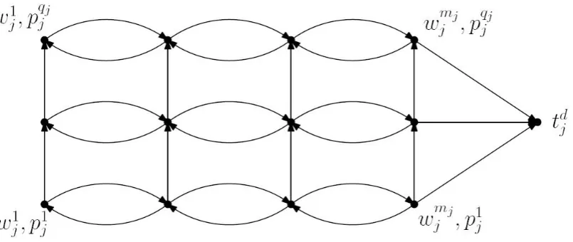
Ignoring the dummy node, the reduced type graph in the two dimensional setting looks like a grid, see Figure 6.1. Let(r,c)denotes the position of the node on row r

and columnc. So the types with highest processing time are lying in row 1, the types with second largest processing time are lying in row 2, etc.

Figure 6.1:Sketch of a reduced type graph

The only vertical arcs are those that go from row r to row r−1, with r =2, . . . ,q_j. Looking for shortest paths from a node in rowr, we only have to consider the part of the type graph that consists of row 1 to rowr. To take advantage of this property, we use dynamic programming for our shortest paths problem.

dummy node. Beginning with row 1 all shortest paths has the next form: starting in a node, one always takes the arc to the right until the dummy node is reached, just as in the single dimensional setting. For each node on row 1, the corresponding shortest path and its length are saved. Now consider a start node at position (2,c), to go to the dummy node one can either take

• the path that passes through only nodes in row 2 as in Figure 6.2

Figure 6.2

• or a path P that also passes through nodes in row 1, see Figure 6.3. Let (1,c0)

be the first node in row 1 that P enters and let divide P into two parts P₁ and

P₂, withP₁the path segment from(2,c)to(1,c0)and P₂the path segment from

(1,c0)to the dummy node. We want the length of P to be as small as possible, clearly P₂ should coincide with the shortest path from (1,c0) to the dummy node, which has been saved earlier. Obviously, shortest paths contain no cycle, i.e. they are simple paths. Because there is only one simple path from (2,c)to

(1,c0), this path must be taken to be P₁. So the length of P can be computed as the sum of`(P<sub>1</sub>)and`(P₂).

Figure 6.3

Note thatc0∈ {1, . . . ,mj}so there arem_jsuch pathsP, that should be examined.

then saved. Obviously, the process should be executed for all c = 1, . . . ,m_j and re-peated for all r =3, . . . ,q_j. With a start node, lying in row r, length of the path that passes through only nodes in row r and lengths of paths that also passes through nodes in row r−1 are being compared. The computation time for each type graph

T_j(f)has orderO(|W_j|.|Pj|2_).

6.1.2

Selecting the shortest paths

In the single dimensional case, from each node there is only one shortest path to the dummy node . This does not hold for the two-dimensional case, there can be more than one shortest paths from a node to the dummy node. The question is how should we deal with more shortest paths from one node, which path should be chosen? Through an example we explain how the virtual weights are computed when there are several shortest paths with the same start node. Consider the type graph in Figure 6.4, to keep a clear overview only arcs from the shortest paths betweena₀ anda₁₀are displayed.

Figure 6.4:Several shortest paths from node a₀ to dummy nodea₁₀

As can be seen, there are 5 shortest paths, namely

• P₁= [a₀,a₇,a₁₀],

• P2= [a0,a1,a2,a3,a4,a5,a6,a10],

• P₃= [a₀,a₁,a₄,a₅,a₆,a₁₀],

• P4= [a0,a1,a2,a3,a4,a5,a8,a9,a10],

Step 3, After that, the shortest paths to the dummy node can be found as described in Section 6.1.1 and the virtual weights can be computed using one of the three proposed methods in Section 6.1.2.

Step 4, The expected payments to job j is then given by formula 5.7. The expected total payment can be computed either as the sum of the expected payments to all job

jor with formula 5.11.

Step 5, Next, schedule the jobs according to Smith’s rule based on the ironed virtual weights. Let call this scheduling f1. Clearly, f1 is implementable.

Step 6, Now, apply step 2 to 5 to allocation rule f₁, the allocation rule we then get is called f₂. Repeat the process for f₂, etc.

In the above description, a stopping criterion is missing. However in our actual imple-mentation we observe that after a finite number of iterations, saykiterations, we get allocation rule f_k, where the corresponding virtual weights are identical to the virtual weights of allocation rule f_m with m< k. The value of k depends on the instances, especially the maximum number of types a job has, with other words the size of the largest type graph. If the method, used in step 3 for computing the virtual weights, takes into account all shortest paths (method 2 or method 3) then after iterationkwe get into a cycle: f_k coincides with f_m, f_k+1 coincides with fm+1, . . ., fk+(k−m)coincides

with f_k, etc. To illustrate all that has been said, we give the next example.

Example 2. We have 3 jobs withW₁={7, 8, 28},P₁={8}andϕ₁((7, 8)) =0.11844,

ϕ1((8, 8)) =0.76385,ϕ1((28, 8)) =0.11771. In Figure 6.5, job 1’s data are shown.

Figure 6.5: Job 1’s data

(a)Job 2 (b)Job 3

Figure 6.6:Job’s data

Using Smith’s rule as initial allocation rule f0 we get Pmin(f0) =366.55 as expected

total payment. We get Pmin_(f

1) = 374.68 independent of which method 1, 2 or 3

from Section 6.1.2 is used to compute the virtual weights in step 3. Now if we replace

W2={10}byW2={27}, and if other data are unchanged, we havePmin(f0) =470.51

and Pmin_(f

1) =470.51 when method 1 is used, Pmin(f1) =471.05 when method 2 is

used, Pmin(f₁) =471.05 when method 3 is used. As can be seen, it does not matter very much which method we use, the resulted expected total payments are of the same orders of magnitude. From now on, we use method 3.

The expected total payments when using method 3 andW2={10}are

Pmin(f₀) =366.55 Pmin(f₁) =374.68

Pmin(f₂) =353.85 Pmin(f₃) =354.83

Pmin(f₄) =353.85 Pmin(f₅) =354.83 . . .

The virtual weights that determine f4 are identical to the virtual weights that

deter-mine f₂. So we enter the cycle at iteration four and we can let the algorithm stop there. The computation time of these four iterations is 0.14189 seconds. In view of the results, one should process the jobs according to allocation rule f2.

Recall the LP-model by Hoeksma and Uetz in Chapter 2, in view of inequality 2.2, we can see the expected total payment obtained by the LP-model as a lower bound. Thus we can compare the result from our own algorithm to the lower bound. The relative difference from these two values is an indication of the performance of our algorithm. Besides the LP-model, Hoeksma[1]has implemented an ILP-model that computes the optimal IIA solution for small instances. Using his ILP, we found that the expected total payment provided by the optimal IIA mechanism, equals 353.85.

Example 3. In this example, there are 3 jobs as well. Job 1 has 4 types, job 2 has 40 types and job 3 has 42 types, for details see Section 10.1 in the appendix. The expected total payments are then

Pmin(f0) =527.76 Pmin(f1) =601.31 Pmin(f₂) =641.14 Pmin(f₃) =790.8

Pmin(f₄) =759.06 Pmin(f₅) =790.8.

The instance in this example is bigger than that from Example 2, in total there are 86 types while in the previous example there are 11 types in total. The computation time is 1.8771 seconds, so the computation time is not a problem. However, the proposed algorithm does not work well in this case. As can be seen, Smith’s rule gives the best result. The cause of the poor performance is not the larger number of types. Independent of the number of jobs, from all examples that we have seen, where the type graphs are not bigger than a 2×3 grid, the proposed algorithm works very well:

• the number of iterations is always less than 10,

• the output of the algorithm is a sequence of mechanisms. We take the best mechanism in this sequence, let π∗ denotes the corresponding expected total payment. Further, let Obj(LP) be the expected total payment computed by the LP-model. Recall thatObj(LP)is an lower bound for the optimal expected total payment. The ratioπ∗/ Obj(LP)is less than 1.02 for all instances we have seen, that is the expected total payment found with the algorithm is just 2% more than the lower bound. So in some cases it might be the optimal mechanism that the algorithm has found.

The poor performance is actually related to the ironing process. To see why, consider the next type graph

corresponding to nodea₁ is greater than that of nodea₀, so all shortest paths passing the segments a0−a1−a4 cause the virtual weight of a1 to increase, as can be seen

from the computations in Section 5.2. This way the virtual weights ofa₁ can become larger than that of nodesa₂and a₃, an as a consequence ironing must be carried out.

Similarly, when there are many shortest paths that go througha4−a5−a7 the virtual

weights of nodea₅can be very small, even negative because the weight corresponding to nodea₄ is larger than that of a₅. The chance is great that the virtual weight ofa₆

is larger than the virtual weight ofa5. Again ironing is necessary.

The larger the type graph the more such scenarios happen. When ironing is carried out to a large extent, many types with the same processing time will get the same expected starting time assigned, independent of weight. This apparently does not make a good allocation rule.

About research question (I), hitherto, we can only say that mimicking the point-wise-minimizing-algorithm of the single dimensional case does not yield a solution that is close to the optimal-IIA mechanism, at least not for reasonably sized instances. For instances where job agents has many types, the proposed algorithm even gives worse result than Smith’s rule. What we have learned from this is, in the search for a good mechanism using graph theoretic approach, we should try to avoid ironing as much as possible.

6.3

Sub-question (II-1) Quality test

In the Chapter 7, we will formulate our own algorithm, called Algorithm F&E (fast and effective). In Algorithm F&E we still make use of the graph theoretic interpre-tation and the concept of virtual weights, where we take into account the potential unfavorable effect of ironing in the two-dimensional setting. We also use Smith’s rule as initial allocation rule. In order to check whether or not the corresponding expected total payment is a good result, we can compare it to the LP-result (or ILP-result for really small instances) just as we have done earlier in Examples 2 and 3 in the pre-vious section. However, when the total number of types becomes really large, more than 1000, then even the LP-model can not handle the problem. In that case, we use the improvement in relation to Smith’s rule as performance’s measure.

6.4

Sub-question (II-2) Speed test

There is another question to answer, namely ‘when can we say that Algorithm F&E

First observe that for a solution (a mechanism) it suffices to give the allocation rule only, because the corresponding payments can be computed using Lemma 2. The

control algorithmsare standard algorithms based on a solution representation that

equals to a list of all types of the jobs. In this list the types are arranged in the order of non-decreasing importance. We illustrate such a representation in the next example.

Example 4. Suppose we have an instance with 2 jobs. Job 1 has a type space

contain-ing two types: t₁1and t2₁. Job 2 has a type space containing two types:t₂1and t2₂. So in total there 4 types. As an example consider the solution that is represented by the list below

{t2₂,t₁1,t2₁,t₂1_}

if job 1 reports type t₁2 and job 2 reports type t2₂ then job 1 is processed first because the types were arranged in the order of non-decreasing importance. Thus the corre-sponding allocation rule, assigns the following schedules to reported type profiles

[t₁1,t1₂]→21 [t₁1,t₂2]→12

[t2₁,t₂1]_→21 [t2₁,t₂2]_→12.

Also note that the list{t2₂,t₁2,t1₁,t1_2}, where the order of type t1₁ and type t2₁ are differ-ent from the earlier list, leads to the same allocation rule. Thus there can be several (list) representations that represent the same allocation rule, therefore equivalently the same mechanism.

We implemented several of such control algorithms: Simple local search, Simulates annealing, Global search. In order to make fair comparisons, we use the next stopping criterion for all control algorithms: ‘stop when a expected total payment is found, that is less than or equal to the one we found with AlgorithmF&E’. So we can compare the computation times needed by the algorithms to find more or less the same result. It might happen that the control algorithms get stuck in a local minimum, that lies above the result of AlgorithmF&E. For very large instances, it also might happen that a control algorithm does not get stuck in a local minimum, but it is still busy (still finding better results) after a ridiculously long time, but the result is not as good as that of Algorithm F&E. For this reason, time limits are being set for the control algorithms( we set the time limits to be 120 seconds for all control algorithms and all instances).

the metals crystallize themselves. As the metal cools its new structure becomes fixed, consequently causing the metal to retain its newly obtained properties. Simulated annealing is analogous to this annealing process. We keep a temperature variable to simulate the heating process. We initially set it high and then allow it to slowly cool as the algorithm runs. While this temperature variable is high the algorithm will be allowed, with more frequency, to accept solutions that are worse than our current solution. This gives the algorithm the ability to jump out of any local optimum at the initial stage of the execution. As the temperature is reduced so is the chance of accepting worse solutions, therefore allowing the algorithm to gradually focus in on an area of the search space in which hopefully, a close to optimum solution can be found. This gradual cooling process is what makes the Simulated annealing algorithm remarkably effective at finding a close to optimum solution when dealing with large problems which contain numerous local optima.

Figure 6.7: Simulated annealing

To help better understand, consider Figure 6.7. Suppose the red dot represents our current solution. Using the Simpel local search as described in Section 6.4.1, we will stay in this solution. In this example we can clearly see that it is stuck in a local optimum. In the mechanism design problem (or in any other real world problems), we would not know how the search space looks. So unfortunately we would not be able to tell whether this solution is anywhere close to a global optimum. By occasionally accepting worse solutions, Simulated annealing helps us to jump out of local optima we might have otherwise got stuck in. In this example Simulated annealing may helps us pass through the local minima, corresponding to the green dots and reach a better solution, corresponding to the blue dot.

The implementation of Simulated annealing is for the most part the same as the implementation of the Simple local search algorithm. The only differences are

• and the content of step 4, where a potential new solution is accepted.

The cooling schedule is a non-increasing function T : N→ (0,∞), T(i)is called the

temperature at theith-iteration. The temperature in our implementation decrease per 100 iterations, each time it decreases by 5%.

Step 4 is modified as follows: schedule the jobs according to the numbers, assigned to the types.

• If the corresponding expected total payment Pmin(f_new)is less than or equal to the current value, update f_c and Pmin(f_c) =Pmin(f_new). Empty the blacklist and go to step 5.

• Otherwise, compute the difference ∆ = Pmin(f_new)−Pmin(f_c). With probability

ρ, see formula 6.2, accept the exchange, update f_c and Pmin(f_c) = Pmin(f_new). Empty the blacklist and go to step 5. With probability 1−ρreverse the exchange and add the corresponding pair of types in the blacklist. Go to step 5.

ρ=exp−∆/T, where T is the temperature at that moment. (6.2) It remains to determine the initial temperature.

• Schedule the jobs according to Smith’s rule. Compute the corresponding ex-pected total paymentPmin(f₀). Set current expected total payment to bePmin(f_c) = Pmin(f0).

• Carry out randomly 10 exchanges, recall thatτis the total number of types. For each exchange, compute the corresponding expected total payment Pmin(f_new)

and the difference ∆ =Pmin(f_new)−Pmin(f_c). After that, we have 10∆-values. These values do not differ very much from each others. This is not surprising because by exchanging the (consecutive) numbers of just one pair of types, the change in allocation rule is minimal. Due to the small differences, we choose for just 10 random exchanges. For the moment, suppose that there is at least a positive ∆. Initial temperature is chosen such that if after Smith’s rule, the exchange with the most positive ∆, say ∆∗, happens, we accept the exchange with probability 0.5 and reverse (reject) the exchange with probability 0.5. That is T(0) = ∆∗_/ln(2).

We have assumed above that there is at least a positive ∆. In all our experi-ments this was also the case but for the completeness, return an error message otherwise.

6.4.3

Global search

if we consider two mechanisms that are the outputs of two consecutive iterations, there will not be a big difference between these two mechanisms with respect to the expected total payments. Hence, if any strict improvement occurs after an iteration, it is small. The same arguments hold for the Simulated annealing algorithm. Further, swapping costs almost no computation time, most of the work is the computation of the effect of a swap, i.e. the computation of the expected total payment after two types swap places in the solution representation list. So the it may be advantageous to adjust the Simple local search algorithm as follows. We repeat the swapping pro-cedure several times within an iteration, to obtain a very different new (Bayes-Nash implementable) allocation rule. We do not care about the effect of individual swap but the net effect of all swaps. If all swaps together do not cause the current expected total payment to increase then we accept all the swaps at once. We call this adjusted version of Simple local search, Global search.

The implementation of the Global search algorithm is for the most part the same as the implementation of the Simple local search algorithm. The only differences are

• we leave out the blacklist, because the probability that the same group of swaps happen at different iterations is nil.

• step 3 is modified as follows: let τ denotes the total number of types, repeat

τ/2 times the process below.

Consider all pair of types that satisfy the next conditions

– the types get consecutive numbers assigned.

– the types are from different jobs or from the same job but having different processing time.

7 Algorithm

F&E

First of all, recall our initial idea discussed in Section 6.2 , where we start wit the allo-cation rule f0, which is based on Smith’s rule with respect to the original weightswj.

Then the incentive compatible, individually rational payment scheme πf0 that

mini-mizes the expected total payment, can be computed using the shortest paths in the type graphs T_j(f₀), j ∈ J. The virtual weights are also computed using these short-est paths. Next, we schedule the job according to Smith’s rule with respects to the ironed virtual weights, the corresponding allocation rule is f1. The arc’s lengths in

the type graphs T_j(f₁) are in general not the same as the arc’s lengths in the type graphs T_j(f₀). Therefore, shortest paths in T_j(f₁) are different from the ones found inT_j(f0). That the shortest paths change, cause the virtual weights to change too. So

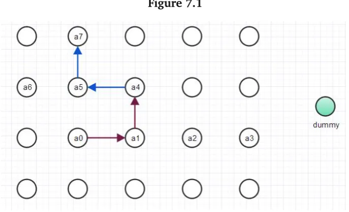
we get new allocation rule f₂, etc. This process results in a sequence of mechanisms with corresponding allocation rules f₀, f₁, f₂, . . . . From the implementation we ob-served that the sequence of output mechanisms consists of a finite number of different mechanisms, namely the algorithm eventually goes into a vicious cycle, i.e. it alter-nates between a few mechanisms. From all output mechanisms, we of course choose the best one. It turned out that the initial mechanism with allocation rule based on Smith’s rule with respect to the original weightsw_jis the best mechanism (amongst all mechanisms that have been output) most of the time, for reasonably seized instances. For these instances, it is pointless to run the algorithm, it takes time and the result by Smith’s rule is not improved. This poor performance can be attributed to the potential unfavorable effect of ironing (of the virtual weights) in the two-dimensional setting. Which in turn is caused by the fact that the shortest paths in the two-dimensional type graphs do not always go to the right until the dummy node is reached as in the one-dimensional setting, as stated in Section 6.2. For example, the path segment

a0−a1−a4−a5−a7 in Figure 7.1 does not has the configuration ‘only go to the right

until the dummy node’.

Figure 7.2: Type graphs by Smith’s rule

Figure 7.3:Type graphs by optimal rule

Comparing the optimal allocation rule to Smith’s rule, we see that the expected start-ing time of type (12, 6) of job 1, is decreased by 6 at the expense of the expected starting time of type(14, 6)of job 2. Due to the small probability of type(12, 6), the expected starting time of type(14, 6)is increased by just 0.6. This is the reason why the decline in expected payment to job 1 is much more than the increase in expected payment to job 2. If the probability of type(12, 6)was greater than or equal to 9/11 then the virtual weight of(12, 6)will be less than or equal to 14. That means optimal rule coincides with Smith’s rule.

It therefore seems beneficial to process types with small probability first, especially types that are lying on the ‘right-hand side’ of the type graphs because regularity still needs to be satisfied. Scheduling based on Smith’s rule with respect to the weights

f

8 Results and discussion

This chapter presents the results and discussion of Algorithm F&E described in the previous chapter. Chapter sections include first the description of test instances (Sec-tion 8.1), that are used for the valida(Sec-tion of Algorithm F&E. The experiments are divided into three classes based on the sizes of the instances, the class of small in-stances (Section 8.2), the class of large inin-stances (Section 8.3) and the class huge instances (Section 8.4).

Further, the validation is divided into two parts: the quality part and the speed part. That is for each instance we check whether or not the solution (mechanism) found is a good mechanism and whether or not AlgorithmF&Efound the solution fast?

For the quality validation, we compare the result ofF&Eto

• the ILP-result for really small instances.

• the LP-result for large instances. The instances are now too large for the ILP-model to handle, the ILP-model will not terminate in acceptable time.

• the result by Smith’s rule for huge instances. Theoretically, the LP-model can solve the problem in polynomial time. However the descriptions of the instances become so large such that so much memory is needed. As a result, the solver returns a memory error.

Other relevant information are: both the ILP[1] and LP-model[1]are implemented using programming language Python(version 3.2) and the solver Gurobi(version 5.2.6). AlgorithmF&Eis implemented in Matlab(version 2013b). All experiments were car-ried out on the system with

Operating system: Microsoft Windows XP.

Processor: Intel(R) Core(TM)2 Duo CPU T9300 @ 2.50GHz(2CPUs). Memory: 3072MB RAM.

For the speed validation, we compare the computation times of Algorithm F&E to the computation times of the three control algorithms described earlier in Section 6.4, namely Simple local search, Simulated annealing and Global search. These com-parisons of computation times are done for small and large instances. For the huge instances, we only report the computation times of AlgorithmF&Ebecause after the experiments with small and large instances, it can clearly be seen that all three control algorithms are no match for AlgorithmF&E.

8.1

Description of instances

1. experiments for small scale instances;

2. experiments for large scale instances;

3. experiments for huge instances.

For the first class of experiments we have:

• 20 instances, each with 5 jobs, each jobs can have at most 3 different weights and at most 3 different processing times.

• 20 instances, each with 10 jobs, each jobs can have at most 3 different weights and at most 3 different processing times.

For the second class of experiments we generate

• 20 instances, each with 5 jobs, each jobs can have at most 10 different weights and at most 10 different processing times.

• 20 instances, each with 10 jobs, each jobs can have at most 10 different weights and at most 10 different processing times.

• 20 instances, each with 20 jobs, each jobs can have at most 10 different weights and at most 10 different processing times.

Finally, we have for the huge instances

• 20 instances, each with 100 jobs, each jobs can have at most 10 different weights and at most 10 different processing times.

Recall that the type of a job is represented by t_j := (w_j,p_j) ∈ T_j :=W_j ×P_j, where

W_j :={w1_j, . . . ,wm_j j}with w1_j <. . .<wm_j j, and P_j ={p1_j, . . . ,pq_jj}with p1_j <. . . <pq_jj. We generate the types by generating setW_j and P_j as follows.

Let Wj denotes the cardinality of W_j and Pj denotes the cardinality of P_j. For the instances, where each jobs can have at most 3 different weights and at most 3 different processing times, Wj and Pj are random integers from the interval [1, 3]. For the remaining instances, where each jobs can have at most 10 different weights and at most 10 different processing times,Wj andPj are random integers from the interval

[1, 10].

ForW_j we generate a vector containing Wj unique integers selected randomly from

1 to 20 inclusive, then we sort these unique integers in the increasing order. Analo-gously, for P_j we generate a vector containing Pj unique integers selected randomly from 1 to 20 inclusive, then these unique integers are sorted in the increasing order.

Simple local search terminates after 120.02 seconds because the time limit of 120 seconds is exceeded. Considering the big differences in finish times of the local search and the other two control algorithms, it is highly likely that the expected total pay-ment of 3815.187 belongs to a local minimum. We then increase the time limit of 120 seconds to 240 seconds, and let the Simple local search continue from the last found solution of 3815.187. We see that the objective value does not change after the extra time and because of the small size of the instance, we conclude that 3815.187 is a local minimum.

In order to be able to compare, we use only instances where all three control al-gorithms manage to find a expected total payment that is less than or equal to the objective value of AlgorithmF&E, within the time limit of 120 seconds. Instances as in Example 6 will be discarded.

In Example 7 we give a typical small scale instance (used in this class of experiments) and the corresponding results.

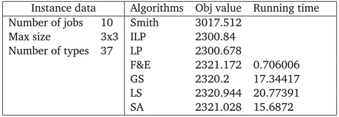
Table 8.2: Example 7

Instance data Algorithms Obj value Running time Number of jobs 10 Smith 3017.512

Max size 3x3 ILP 2300.84 Number of types 37 LP 2300.678

F&E 2321.172 0.706006 GS 2320.2 17.34417 LS 2320.944 20.77391 SA 2321.028 15.6872

Example 7. The objective value of the ILP-model is the expected total payment of

an optimal-IIA mechanism. The objective value of the LP-model is the expected to-tal payment of an optimal randomized mechanism. As stated earlier, the objective value of the LP-model is less than equal to that of the ILP-model. In this example, the mentioned inequality happens to be strict.

Because all mechanisms obtained by AlgorithmF&Eare deterministic and satisfy IIA condition, the ILP-model gives us tighter lower bound. In this class of experiments, we therefore use the results provided by the ILP-model.

8.2.1

Quality test

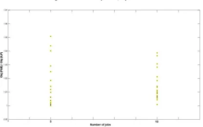
Recall that we have 20 instances, each with 5 jobs, each jobs can have at most 3 different weights and at most 3 different processing times. We arrange the instances in the order of increasing total number of types. In figure 8.1 the ratios computed by formula (8.1) are plotted against the total number of types. Take for example the point with coordinates(20, 1), this belongs to an instance whereP5_j=1|T_j|=20 and ratio 1 means AlgorithmF&E finds the optimal-IIA mechanism.

Figure 8.1:RatiosF&E/optimal IIA of 20 small scale instances, each with 5 jobs

So, for the instances with 11, 12 and 20 types Algorithm F&E finds the optimal-IIA mechanisms. For 8 other instances the ratios are less than 1.01. So for those instances the expected total payments by AlgorithmF&Eare not more than 1% above the corresponding optimal-IIA expected total payments. The instance with the highest ratio has in total 23 types and the ratio is 1.051, which is still a very good result because the expected total payments by AlgorithmF&Eis just 5.1% above the optimal-IIA .

Figure 8.2:RatioF&E/optimal IIA of 20 small scale instances, each with 10 jobs

For 10 instances (out of the 20 instances) the corresponding ratios are less than 1.01, so the expected total payments by Algorithm F&E are not more than 1% above the corresponding optimal-IIA expected total payments for half of the instances. The in-stance with the highest ratio has in total 38 types and the ratio is 1.038.

Figure 8.3:RatioObj(F&E)/optimal IIA

As can be seen, in the worst case, the payment given by AlgorithmF&E is about 5% higher than the optimal IIA payment. Approximately for 50% of the 40 instances, Al-gorithmF&Egives a payment that is at most 1% higher than the optimal IIA payment. In short, AlgorithmF&Egives solutions of excellent quality for small test instances.

8.2.2

Speed test

To check whether Algorithm F&E is a fast algorithm. We compare the computation times needed by the algorithms to find more or less the same result. The control algorithms stop at the moment a expected total payment is found that is less than or equal to the objective value of AlgorithmF&E. As in the quality test, we arrange the instances in the order of increasing total number of types.

For instances with 5 jobs:

• the computation times of Simple local search and Algorithm F&E are plotted against the total number of types in figure 8.4. The green squares represent the computation times of Simple local search, the red dots represent the compu-tatuon times of Algorithm F&E.

the times of Simulated annealing, the red dots represent the times of Algorithm

F&E.

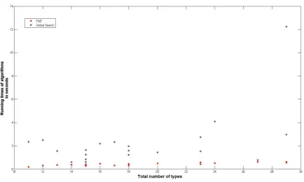
• the computation times of Global search and Algorithm F&E are plotted against the total number of types in figure 8.6. The black asterisks represent the times of Global search, the red dots represent the times of Algorithm F&E.

Figure 8.4:Computation times of Simple local search and F&E for instances with 5 jobs

Because there are 20 instances with 5 jobs, there are 20 red dots and 20 green squares in the plot. Take for example the points with coordinates(27, 0.6)and(27, 2.7). These two points belong to an instance that has in total 27 types, the computation time of AlgorithmF&E is 0.6 seconds. With a computation time of 2.7 seconds Simple local search finds a expected total payment that is less than or equal the expected total payment given by AlgorithmF&E.

Figure 8.5:Computation times of simulated annealing andF&E for instances with 5 jobs

Figure 8.6:Computation times of all algorithms for instances with 5 jobs

It can not be seen from the figures but using the test data, we have that the averaged computation time of Global search for 20 instances (each with 5 jobs) is 2.3 seconds. For the same 20 instances the averaged computation times of Simple local search and Simulated annealing are respectively 11.7 seconds and 8.3 seconds. Though, the averaged computation time of Global search is much smaller than the averaged computation times of the other two control algorithms, AlgorithmF&E defeat Global search at every instances. Moreover, the averaged computation time of AlgorithmF&E

is 0.4 seconds.

Figure 8.7:Computation times of the global search andF&Efor instances with 5 jobs

Figure 8.8:Computation times of the local search andF&Efor instances with 10 jobs

Figure 8.9: Computation times of simulated annealing and F&E for instances with 10 jobs

Figure 8.11:Computation times of all algorithms for instances with 10 jobs

re-• simulated annealing,

• global search,

• F&E.

the ratio of the algorithm’s objective value over the LP-model’s objective value. Be-cause all algorithms start from the Smith’s rule, the idea is to compare how much the result by Smith’s rule is improved by the control algorithms and by AlgorithmF&Ein the same amount of time.

For Simulated annealing, we will use the best found result and not the last found result. In example 8 we give a typical small scale instance (used in this class of exper-iments) and the corresponding results.

Table 8.3: Example 8

Instance data Algorithms Obj value Running time Number of jobs 20 Smith 25138.11

Max size 10x10 LP 19140.27

Number of types 445 F&E 21481.78 17.51188 GS 25109.35 18.66481 LS 25128.1 18.11799 SA 25137.14 17.94663

Example 8. In this example we see that the control algorithms hardly improve the

result of Smith’s rule with a time limit of 17.51188 seconds. As can be seen later in this section, Global search performs significantly better than the other two control algorithms. Even so AlgorithmF&Eoutshines all three control algorithms.

8.3.1

Quality test

Figure 8.12:Ratio expected total payment given by algorithms/expected total pay-ment given by the LP-model for instances with 5 jobs

Figure 8.13:Ratio expected total payment given by algorithms/expected total

Figure 8.14:Ratio expected total payment given by algorithms/expected total pay-ment given by the LP-model for instances with 20 jobs

For the quality test, we are only interested in the bottom most curves in the plots above, the curves that belong to AlgorithmF&E. For the moment, ignore other curves.

In the last two Figure 8.13 and Figure 8.14 we see that the two bottom most curves show the tendency to increase as the number of types increases. This suggest that the growth in total number of types may have a negative effect on the performance of AlgorithmF&E, with other words on the quality of the result of AlgorithmF&E.

Now, if we compare the tail of the curve in figure 8.12, more precisely the part of the curve that involve instances with the total number of types lying between 320 en 470, to the begin of the curve in figure 8.13, the part of the curve that involve instances with the total number of types lying between 330 en 550. The most ratios belonging to the begin of the curve in figure 8.13 are noticeably smaller than those belonging to the tail of the curve in figure 8.12, despite the fact that the instances in figure 8.13 have the same or large total number of types. Note that if instance A en B are both having the same total number of types, but instance A has fewer jobs, then on average instance A has more number of types per job. This seems to suggest that not only the total number of types affects negatively the performance of Algorithm F&E but also the number of type per job. However, recall that in one-dimensional setting, no matter how many types we have per jobs AlgorithmF&Ereturns the optimal IIA result. Thus it has also to do with how the type graphs look like, that is the configurations of the type graphs.

Figure 8.15:RatioOjb(F&E)/Obj(LP)

From Figure 8.15 we see that the ratio-range for large scale instances runs from 1.07 to 1.25. Recall that in the experiments for small scale instances we have a ratio-range from 1 to 1.05, see figure 8.3. This major shift in ratio-range can be explained by:

• the maximum size of the type graph was changed from 3×3 to 10×10. That means in the small instances, each job can have at most 9 types, now in the large instances, each job can have at most 100 types.

• a larger total number of types. The range of number of types was [11, 51] and for large instances the range is[65, 1006].

• a looser lower bounds by using the LP-model instead of the ILP-model.

Now consider also the other corresponding curves that belong to Smith’s rule, Sim-ple local search, Simulated annealing and Global search in Figure 8.12, Figure8.13 and Figure8.14. The curves of Smith’s rule are a little bit difficult to see because they largely overlap with the curves of Simple local search and Simulated annealing. These curves are far above the corresponding curves of AlgorithmF&E. That means the results given by Algorithm F&E are much better than the results given by other algorithms.

8.3.2

Speed test

For the speed test, we compare how much the result by Smith’s rule is improved by the control algorithms and AlgorithmF&Ein the same amount of time. Consider again figures 8.12, 8.13 and 8.14 now with all curves. Clearly, the improvements by Simple local search and Simulated annealing are negligible. Global search delivers better results, but still these improvements by Global search are insignificant compared with the improvements by AlgorithmF&E.

To give the readers some sense of the computation time of Algorithm F&E, we plot these times against the total number of types in figures for instances with 5 jobs, 10 jobs and 20 jobs respectively in Figure 8.16, Figure 8.17 and Figure 8.18.

Figure 8.16:Computation time of AlgorithmF&E for instances with 5 jobs

Figure 8.17: Computation time of AlgorithmF&Efor instances with 10 jobs

For test instances with up to 466 types in total, Algorithm F&E takes less than 30 seconds.

So for test instances with up to 1000 in total, AlgorithmF&Etakes less than 1 minute.

The computation times of AlgorithmF&Efor large instances are in the same order of magnitude as the computation times of the LP-model. Therefore we are satisfied with the computation times of AlgorithmF&Efor large instances.

8.4

Huge instances

As mentioned earlier, the LP-solver is not able to handle the huge instances, instances with 100 jobs. Hence for the huge instances we no longer have lower bounds for the expected total payments. We compute the ratios _{Obj(Smith’s rule)}Obj(F&E) in order to be able to say something about the quality of AlgorithmF&E.

Figure 8.19:RatioOjb(F&E)/Obj(Smith’s rule)at huge instances

Figure 8.20: RatioOjb(F&E)/Obj(Smith’s rule)at large instances with 20 jobs

As regards the speed of AlgorithmF&E, we plot the computation times of Algorithm

F&Eagainst the total number of types.

In summary, the results presented in this chapter show that AlgorithmF&E is a very good algorithm, in the sense that with AlgorithmF&Ewe have achieved the main goal of this thesis, namely, to find an algorithm that for each instance in small computation time, computes a mechanism that

• is Bayes-Nash incentive compatible and (interim) individually rational,

9 Conclusion

In the first part of the thesis, we explore the graph theoretic approach from related literature[2, 6]. It has been proved by Heydenreich et al. that

• the graph theoretic approach yields a closed form solution for the optimal mech-anism in the single dimensional case,

• in contrast to the one-dimensional case optimal mechanisms generally do not satisfy IIA condition in the two dimensional setting. As a result, the same graph theoretic approach, as used in the one dimensional setting, must fail to deter-mine an optimal mechanism for the scheduling problem.

This outcome gives rise to the question: ‘Can we then (approximately) compute de-terministic optimal-IIA mechanisms using the graph theoretic approach?’ which in turn leads to our initial implementation, explained in Section 6.2. In the initial im-plementation, the payments, the virtual weights are computed analogously to the one-dimensional setting. For each instance the algorithm outputs a finite sequence of mechanisms. The best mechanism is then selected as the solution.

Though it is a very fast algorithm, it turned out that for most of the reasonably sized instances, the algorithm resulted in solutions (mechanisms) where the corresponding allocation rules are just Smith’s rule with respect to the original weights. In spite of the fact that it is not a good algorithm, it does provide us new insight into the problem. That is, the ironing procedure as used in one-dimensional setting, may have potential unfavorable effects on the two-dimensional cases. It is not known yet whether there is a ‘better’ ironing procedure for the two-dimensional cases. The newly gained insight , together with intensive experimental research has led us to the alternative Algorithm

F&E. The validation ofF&Ewas divided into two parts: the quality validation and the speed validation. Both were done by applying AlgorithmF&E to 120 instances, with various seizes from small to huge.

As regards the quality, AlgorithmF&Eperformed really well for all tested instances:

• For small instances it found results that are at most 5% from the IIA-optimal results found by the ILP-model.

• For large instances it found results that are at most 25% from the lower bounds (for optimal results) found by the LP-model.

• For huge instances it improved the results by Smith’s rule by at least 12% and at most 23%.

Concerning the speed, it is impressive how fast Algorithm F&E is. Even though, we have constructed several control algorithms and we have made them as good as pos-sible, AlgorithmF&Eoutshines all three control algorithms at almost all instances. At really small instances, whereF&Edoes not ‘outshine’ the control algorithms, the com-putation times of AlgorithmF&E, are still noticeably smaller than those of the control algorithms. Moreover, AlgorithmF&Eare able to solve instances that are so huge that they are unmanageable for the LP-solver.

The results of this thesis point to several interesting directions for future work:

• In this thesis, an allocation rule (equivalently, a mechanism) is represented as a linear ordering of the types. By changing the ordering, we jump from mecha-nism to mechamecha-nism. But can we do this in a different way? Although the results presented in Chapter 8 have demonstrated the effectiveness of AlgorithmF&E, mechanisms found by Algorithm F&E always satisfy IIA-condition and optimal mechanisms in general do not satisfy IIA-condition. So maybe with another rep-resentation we are no longer limited to IIA-mechanisms.

• The work described in this thesis has been concerned with the mechanism de-sign problem for the sequencing problem with private information. For the prob-lem we have found a method that was shown to be fast and effective. Is it pos-sible to transfer ideas to other mechanism design problems?

10 Appendix

14 0.0280 0.0149 0.0116 0.0329 0.0249 0.0613 0.0084 0.0207 10 0.0203 0.0404 0.0397 0.0137 0.0082 0.0240 0.0154 0.0153 9 0.0150 0.0045 0.0262 0.0226 0.0184 0.0369 0.0317 0.0252 7 0.0420 0.2009 0.0027 0.0215 0.0090 0.0112 0.0129 0.0080 5 0.0012 0.0013 0.0032 0.0455 0.0211 0.0436 0.0024 0.0132

Table 10.2:Job 2

17 0.0075 0.0068 0.0567 0.0493 0.0217 0.0109 0.0378 14 0.0111 0.0069 0.0549 0.0356 0.0241 0.0424 0.0026 11 0.0070 0.0019 0.0622 0.0043 0.0143 0.0042 0.0462 8 0.0194 0.0141 0.0858 0.0398 0.0226 0.0025 0.0483 5 0.0198 0.0715 0.0155 0.0172 0.0284 0.0144 0.0345 2 0.0191 0.0092 0.0003 0.0010 0.0160 0.0106 0.0019

Table 10.3:Job 3

10.2

Determine the range for

α

Figure 10.1:10 jobs

The optimalα-value in Figure 10.1 is 0.3.

Figure 10.2:20 jobs

The optimalα-value in Figure 10.2 is 0.3.

Figure 10.3:30 jobs

Figure 10.4:40 jobs

The optimalα-value in Figure 10.4 is 0.3.

Figure 10.5:50 jobs

The optimalα-value in Figure 10.5 is 0.4.

Figure 10.6:100 jobs

Bibliography

[1] R. Hoeksma and M. Uetz. Two dimensional optimal mechanism design for a se-quencing problem. In: M. Goemans and J. Corréa, editors,Integer Programming and Combinatorial Optimization, volume 7801 ofLecture Notes in Computer Sci-ence, pages 242–253. Springer, 2013.

[2] B. Heydenreich, D. Mishra, R. Müller, and M. Uetz. Optimal Mechanisms for Single Machine Scheduling. In: C. Papadimitriou and S. Zhang, editors,Internet and Network Economics, volume 5385 of Lecture Notes in Computer Science, pages 414–425. Springer, 2008.

[3] Vladimír ˇCern`y. Thermodynamical approach to the traveling salesman problem: An efficient simulation algorithm. Journal of optimization theory and applica-tions,pages 41–51, 1985.

[4] Partha Dasgupta, Peter Hammond, and