Copyright1999 by the Genetics Society of America
Statistical Methods for Mapping Quantitative Trait Loci
From a Dense Set of Markers
Jose´e Dupuis* and David Siegmund
†*Genome Therapeutics Corporation, Waltham, Massachusetts 02453 and†Department of Statistics,
Stanford University, Stanford, California 94305 Manuscript received April 14, 1997 Accepted for publication September 21, 1998
ABSTRACT
Lander and Botstein introduced statistical methods for searching an entire genome for quantitative trait loci (QTL) in experimental organisms, with emphasis on a backcross design and QTL having only additive effects. We extend their results to intercross and other designs, and we compare the power of the resulting test as a function of the magnitude of the additive and dominance effects, the sample size and intermarker distances. We also compare three methods for constructing confidence regions for a QTL: likelihood regions, Bayesian credible sets, and support regions. We show that with an appropriate evaluation of the coverage probability a support region is approximately a confidence region, and we provide a theroretical explanation of the empirical observation that the size of the support region is proportional to the sample size, not the square root of the sample size, as one might expect from standard statistical theory.
R
ECENT advances in genetics have led to the identi- maize (Stuberet al. 1992); (iii) high blood pressure inrats (Jacob et al. 1991); and (iv) fatness and growth
fication of genes responsible for certain diseases
such as cystic fibrosis, Huntington’s disease, breast can- rate in pigs (Andersson et al. 1994). In their original
article, Lander and Botstein suggested statistical tests for cer, and others. Linkage analysis, which is especially
effective when the disease or trait of interest exhibits general designs, but provided guidelines for declaring statistical significance for the backcross design only. Mendelian inheritance, played an important role in the
identification of those genetic loci. When the disease is Paterson et al. (1991) used these guidelines for
in-tercross designs, but to avoid an increase in the false-complex in nature (incomplete penetrance, multiple
loci involved, etc.) or quantitative, finding the genetic positive error rate, they restricted themselves to a 1-d.f. statistic that ignored dominance effects. Churchill loci involved in the etiology of the trait can be more
difficult. In particular, in human studies, it is difficult andDoerge (1994) proposed use of the permutation distribution to define thresholds for all design types. to separate environmental and genetic effects. However,
with experimental organisms, studies can be designed This method has the advantage that it makes no assump-tions on the distribution of the phenotype. However, to provide a similar environment for all individuals, so
the thresholds depend on the observed data, so they that the variation in phenotypes can be attributed
need to be computed by Monte Carlo for each study; mainly to genetic factors; and breeding designs can
con-hence the method is less useful for analyzing and com-trol the nature of the differences in genotype. Studies of
paring different designs. experimental organisms can provide useful information
In this article we propose for intercross and other for agricultural purposes and/or contribute to our
un-designs simple approximations that can be used to com-derstanding of human disease via animal models.
More-pare different designs under various conditions or the over, it is now feasible to search the entire genome for
same design for different sample sizes or marker densi-a gene locus influencing densi-a trdensi-ait of interest. Stdensi-atisticdensi-al
ties. We also discuss and compare three methods for methods for mapping quantitative trait loci (QTL) from
constructing confidence intervals for a QTL. We assume experimental crosses using a dense set of markers were
throughout that markers are equally spaced, that there introduced byLanderandBotstein (1989).
Applica-are no missing data, and except where noted that recom-tions have involved (i) tomatoes (Patersonet al. 1991)
bination occurs without interference. While these are to identify loci influencing traits such as mass per fruit,
artificially simple assumptions, at the cost of some com-pH, and soluble solid concentration; (ii) grain yield in
plication they can all be weakened. Rough preliminary calculations suggest that the resulting picture would not change substantially unless the assumptions are radically Corresponding author: Jose´e Dupuis, Genome Therapeutics
Corpora-altered. The sections on QTL detection and confidence
tion, 100 Beaver St., Waltham, MA 02453-8443.
E-mail: [email protected] regions are independent and can be read in any order.
RESULTS stochastic model for the y’s. One can simply regard
the y’s as fixed numbers and the regression statistic The model and likelihood ratio statistics:The starting
essentially a weighted (by the y’s) sum of the x’s, to point for our considerations is a cross between two
which the central limit theorem applies under an as-strains that differ substantially in the quantitative trait
sumption that the empirical behavior of the y’s is about of interest. The parental lines can be “pure” breeding
what it would be if they were independent and identi-lines obtained through inbreeding or simply two
differ-cally distributed observations from a fixed distribution. ent strains of the same organism with widely differing
For backcross data, because xi(q)50 or 1, the additive
mean phenotype. A cross is obtained from the two
pa-and dominance effects cannot be estimated separately, rental lines, creating the first generation of offspring
and the model reduces to (generation F1). The F1 generation is then allowed to
mate together to produce the second generation (F2), yi5 m 1 a*xi(q)1 ei, (2)
the intercross. We assume that the genotypes of the
where the parametera* in (2) equalsa 1 dfrom the parental lines are completely different, so that at any
model (1). This is the model developed by Lander marker locus we can label alleles from the strain with
and Botstein (1989), which we review briefly here. the larger mean phenotype as A, and alleles from the
Treatment of the full model (1) is shown later in this other strain as B. At each locus, each individual of the
article. F2 generation will have zero, one, or two A alleles. A
If one observes the genotype of a marker at a putative backcross is generated by mating an individual of the
trait locus d, the maximum-log-likelihood ratio at d is F1generation to one from the parental line. If the
paren-given approximately by tal line with the smaller mean for the trait is used, the
offspring from the backcross will have zero or one A
alleles at any locus on their genome. 2 ln LR(d)≈2N ln(12 aˆ2
d/4sˆy2)≈
Naˆ2
d
4s2 e
, (3)
A standard model for quantitative traits (e.g.,
Kemp-thorne1957) in notation suitable for our purposes is where N is the number of typed individuals, aˆ
d is the
the following. Let yibe the phenotypic value of individ- maximum-likelihood estimate of the parameter a* 5
ual i, and let xij(d) be the number of A alleles at locus a 1 d, andsˆ2
y is the maximum-likelihood estimate of
d on the jth chromosome. The locus is identified by its the phenotypic variances2
y 5 s2e1 a*2/4. It is
impor-genetic distance d from one end of the chromosome. tant to note that boths2
y ands2edepend on the design
If there exists only one QTL on the jth chromosome and for a backcross differ from the corresponding quan-that influences the traits and its location is q, the pheno- tities for an intercross, although this difference is not
type can be modeled as reflected in the notation. Note also that (3) involves
natural logarithms; the marginal asymptotic distribution
yi5 m 1 axij(q)1 d1(x ij(q)51)1eij, (1)
of (3) at any unlinked locus isx2with 1 d.f. To convert
this and subsequent expressions to the LOD scale, one wherem,a,dare the phenotypic mean, additive effect,
and dominance effect, respectively, and 1Cequals 1 or can divide by 2 ln 10≈4.6. For the first approximation
in (3) we have replaced the empirical variance of {xi(d)},
0 according to whether the condition C is satisfied or
not. The eij’s are residual effects, which include both namely N21Ri[xi(d) 2 N21Rjxj(d)]2, by its asymptotic
value of1⁄
4; for the second we have approximated the
environmental effects and the genetic effects of QTL
on other chromosomes than the jth. As we will be consid- logarithm by the first term of its Taylor expansion and have replaced the estimatesˆyby the parametersethat
ering only a single chromosome at a time, we drop the
subscript j in what follows. We assume that xi(q) and ei it estimates under the hypothesis of no linkage on the
jth chromosome. Since the trait locus q is typically
un-are uncorrelated, which would be the case if there is
no epistasis and the environmental effect is uncorre- known, the log-likelihood ratio is maximized over all marker locations d and chromosomes j. At each marker, lated with the genetic effects. We also assume that the ei
are independent normally distributed random variables assumed to be a QTL, the log-likelihood ratio is com-puted exactly. Between markers,LanderandBotstein with mean 0 and variance s2
e. The residual variances2e
equals the sum of the environmental variance and the (1989) suggest the use of “interval mapping,” which consists of treating the unobserved marker information genetic variance for those QTL not on the jth
chromo-some. Without the normality assumption the regression- as missing data and using the EM algorithm (Dempster
et al. 1977) to evaluate the log-likelihood ratio at d based
like statistics given below are not exact
maximum-log-likelihood ratios, so it is possible that more powerful on the marker information at the flanking markers. A noniterative, regression-based alternative to the EM tests can be found. However, by virtue of the central
limit theorem the various approximations to signifi- algorithm was proposed byHaley andKnott(1992) and was shown to give equivalent results provided N is cance level, power, etc. will still be valid in large samples
even if the e’s are not normally distributed. In fact, for sufficiently large.
likelihood ratio is maximized over the entire genome, the QTL is located between markers, it is necessary to analyze the (correlated) process at the two flanking it is unclear whether the conventional threshold of
LOD53.0 [equivalently 2 ln LR(d).13.8] to declare markers. The more complex approximation, which re-quires a one-dimensional numerical integration, can be statistical significance is appropriate in the present
con-text. To address this issue,LanderandBotstein(1989) found inDupuis(1994). The noncentrality parameter at a flanking marker at distanceD1from the QTL is
proposed the approximation of N1/2a
dl/2se[cf. (3)] by
an Ornstein-Uhlenbeck process. This can be justified j
exp(2bD1), (6)
by the central limit theorem and a straightforward
calcu-lation of covariances. For the case of complete marker wherebandjare as defined above.
From (6) and (4) we see the importance of the param-information (continuous markers), they gave thresholds
depending on the length of the genome and the num- eterb, which equals 0.02 for backcross designs, but can assume a larger value for other designs (e.g., recombi-ber of chromosomes searched (cf. their Proposition 2).
For the case of a discrete set of markers evenly distrib- nant inbred designs). In (4),bmultiplies the length of the genome, so a larger value requires a larger threshold uted over the genome, they obtained thresholds from
a simulation study conducted under the assumption of to maintain a given false-positive error rate. From (6) we see that it also governs the rate at which the non-no interference.
For the case of equispaced markers along the ge- centrality parameter decays as a function of the distance from QTL to flanking marker. A large value ofbmeans nome,Feingoldet al. (1993) proposed an
approxima-tion, which agrees closely with the results from Lander a rapid falling off in power to detect the QTL as a function of that distance. On the other hand, it also and Botstein’s simulations. That approximation is
provides the possibility for more precise fine mapping
P {ma
kx 2 ln LR(kD).a} of the QTL location, because a largebleads to a sharper
delineation of the “peak” in the process 2 ln LR(d) that ≈12 exp{22C[1 2U(b)]
identifies the location of the QTL. We return to these 22bLbφ(b)n(b{2bD}1/2)}, (4)
issues below.
The preceding analysis is concerned with the likeli-where a5b2, L is the total length of the genome, C is
the number of chromosomes,b 52l,lbeing the rate hood ratio process observed at the discrete set of marker loci. To mitigate the problems indicated by (6) when of crossovers (l 51 if L is in Morgans andl 50.01 if
L is in centimorgans),Dis the distance between markers the QTL is in the center of a marker interval,Lander
and Botstein (1989) suggested the technique of in-in the same units as L, andF(x) andφ(x) are the
stan-dard normal cumulative and density function, respec- terval mapping, i.e., treating the unobserved intervals between marker loci as missing data and using the tively. The function n is a discreteness correction for
the distanceDbetween markers. The defining expres- EM algorithm to interpolate between the observed data points.Rebai et al. (1994, 1995) have used Rice’s
for-sion can be found inSiegmund(1985), p. 82. Often it
is adequate to approximate n(x) by exp(20.583x), mula for the expected number of upcrossings of a level by a piecewise smooth Gaussian process to give approxi-which is valid for x,z2, while for x.2 the first four
terms of the defining infinite series provide a reasonable mations for the false-positive rates when using interval mapping. The method is analytically tractable when one approximation. For the case of continuous markersD 5
0, son 51, and (4) is essentially the same as the approxi- assumes complete interference, i.e., the recombination probability and map distance in Morgans are equal. mation ofLanderandBotstein(1989).
For a backcross design with a QTL located exactly at Single chromosome simulations performed by these au-thors and our own whole genome simulations (data not a marker,Feingoldet al. (1993) gave as an
approxima-tion for the power shown) indicate that the approximation is very good
when the sample size is reasonably large and markers
P {ma
kx 2 ln LR(kD).a} are not too closely spaced. For dense markers (z1 cM) it
is conservative. A modification suitable for small samples ≈12 F(b2 j)
can be inferred fromJohnstoneandSiegmund(1989). 1 φ(b2 j)[2n/j 2 n2/(b1 j)2], (5)
An argument ofSiegmundandWorsley(1995) can be adapted to give a simple approximation for the power where a5 b2,j 5{N ln[11 (a 1 d)2/4s2
e]}1/2, andn 5
n(b{2bD}1/2), as defined previously. The parameterjis of an interval mapping test. Seeappendix a.
Intercrosses:Most previous theoretical analyses have the noncentrality parameter of (3) expressed in terms
of the parameters of the model (2). The first term in concentrated on backcrosses and consequently have ig-nored dominance effects.Patersonet al. (1991) used
(5) is the probability the process is above the threshold
at the QTL; the second is the probability that it is below the full model (1) to locate QTL in tomatoes in an intercross, and estimated the dominance effects. How-at the QTL but crosses the threshold How-at some nearby
2-d.f. statistic involving both additive and dominance effects.
Consider the likelihood ratio statistic to test the gen-eral hypothesis that a 5 d 5 0 vs. the alternative that a ? 0 or d ? 0. For intercross data the vectors with coordinates xi(d) and 1(xi(d)51)(i51, . . ., N ) are
asymp-totically orthogonal. Therefore, the approximations used to obtain (3) now yield for the log-likelihood ratio at the marker d
2 ln LR(d)≈2N ln
5
12 adl2/21 dˆ2
d/4
sˆ2
y
6
≈
31
N1/2aˆd21/2s e
2
2
1
1
N1/2dˆd2se
2
24
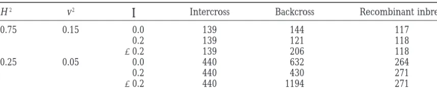
. (7)Figure1.—Thresholds for 350 simulated tomato genomes.
To define a significance level, we give an approximation under the hypothesis of no linkage to the distribution
of the maximum of (7) over all possible values of d. cally correct form of (9) involves similar complications,
Let although extensive numerical calculations show that
there is very little difference between the mathematically correct approximation and the more convenient one
Xd5
N1/2aˆ
d
21/2s e
and Yd5
N1/2dˆ
d
2se
. (8)
given above, which is based on replacing the two param-etersb1andb2associated with the two coordinate
pro-A straightforward application of the central limit
theo-cesses by their average value, (b11 b2)/2. In this spirit
rem and calculation of covariances shows that when
one can modify the approximation ofRebaiet al. (1995) a 5 d 5 0, for large N, Xd and Yd are approximately
to obtain a closed form approximation that is no more independent Ornstein-Uhlenbeck processes with mean
complicated than that obtained for a backcross and 0 and covariance functions e22l|t|and e24l|t|, respectively.
gives essentially the same numerical results as the more An approximation to the tail distribution of the
maxi-complicated, mathematically correct approximation. mum of (7) is provided by
To check the accuracy of (9) and our interval
map-P {ma
dx 2 ln LR(d)$ a} ping approximation, we simulated thresholds for the
log-likelihood ratio based on an intercross sample of ≈12exp
5
23
C 1 nb2L1
b11 b22
24
exp(2b2/2)
6
, (9)N5350 organisms with 12 chromosomes of total length 1200 cM (to approximate the tomato genome). The interval mapping step was performed using an approxi-where b1 5 2l, b2 5 4l, a 5 b2, and n 5 n(b{D(b1 1
b2)}1/2). As in the case of (4), this approximation does mation due toHaleyandKnott(1992), which is much
less computer intensive and gives results almost identical not take interval mapping into account. It is obtained
by a suitable modification ofWoodroofe’s (1976) argu- to the EM algorithm for large values of N. Results are shown in Figure 1.
ment. For an idealized tomato genome consisting of 12
chromosomes of length 100 cM each and a dense set Both approximations are very accurate. As predicted, the process with the interval mapping step requires a (D 5 0) of markers, the 0.05 false-positive threshold
obtained from (9) is a519.0 (LOD54.13), in compari- higher threshold for a given value of the Type-I error. For smaller N, somewhat different approximations yield-son with a514.6 (LOD53.17) for the backcross case.
Although smaller thresholds are required when the in- ing larger thresholds need to be used, since the given approximations do not take into account the variability termarker distance is greater, for an intercross the
con-ventional LOD 5 3 threshold would lead to a false- in the estimate of the variance,s2
y. However, when N is
large (at least 200), the approximations provide thresh-positive rate greater than 0.05 even for intermarker
distances of 25 cM. This stands in contrast to the case olds for the statistic and marker density actually used, which are more appropriate than the conventional LOD of a backcross, where the LOD53 threshold is
conserva-tive for intermarker distances down toz1 cM. 53.0. In mapping human traits,LanderandKruglyak
(1995) have argued that because the investigator is likely Rebaiet al. (1995) have given an approximation for
the false-positive error rate when interval mapping is to type more markers around promising loci, the thresh-old forD 50 should be used in all cases. If we use this used. This approximation involves an elliptic integral,
to be evaluated numerically, and so is more complicated threshold, it is not necessary to rationalize the choice ofD, which should otherwise be an average intermarker than the analogous backcross approximation, which can
mathemati-Figure 2.—Power to detect linkage for different map den-sities, gene locations, and thresholds. In a and b,D 55 cM whileD 520 cM in c and d. The trait locus is located at a marker in a and c and mid-markers in b and d. The pro-cess without interval mapping is represented byh; the pro-cess with interval mapping is represented by e (solid sym-bols for the theoretical approx-imation) and,(power for the higher threshold appropriate whenD 50).
ping on the false-positive error rate. But insistence on ping test. We also present the power of the interval this threshold would noticeably reduce the power of mapping test using the more stringent threshold
(as-the test, as is shown shortly. suming continuous markers) proposed byLanderand
For intercross data the noncentrality parameter for Kruglyak (1995). The power was investigated for a a QTL located at a marker locus isj 5{N ln[11(a2/ dominant model, sod 5 a, and j 5 4.12, 4.41, 4.75,
21 d2/4)/s2
e]}1/2. To attribute appropriate parts of the and 5.21, which correspond roughly to powers of 60,
total noncentrality to the two processes in (10), we let 70, 80, and 90% with a continuous map of markers. For j15 ja/(a21 d2/2)1/2,j25 jd/[2(a21 d2/2)]1/2. If the recessive (d 5 2a) models, the power would be exactly
QTL is located at a marker, the power is approximately the same. For the same noncentrality values and an additive model (d 50), it would be slightly larger. Power
P {ma
kx 2 ln LR(kD).a} under two map densities was estimated (D 520 and 5
≈12 F(b2 j)1 φ(b2 j) cM) and we used N5350 tomato genomes. Each power
simulation is based on 1000 replicates. The gain in 3
3
12j1 2b1/2n
j3/2 2
b1/2n2
j1/2(b1 j)
4
, (10) power from using interval mapping is small, on theorder of 2–4%, a result similar to that found byDarvasi
et al. (1993). The gains anticipated by Lander and
wheren 5 n(b{2bD}1/2),b 5(b
1j211 b2j22)/j2. For a QTL
Botstein(1986, 1989), who write of interval mapping between markers, one must as in the backcross case
as providing a “virtual marker” midway between the consider the joint distribution at flanking markers. For
actual markers, are overly optimistic. Their analysis is a marker at distanceD1from the QTL the noncentrality
parameters are marred by their comparison of interval mapping with
the marker process at only one of the flanking loci, j1exp(2b1D1) and j2exp(2b2D1). (11) where a more appropriate comparison would be with
the maximum of the process at the two flanking loci. Seeappendix afor an approximation for the power of
They also neglect the increase in threshold required to the interval mapping process.
maintain a given false-positive error rate for the interval Using simulations and the theoretical power
approxi-mapping process. The gain in power for interval map-mations above, we compare in Figure 2 the power of
gain is onlyz3–4%. Using the threshold for a continu- show that under the null hypothesis, X(d) is approxi-mately a Gaussian process with covariance function ous map when in fact a sparse map of markers is used
R(d)512 8⁄
3l|d|1o(|d|) as d→0. Therefore,
approx-greatly reduces the power (by as much as 20%).
imation (4) can be used withb 58⁄
3lto find an
appro-We have made similar computations with similar
re-priate threshold. sults for backcross designs.
Korolet al. (1995) have suggested the use of
corre-When the markers only process is used, the
theoreti-lated traits as a technique to improve the power of QTL cal power approximations are very good, so only the
mapping. If the number of traits is t, this would require simulated values have been included in Figure 2. The
a t dimensional version of (4) or a 2t dimensional ver-approximations are also good for interval mapping
ex-sion of (9) for the backcross or intercross design, respec-cept when the intermarker distance is 5 cM and the
tively. The appropriate k dimensional approximation QTL is midway between markers. In this case the power
(k5t or 2t) is given by
is underestimated byz5%. The reason is that the theo-retical approximation involves only the probability that
12 exp{2C[12Fk(b)]2 bL2(22k)/2
the process is above the threshold somewhere in the
interval containing the QTL and neglects the probabil- 3[G(k/2)]21bk
exp(2b2/2)}.
ity of detecting the QTL to be in a neighboring interval.
Here Fkis thex2distribution with k degrees of freedom,
This is not a problem when the intermarker interval is
Gdenotes the gamma function, andbwould be replaced large.
by (b11 b2)/2 for an intercross design. Corrections for
Other designs and a comparison of different designs:
discrete spacing of markers would be exactly as above. Many other designs can be handled by similar
approxi-We have used the theory developed above to compare mations. To evaluate an appropriate threshold, for the
the power of backcross, intercross, and recombinant markers only process it is only necessary to know the
inbred designs (obtained by recurrent sib mating). Let recombination parameter b (orb1 andb2), which de- s2
A,s2D,s2E denote the total additive, dominance, and
pends only on the design, not the mathematical model
environmental variances, respectively. Assuming that used for recombination. Although there is no general
environmental and genetic effects are uncorrelated and method to evaluate this parameter, it has been
calcu-there is no epistasis, we have the usual representation lated for many different designs. (Some values are given
of the phenotypic variance as s2
y 5 s2A1 sD2 1 s2E. Let
below.) For interval mapping one must know the
com-H25 (s2
A1 s2D)/s2y denote the wide sense heritability
plete covariance function, which depends on both the
in the intercross, and put r 5 d/21/2a. To reduce the
design and the model for recombination.
number of different special cases we assume that r is For instance, for recombinant inbred data, which
in-the same at all QTL; i.e., in-they all have in-the same relative volve the 1-d.f. statistic (3), one can use approximation
amount of dominance. If we let v2 be the heritability
(4) withb 50.04 for recombinants produced by selfing
attributable to the locus of interest, i.e., v2 5(a2/2 1
andb 50.08 for recombinants produced by recurrent
d2/4)/s2
y # H2, then the noncentrality parameters of
sib mating (as originally suggested by Lander and
an intercross, backcross, and recombinant inbred design Botstein1989). It is only slightly more complicated to
are, respectively, [2N ln(12v2)]1/2, {2N ln[12(v2(11
incorporate interval mapping. (SeeRebaiet al. 1994 for
21/2r)2)/(H2(1 1 21/2r)2 1 2(1 2 H2)(1 1 r2))]}1/2
the case of selfing. A similar formula can be obtained
and {2N ln[122v2/(11 r21H2(1 2 r2))]}1/2.
for inbreds produced by recurrent sib mating.) For the
Supposer 50. It is easy to see that the noncentrality advanced intercross designs suggested byDarvasiand
parameter of the backcross is smallest and that of the Soller(1995) to provide more accurate localization of
recombinant inbred is largest. All three noncentrality QTL, for the Fioffspring one can use (9) withb15il,
parameters are comparable for large H2, but there can b2 52il. For reciprocal backcross designs, where half
be sizeable differences for small H2. Because the
thresh-of the thresh-offspring are backcrossed to each parental strain,
old required for a given significance level is smallest for one can use (9) withb1 5 b25 0.02.
the backcross and largest for the intercross, one expects InStuberet al. (1992), offspring from a cross of two
to find the backcross the most powerful design when inbred Maize strains (F1 generation) were allowed to
H2is large, but not otherwise.
self twice and then backcrossed to one of the parental
A numerical example is given in Table 1. We have lines. A careful examination of that design shows that
determined for continuous markers sample sizes that the maximum LOD for testing the hypothesis of no
give 80% power for values of H2, v2, and r. Although
linkage is approximately [cf. (3), (6)]
the exact sample sizes depend on v2, their relative values
are roughly constant throughout a broad range where ma
dx X
2(d)5ma
dx
3Naˆ2(d)
4s2 e
, v2, the heritability attributable to the QTL, contributes
from roughly1⁄
8–1⁄2 H2, so only the intermediate value
whereaˆ(d) is the maximum-likelihood estimate of the v250.2 H2is included in the table. Similarly the relative
TABLE 1
Theoretical sample sizes of intercross, backcross, and recombinant inbred designs necessary to achieve 80% power with dense (D50) markers
H2 v2 r Intercross Backcross Recombinant inbred
0.75 0.15 0.0 139 144 117
0.2 139 121 118
20.2 139 206 118
0.25 0.05 0.0 440 632 264
0.2 440 430 271
20.2 440 1194 271
required. In agreement with the qualitative analysis of falls to about 0.73 if we use the sample sizes given in the table with an intercross or backcross design. To the preceding paragraph, for r 5 0 the sample size
required by a backcross design is about the same as that achieve this power with a recombinant inbred design, one would need a sample size of z380, and in this of the intercross for H250.75 but is appreciably larger
for H250.25. Forr250.04, the backcross design can case interval mapping would be mandatory. Otherwise
a sample size of z690 would be required. For a D 5 require somewhat smaller or much larger sample sizes
than the intercross design depending on whetherr is 5-cM map, the power of a backcross or intercross would fall only to 0.79 for a QTL midway between markers. positive or negative, which in turn depends on the
pa-rental strain used for the backcross. Hence with a small Now for a recombinant inbred design a sample size of about 291 would be required (300 without interval amount of dominance, probably too small to be
de-tected in segregation analysis, a backcross design can mapping). To achieve the benefits of a recombinant inbred design, it appears advisable to type markers at yield a very misleading picture. The sample sizes
re-quired of the recombinant inbred design are smaller no more than 5 cM distance, and closer would be better. A similar caution is applicable to the advanced intercross than those of the intercross and backcross designs and
are insensitive to the values ofr, at least for the relatively designs ofDarvasiandSoller(1995).
Confidence regions for QTL: A confidence region small values considered here.
We have performed similar calculations when the can be used to identify a chromosomal region in which to concentrate the search for the exact location of a amount of dominance varies across QTL. The sample
sizes in the backcross column can change substantially, QTL. In this section, three methods of constructing a confidence region around the gene locus are presented but the qualitative picture is the same.
This problem with a backcross design could in princi- and compared. It is perhaps worth noting from the outset that this is not a “regular” estimation problem as ple be eliminated by backcrossing to both parental
strains and using a 2-d.f. statistic (withb15 b250.02). the term is used by statisticians. Because the likelihood
function has cusps at marker loci, the maximum-likeli-One can easily evaluate the noncentrality parameter
and see that for small values of H2 such a reciprocal hood estimate of a QTL may fail to be approximately
normally distributed, so one is not justified in using backcross is less powerful than an intercross design
based on an equal number of progeny, but is slightly the maximim-likelihood estimator plus or minus two estimated standard errors as an approximate 95% con-more powerful than an intercross design based on an
equal number of matings (hence presumably half as fidence interval.Darvasiet al. (1993) in one of their
suggestions appear to have assumed incorrectly that the many progeny). For larger values of H2, numerical
cal-culations as in Table 1 can help one determine the standard statistical theory is applicable.Visscheret al.
(1996) have suggested a confidence interval based on potential usefulness of such a design.
To simplify the preceding comparison, we have as- the unconditional distribution of the maximum-likeli-hood estimator, which they estimate by bootstrapping. sumed continuously distributed markers. This has the
effect of concealing a weakness of the recombinant in- Although their coverage probabilities are shown by a Monte Carlo experiment to be quite close to the speci-bred design, which has a very large recombination
pa-rameter (b 5 0.08). A consequence is that if markers fied level, this method does not adapt to the rate of decay of the likelihood function near its maximum and are not closely spaced there is a considerable loss of
power to detect a QTL located midway between markers. is known to give confidence regions that are unnecessar-ily large in related “change-point” problems. A numeri-For an example consider the fourth row of Table 1,
where the recombinant inbred design is much more cal example given below suggests that it has the same undesirable feature here. SeeSiegmund (1988) for a powerful than either of the other two. For aD 520-cM
Support intervals: Support intervals (cf. Conneallyet that these parameters are both zero. The approximation (B1) ofappendix byields as a confidence interval for
al. 1985) provide a method of estimating the location
of a trait locus. They are essentially equivalent to the the QTL those loci q such that standard statistical technique of inverting the likelihood
P(max
d iZdi
2. (max
d iZdi
2)
obs|Zq)$ g. (14)
ratio test to obtain a confidence region. Given a value
x.0, a support region includes all the loci q such that
The likelihood method works best for very dense sets 2 ln LR(q)$max
d 2 ln LR(d)2x. (12) of markers (z1 cM), as the argument given above is
technically correct only when the QTL is at a marker. Often the 2 is omitted and common logarithms are It can be extended to provide a joint confidence region used. Then one speaks of a LOD support region. The for the locus and the additive and dominance effects value x in (12) provides an (x/2 ln 10)-LOD support (Dupuis1994).
region. With data from a single marker the statistical By (7) the inequality defining A
qand the inequality
problem is regular, so a 1-LOD support interval (x54.6) in (12) are asymptotically equivalent. The important is approximately a 97% confidence interval (because 4.6 difference between the likelihood ratio and LOD sup-is the 97th percentile of thex2distribution with 1 d.f.;
port methods is that for the former x depends on Zq
see Ott (1991, p. 67). However, this result does not and is chosen to make the conditional probability (13) generalize to genome-wide scans involving reasonably equal to the desired confidence level. For any value x dense markers, where the coverage probability of (12) that does not depend on the data, the probability of depends on the density of the map of markers and on (12) depends on the values of a and d. Hence the the strength of the signal at the trait locus. In fact, there support region is not a confidence region in the strict is no exact confidence coefficient that can be assigned sense of the word. However, the similarity between the to a support region. Through theoretical analysis and support regions and the likelihood ratio regions allows a simulation study presented below, we show that a us to gain some interesting theoretical insights. For ex-1-LOD (x 54.6), respectively 1.5-LOD (x5 6.9), sup- ample, under the assumption that the QTL lies at a port interval corresponds roughly to a 90%, respectively marker locus and that the distanceDbetween markers 95%, confidence region in the case of a dense map of is small, we can evaluate approximately the probability markers (z1 cM), and provides even greater probability that a support region does not contain the true QTL, of coverage for sparser maps.
by taking the expectation of (B1) inappendix b with
Likelihood methods: A second method to provide a con- respect to Z
q5z. The result of some simple
approxima-fidence interval for a QTL relies on using likelihood
tions is methods for change points (Siegmund1988;Feingold
et al. 1993). It is closely related to the support method P(Aq)≈12 2n{[2b˜D(j21x)]1/2}
described above and provides some analytic tools for
studying that concept. Unlike the support method, how- 3
3
j21 x
j21 xj2
2/(j2112j22)
4
3/2exp(2x/2), (15)
ever, for the special case that the trait locus is exactly
at a marker location the likelihood method in principle wherej 5(j2
1 1 j22)1/2,b˜ 5(bj211 2bj22)/j2,b 5 0.02.
gives an exact confidence region. Numerical calculations based on this approximation
Although the actual procedure is based on twice the suggest, and simulations reported below verify, that for log-likelihood ratio, our discussion will be simplified a given value ofDthe coverage probability of the support notationally by using the asymptotically equivalentiZdi2, region is relatively insensitive to the values ofjand to
where Zd5(Xd, Yd) is defined in (8) [cf. also (7)] and the relative sizes of the additive and dominance
compo-iZdi25X2d1Y2d. In terms of these variables the accep- nents, at least for values ofjin the range 4 # j #10,
tance region for the likelihood ratio test of the
hypothe-where detection of linkage ranges from reasonably likely sis that a QTL is located at q has the form
to virtually certain, so QTL localization is especially im-portant. The coverage probability is an increasing
func-Aq5 {max
d iZdi
22 iZ
qi2#x}.
tion of the intermarker distanceD, so a 1.5-LOD support region has≈95% coverage whenD≈1 cM, while a 1-LOD By sufficiency, the conditional probability of Aqgiven Zq
support region gives similar coverage for D ≈ 20 cM. does not depend on the unknown parameters a, d.
Hence for practical purposes a support region is approx-Hence in principle we can choose x5x(Zq) such that
imately a confidence region, albeit with a different
con-P(Aq|Zq)5 12 g. (13)
fidence coefficient than that suggested by standard sta-tistical distribution theory.
The set of all values q that are not rejected by this test
For problems involving a single parameter, e.g., for is a (12 g)100% confidence region (CoxandHinkley
backcrosses, recombinant inbreds, or intercrosses where 1974).
we estimate only a and ignored, the factor in square As the desired conditional probability does not
would be [(j2 1 x)/j2]1/2. It is easy to see that at least A Bayesian credible region B
gis constructed by
includ-ing all loci v whose posterior density given the data for comparatively large values ofj, the coverage
proba-bility for a given value of x is relatively insensitive to this exceeds cg, i.e.,
change of dimension.
Bg5{v :p(v|y,x). cg}, (17)
An approximation for the expected size of a support
region, which is valid for dense markers (z1 cM), is where cgis chosen so that
given inappendix b. A less precise but more easily
in-#
Bgp(v|y,x)dv 512 g.terpreted approximation, valid whenj @x, is obtained
by approximating the normal density in (B2) with mean
Here y5{y1, . . . , yN}, x5{x1, . . . , xN} and xiis the set
j by a point mass at j, then taking two terms of the
of all marker genotypes for individual i. The posterior Taylor series expansion of ln[j2/(j22x)], which yields
probabilityp (v|y,x) is often easy to compute and de-pends on the prior distribution on the location q and b21[x/j210.5x2/j412j22(12 2n(j(2bD)1/2)
the additive and dominance effectsaandd. If one takes 10.5n2(j(2bD)1/2))]. (16)
uninformative priors on all parameters, This expression is roughly proportional toj22, hence
to N21. In contrast, for regular statistical problems the p
(v|y,x)> exp (2
1⁄ 4iZvi2)
#
l0 exp (2 1⁄
4iZsi2)ds
, (18)
size of a confidence region is inversely proportional to the square root of the sample size. The fact that
where Zt5 (Xt, Yt) was defined previously and can be
confidence regions for a QTL are roughly inversely
pro-obtained using least-squares estimates or the interval portional to the sample size has been observed in the
mapping equivalent. Analogous expressions can be ob-simulations of Darvasi et al. (1993) and Visscher et
tained for other priors. We have studied properties of
al. (1996), although these authors do not provide a
three different priors on the additive and dominance theoretical explanation. The approximation (16) also
effects, with a uniform prior for the gene location. First shows, as one might have anticipated, that the average
a flat prior was implemented. Second, we constructed length of a support region is inversely proportional to
the confidence sets with uncorrelated normal priors b, hence to the recombination rate for the design used.
with mean 0 and standard deviation of 4. The mean of Even if we ignore the difference between noncentrality
0 is to allow the parameters to be positive or negative parameters for recombinant inbred and backcross
de-and a stde-andard deviation of 4 should be large enough signs, the recombinant inbred design, for which b 5
to allow the parameters to vary freely. Finally, since the 0.08, will give regions roughly one-fourth the size of
smallest detectable genetic effect involves a noncentral-those obtained from a backcross, provided the
inter-ity ofz4, a uniform mixture of four uncorrelated nor-marker distances are sufficiently small. In fact, for
ad-mal priors with noncentralities of 4 corresponding to ditive traits recombinant inbreds always have a larger
dominant (d 5 a) and recessive (d 5 2a) models and noncentrality parameter than a backcross, so they
pro-with variance of one was also applied. Results are pre-vide support regions even less than one-fourth as large.
sented in the next section. In the extreme case of small heritability and a QTL that
Comparison study: Using simulated tomato genomes,
is responsible for most of the additive variance, the
we constructed the likelihood confidence region, the relative size can shrink by another factor of almost 4.
1.0- and 1.5-LOD support region and the Bayes credible
Bayesian credible regions: Given a prior probability for
regions, with the three different priors mentioned the location of the QTL and for the noncentrality
pa-above. However, only the results from Bayes credible rameters (j1,j2), a set having a posterior probability of
sets with a mixture of normal priors are included in 1 2 g is called a Bayesian credible region. Fisher
Tables 2 and 3. For each tomato, the crossover process (1934), in his classical study of ancillarity, showed in
for the chromosome containing the QTL was generated effect that under certain conditions Bayesian credible
using the Haldane mapping function and the pheno-sets are in fact 12 gconfidence regions having many
type yiwas assigned the value
desirable properties.Cobb (1978) pointed out that a
special class of statistical problems having the required y
i 5 axi(q)1 d1(xi(q)51)1ei,
structure are “change-point” problems, which have been
where the ei’s are normal random variables with mean
studied extensively from this point of view by Zhang
0 and variance 1. (1991). Feingold et al. (1993) and Kruglyak and
We performed the simulations for the dominance Lander(1995) have noted the similarity between
esti-model (d 5 a), withj 55, 7.5, and 10.0. The trait locus mating the location of a change-point and estimating
was either at a marker, midway between markers, or the location of a trait locus from data on mapped
mark-randomly assigned. We generated 1000 sets of 350 toma-ers. A consequence of this history is the expectation
toes and calculated the average size and the probability that a Bayesian credible region for a uniform prior
distri-of covering the true locus given a map withD 51, 5, bution on the location of the QTL will provide
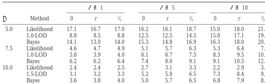
TABLE 2
Average size in centimorgans of simulated confidence intervals
D 51 D 55 D 510
j Method 0 r 1⁄
2 0 r 1⁄2 0 r 1⁄2
5.0 Likelihood 17.1 16.7 17.0 16.2 16.1 18.7 15.0 18.0 21.3 1.0-LOD 8.8 8.5 8.8 12.5 12.5 14.5 15.0 17.1 19.7 Bayes 14.1 13.0 14.0 15.3 14.8 16.9 16.3 18.0 20.9 7.5 Likelihood 4.6 4.7 4.9 5.1 5.7 6.3 5.3 6.4 7.4 1.0-LOD 3.8 3.9 4.0 6.1 6.7 7.5 8.3 9.5 10.9 Bayes 6.2 6.2 6.4 7.4 8.0 9.1 9.1 10.5 12.3 10.0 Likelihood 2.4 2.4 2.5 2.7 3.1 3.3 2.2 2.9 3.1 1.5-LOD 3.1 3.2 3.3 5.2 5.8 6.5 7.3 8.4 9.0 Bayes 3.6 3.8 4.0 5.0 5.7 6.5 6.8 7.9 8.6
Three locations for the QTL were simulated: 0 for the trait at a marker,1⁄
2for the trait midmarkers, and r
for the QTL randomly located between markers.
Both the 1.5-LOD (x56.9) support regions and the markers and the size of the region are roughly commen-surate; but whenjis large, the dense marker map pro-Bayesian credible regions provided at least 95%
cover-age under all simulated conditions. The support regions vides substantially smaller regions.
We performed similar simulations for a backcross gave the smallest confidence regions for dense maps,
while the Bayesian credible regions did the same for with essentially the same results (data not shown). The simulations were repeated with fewer tomatoes (N 5 sparse maps. The coverage probability for the support
regions obtained in the simulations is close to that pre- 100) (results not shown). The size of the region was unchanged for all methods, and all methods had the dicted by the approximation (15). The approximate
expected size provided by (B2) is close in the case of a right coverage probability when the locus was located at a marker. The coverage probability was substantially dense map, but not otherwise. The likelihood method
was conservative; and because it adapts to the observed reduced for the case of the likelihood method and the Bayes method when the trait was located midmarkers value of the likelihood ratio statistic at the putative trait
locus it resulted in the widest confidence regions for (≈80% instead of 95%). The LOD support method had a slight drop in confidence coverage (≈90%), but was small values of the noncentrality parameter but was
equivalent to the support region for the larger values more robust than the other methods.
We have also simulated support regions under the j 57.5 and 10. For all methods, the sizes of the intervals
were largest when the trait was midmarker. The Bayes conditions of Table 2 ofVisscheret al. (1996), which
involved a backcross with no dominance variance and credible sets were the widest and they fell short of the
desired 95% for large values ofjand sparse maps, espe- marker spacings of 20 cM. At this intermarker distance 1-LOD (x 5 4.6) regions had coverage probabilities cially when the trait was located at a marker.
The size of the confidence regions is relatively insensi- ranging from 93 to 96% and in all cases gave smaller regions than the 95% bootstrap regions recommended tive to the marker density when the distance between
TABLE 3
Coverage probability of simulated confidence intervals
D 51 D 55 D 510
j Method 0 r 1⁄
2 0 r 1⁄2 0 r 1⁄2
byVisscheret al. (1996), while 1.5-LOD regions had correlated than would be the case if the data were not missing, so the threshold obtained under the assump-98–99% coverage probability and about the same
ex-pected sizes as the bootstrap regions. For example, for tion of no missing data is still appropriate and, in fact, slightly conservative.
a heritability of 0.05 and a sample size of 500, which
yield a noncentrality parameterj 55.06, the coverage The assumption of normality is robust in the sense that the regression statistics we use are approximately probability of the 1-LOD region based on 1000
simula-tions was 96%, and the expected size was 29 cM com- normally distributed in large samples, so our approxi-mations for significance level and power are valid in pared with 96% and 43 cM obtained byVisscheret al.
(1996) for their bootstrap regions. large samples. However, it is possible that by using a
more appropriate model, e.g., a mixture model if the Another method to obtain confidence intervals for
QTL location has been proposed by Mangin et al. nonnormality arises from large QTL effects, one can obtain greater power, although large QTL effects will (1994). This method amounts to fixing a putative QTL
location and testing the hypothesis that there is no QTL be comparatively easy to detect with a suboptimal proce-dure.
between that location and either end of the
chromo-some. In the statistical literature on change-point analy- When using a backcross or intercross, intermarker distances up toz10 cM are almost as powerful as contin-sisWorsley(1986) has discussed a similar idea and has
pointed out that if there is another change-point (here uously distributed markers. Except at intermarker dis-tances of z20 cM or more, or when using a design QTL on the same chromosome) the method may
pro-duce an empty confidence set, since for every putative involving a large recombination rate, e.g., a recombinant inbred design or advanced intercross design, there is QTL there is evidence of another somewhere on the
chromosome. Of course, the problem of detecting a little gain in power from interval mapping, which in any event does not provide nearly as much power as more second, linked QTL given an already detected QTL is
itself interesting and important. closely spaced markers.
Although intercross designs involve a 2-d.f. statistic and hence a higher threshold than a backcross design,
DISCUSSION
and have larger residual variance, intercross designs are usually more powerful than backcross designs, unless In this article we have discussed genome scanning
methods to detect QTL in experimental genetics. Our (a) the effect of the gene is large and additive or (b) there is dominance and the dominance deviation has goal has been to produce relatively simple
approxima-tions for quantities of interest, e.g., the false-positive the same sign as the additive genetic effect. A backcross design can lose considerable power in the presence of error rate, power to detect a QTL, and coverage
proba-bility of a support region, so that one can easily address even a small departure from additivity if the incorrect parental strain is used for the backcross. A recombinant questions concerning sample size, marker density, etc.,
and can compare different designs. Our approximations inbred design can be more efficient than an intercross, except when dominance effects are large compared to for significance level and power seem adequate in this
regard, but our approximations for the expected size additive effects. Because of the high recombination rate associated with recombinant inbreds, especially those of a support region are good only for dense markers
(e.g.,D≈1 cM). based on recurrent sib mating, power to detect linkage
falls off rapidly with intermarker distance when a QTL Although in a backcross the conventional LOD 5
3 threshold produces false-positive rates,0.05 unless is located midway between markers. To avoid this loss of power when using an inbred design based on recur-intermarker distances are small, it is anticonservative in
an intercross even for intermarker distances as large as rent sib mating, intermarker distances should be no more than 5 cM and preferably should be even less. 25 cM without interval mapping.
Our approximations are based on the artificial as- Similar considerations apply to advanced intercross lines (DarvasiandSoller1995).
sumption that markers are equally spaced and there are
no missing data. If markers are not equally spaced, the We have also presented three methods of con-structing confidence regions for the location of QTL: approximations (4) and (9) can be modified by
averag-ing the function n with respect to the distribution of the likelihood method, Bayes credible sets, and support regions. The support method and the Bayesian credible the distancesDbetween markers. One can also use the
original approximations with an average intermarker sets seem roughly comparable in large samples, but the coverage probability of the support method is more distance. (This should be the average distance in the
neighborhood of detected QTL if one adds additional robust to changes in the sample size. Both methods are better than the likelihood ratio method, which often markers to promising regions.) Since (4) and (9) are
insensitive to minor changes in the assumed value of has a coverage probability substantially smaller than the nominal level, except for the case of dense markers. D, one can reasonably expect such refinements to have
in the neighborhood of the QTL. When the noncentral- of controlling the phenotypic variability due to multiple QTL, but at least initially has the disadvantage that the ity parameter isz5, which provides power ofz0.9 for
QTL detection, little is gained by having markers more success of the control depends on fortuitously placing the control markers close to true QTL. Straightforward closely spaced thanz10 cM; but when the noncentrality
parameter is 7.5, intermarker distances of 1–5 cM pro- calculations show that the control markers on other chromosomes have no effect on the asymptotic distribu-vide shorter confidence regions. A reasonable guideline
is to achieve a marker density in the neighborhood of tion of the log-likelihood ratio process along the cur-rently searched (unlinked) chromosome, although they a putative QTL about equal to the expected half length
of a support region for a QTL of that strength. do reduce the number of degrees of freedom available to estimate the error variance. By considering one chro-When dominance effects are relatively small and
markers sufficiently dense, support regions from recom- mosome at a time and adding the chromosome-wide false-positive rates, one obtains an asymptotic upper binant inbred designs are often about one-fourth as
large as from intercross designs, which in turn are sub- bound on the genome-wide false-positive rate. Because of the independent assortment of chromosomes, this stantially smaller than from backcross designs.
Ad-vanced intercross designs (DarvasiandSoller1995) upper bound should not be overly conservative. The second method discussed byDupuiset al. (1995),
are also especially powerful for fine localization of QTL.
In almost all cases, however, the size of the confidence simultaneous search, will for the reasons given there rarely be useful in the absence of epistasis. Preliminary regions is on the order of several centimorgans unless
the sample size is considerably larger than what is re- calculations suggest it can be very helpful when there is substantial epistasis.
quired to detect linkage, so there is a continuing need
to develop better designs for fine localization of QTL. We expect to return to the problem of detecting mul-tiple, possibly linked, QTL in a future article.
We have not explicitly addressed the complexities
associated with identifying multiple, possibly linked, This research was partially supported by the National Institutes of possibly interacting, QTL. For mapping qualitative traits Health grant HG-00848 and the National Science Foundation grant
DMS 9704324.
in humans, we have discussed these issues (Dupuis et al. 1995), and expect to return to them for QTL
map-ping. For example, once a linked QTL is located,
condi-LITERATURE CITED
tional search removes the effect of that QTL by
sub-tracting its (estimated) genotypic contribution from Andersson, L., C. S. Haley, H. Ellegren, S. A. Knott, M. Johansson et al., 1994 Genetic mapping of quantitative trait loci for growth
the phenotypic value to define a new regression model,
and fatness in pigs. Science 263: 1771–1774.
hence a new log-likelihood ratio statistic, to search for
Churchill, G. A.,andR. W. Doerge,1994 Empirical threshold
additional QTL. Suppose an intercross design is used values for quantitative trait mapping. Genetics 138: 963–971. Cobb, G. W.,1978 The problem of the Nile: conditional solution
and, for simplicity, we use a 1-d.f. statistic to detect a
to a change-point problem. Biometrika 62: 243–251.
QTL of purely additive effect. Assume also that we know
Conneally, P. M., J. H. Edwards, K. K. Kidd, J.-M. Lalouel, N. E. exactly the location of a QTL making contribution v2to
Mortonet al., 1985 Report of the Committee on Methods of Linkage Analysis and Reporting. Cytogenet. Cell Genet. 40: 356–
the heritability. The (asymptotic) correlation function
359.
between the new and old processes at each unlinked
Cox, D. R.,andD. V. Hinkley,1974 Theoretical Statistics. Chapman marker is (1 2 v2)1/2, and under the assumption of
and Hall, London.
Darvasi, A., andM. Soller,1995 Advanced intercross lines, an
no epistasis, the noncentrality parameter for the new
experimental population for fine genetic mapping. Genetics 141:
statistic is larger by the factor 1/(1 2 v2)1/2. Hence a
1199–1207.
large QTL effect v2 is necessary at the detected locus
Darvasi, A., A. Weinreb, V. Minke, J. I. WellerandM. Soller,
1993 Detecting marker-QTL linkage and estimating QTL gene
to get a reasonable “gain” from the conditional search,
effect and map location using a saturated genetic map. Genetics
although a large value of v2also leads to a new process
134:943–951.
only weakly correlated with the original search process, Dempster, A. P., N. M. LairdandD. B. Rubin,1977 Maximum
likelihood from incomplete data via the EM algorithm. J. R.
which increases the likelihood that conditional search
Statist. Soc. B39: 1–22.
will incur a false-positive error. Of course, there must
Dupuis, J.,1994 Statistical problems associated with mapping
com-be another QTL of sufficiently large effect for the gain in plex and quantitative traits from genomic mismatch scanning
data. Ph.D. Thesis, Stanford University, Stanford, CA.
noncentrality to be helpful. Rough calculations suggest
Dupuis, J., P. O. BrownandD. Siegmund,1995 Statistical methods
that suitable combinations of QTL effects will occur
for linkage analysis of complex traits from high resolution maps
relatively rarely. of identity by descent. Genetics 140: 843–856.
Feingold, E., P. O. BrownandD. Siegmund,1993 Gaussian models
Similar considerations are relevant to recently
sug-for genetic linkage analysis using complete high resolution maps
gested multiple regression methods, e.g.,Zeng(1994)
of identity-by-descent. Am. J. Hum. Genet. 53: 234–251.
andJansen(1994), whereby one searches, for example, a Fisher, R. A.,1934 Two new properties of mathematical likelihood.
Proc. R. Soc. A 144: 285–307.
given chromosome or chromosomal arm for a QTL while
Haley, C. S.,andS. A. Knott,1992 A simple regression method
controlling for QTL on other chromosomes through
for mapping quantitative trait loci in line crosses using flanking
arbitrarily placed markers. In comparison with condi- markers. Heredity 69: 315–324.
et al., 1991 Genetic mapping of a gene causing hypertension in decomposition the stroke-prone spontaneously hypertensive rat. Cell 67: 213–
P[max
d Zd$b]5P[Zq$b]1P[Zq, b, maxd?q Zd$b].
224.
Jansen, R. C.,1994 Controlling the type I and type II errors in
mapping quantitative trait loci. Genetics 138: 871–881. The first term on the right-hand side is given by 12
Johnstone, I. M.,andD. Siegmund,1989 On Hotelling’s formula
F(b2 jq), wherejq5E(Zq). To approximate the second
for the volume of tubes and Naiman’s inequality. Ann. Statist.
17:184–194. term, we assume that if the process exceeds the
thresh-Kempthorne, O.,1957 An Introduction to Genetic Statistics. John Wiley old for some d ?q it does so at a value of d between
and Sons, New York.
the same two flanking markers as q, or in one of the Korol, A. B., Y. I. RoninandV. M. Kirzhner,1995 Interval mapping
of quantitative trait loci employing correlated trait complexes. immediately adjoining marker intervals in the case that Genetics 140: 1137–1147. q is itself a marker. This analysis can be expected to yield
Kruglyak, L.,andE. S. Lander,1995 High-resolution mapping of
reasonable approximations in the case that intermarker
complex traits. Am. J. Hum. Genet. 56: 1212–1223.
Lander, E. S.,andD. Botstein,1986 Mapping complex genetic intervals are large, when interval mapping is supposed
traits in humans: new methods using a complete RFLP linkage to be most helpful. It may not be effective when the map. Cold Spring Harbor Symp. Quant. Biol. 51: 49–62.
intermarker distances are small, expecially if the non-Lander, E. S.,andD. Botstein,1989 Mapping Mendelian factors
underlying quantitative traits using RFLP linkage maps. Genetics centrality is also small. We approximate maxdZd by
ex-121:185–199. panding Z
din two terms of a Taylor series around d5q
Lander, E. S.,andL. Kruglyak,1995 Genetic dissection of complex
and using calculus to maximize the resulting expression.
traits: guidelines for interpreting and reporting linkage results.
Nat. Genet. 11: 241–247. SeeSiegmund andWorsley(1995) for details of this Mangin, B., B. GoffinetandA. Rebai,1994 Constructing confi- calculation. The final approximation is
dence intervals for QTL location. Genetics 138: 1301–1308.
Ott, J.,1991 Analysis of Human Genetic Linkage, Revised Edition.
P[max
d Zd$ b]≈12 F(b2 jq)
Johns Hopkins University Press, Baltimore.
Paterson, A. H., S. Damon, J. D. Hewitt, D. Zamir, H. D.
Rabino-1 Iq(jq2b)21w(b2 jq)[12 (b/jq)1/2], (A1)
witch et al., 1991 Mendelian factors underlying quantitative traits in tomato: comparison across species, generations, and
environments. Genetics 127: 181–197. where Iqequals 2 or 1 according to the trait locus being
Rebai, A., B. GoffinetandB. Mangin,1994 Approximate thresh- at a marker or in the interval between markers. This olds of interval mapping test for QTL detection. Genetics 138:
discontinuous behavior at the markers is caused by the
235–240.
Rebai, A., B. GoffinetandB. Mangin,1995 Comparing power of discontinuity in the derivative of the interval mapping
different methods for QTL detection. Biometrics 51: 87–99. statistic that occurs at the markers.
Siegmund, D.,1985 Sequential Analysis: Tests and Confidence Intervals.
The noncentrality parameter jqcan be evaluated by
Springer-Verlag, New York.
Siegmund, D.,1988 Confidence sets in change-point problems. Int. a direct computation starting from a suitable explicit
Statist. Rev. 56: 31–48. representation of the interval mapping statistic. See
Siegmund, D.,andK. Worsley,1995 Testing for a signal with
un-Rebaiet al. (1995) for such a representation in a
com-known location and scale in a stationary Gaussian random field.
Ann. Statist. 23: 608–639. plete interference model; their equation is easily modi-Stuber, C. W., S. E. Lincoln, D. W. Wolff, T. Helentjarisand fied for the Haldane model of no interference. We
pres-E. S. Lander,1992 Identification of genetic factors contributing
ent here an alternative method, which will be easier to
to heterosis in a hybrid from two elite maize inbred lines using
apply to intercross designs, where the explicit statistic
molecular markers. Genetics 132: 823–839.
Visscher, P. M., R. ThompsonandC. S. Haley,1996 Confidence is much clumsier to manipulate. We begin with the intervals in QTL mapping by bootstrapping. Genetics 143: 1013–
following asymptotically equivalent expression for the
1020.
square root of (3): Woodroofe, M.,1976 Frequentist properties of bayesian sequential
tests. Biometrika 63: 101–110.
Worsley, K. J.,1986 Confidence regions and tests for a change- R[xi(d)21⁄2](yi2y)
se{R[xi(d)2 1⁄2]2}1/2
, (A2)
point in a sequence of exponential family random variables. Biometrika 73: 91–104.
Zeng, Z.-B.,1994 Precision mapping of quantitative trait loci.
Genet-where y5 N21Ry
i. In the case where the locus d lies
ics 136: 1457–1468.
Zhang, H. P.,1991 A study of change-point problems. Ph.D. Thesis, between flanking markers, we replace the actual marker
Stanford University, Stanford, CA. data, x
i(d), by its conditional expectation given the
geno-types of the flanking markers, E[xi(d)|Gi]. Taking
ex-Communicating editor:S. Tavare´
pectations and using (2), we see from some simple ma-nipulations that the noncentrality is asymptotically equal to
APPENDIX A
[(a 1 d)/se]{RiE[E(xi(q)|Gi)2 1⁄2]2}1/2.
Power of interval mapping:We first consider a
back-cross and suppose there is a single trait locus (on any To express this explicitly in terms of recombination fractions, letu1(u2) denote the recombination fraction
particular chromosome) at q. Let Zddenote the signed
square root of twice the log-likelihood ratio (incorporat- between the QTL at q and the marker flanking on the left (right), andu the recombination fraction between ing interval mapping), which for large N behaves like