ABSTRACT
USSET, JOSEPH LOUIS. Some Regression Models and Algorithms for Functional Data. (Under the direction of Armin Schwartzman and Arnab Maity.)
This dissertation consists of three projects in the area of Functional Data Analyses (FDA) that share a common methodological framework based on extensions of generalized additive
models fit with penalized regression splines. The first project proposes methods for estimation
and prediction in a functional regression model with a scalar response and multiple functional predictors that accommodates two-way interactions in addition to their main effects. The second
project presents methods for hypothesis testing for a two-way interaction in the functional linear
model. The final project develops a method for identifying a smooth function of inflection points that lie within a time series of curves.
Chapter 2 describes the first project. It considers a functional regression model with a
scalar response and multiple functional predictors that accommodates two-way interactions in addition to their main effects. We develop an estimation procedure where the main effects are
modeled using penalized regression splines, and the interaction effect by a tensor product basis.
For comparison we present a low-dimensional estimation approach based on an extension of functional principal components regression. Extensions to generalized linear models and data
observed on sparse grids or with error are also presented. Our proposed method can be easily
implemented through existing software. Through numerical studies we investigate the effects of model mis-specification in functional linear models. We find that fitting an additive model in the
presence of interaction leads to both poor estimation performance and loss of prediction power,
while fitting an interaction model where there is in fact no interaction leads to negligible losses. We illustrate our methodology by analyzing a brain tractography data set and the AneuRisk65
data.
Chapter 3 describes the second project. It deals with the issue of hypothesis testing for a two-way interaction effect in a functional linear model with multiple functional predictors.
We develop three hypothesis testing procedures of a two-way interaction effect between two
functional predictors in a functional linear model with a scalar response. First, we propose a novel application of a recently developed Wald statistic for testing in generalized additive models
fit with penalized regression splines. Next, we consider two testing procedures that rely on low-dimensional approximations to the functional linear interaction model where the coefficients for
interaction are treated as either fixed or random effects. We provide code examples for each
procedure, and extensions to generalized linear models and data observed on sparse grids or with error are also presented. All the methods are compared through extensive simulation studies
power of the proposed tests, while the low-dimensional approach that incorporates interaction
coefficients as random effects performs second best. We illustrate our methodology on the brain tractography and AneuRisk65 data.
Chapter 4 describes the third project. It develops a statistical algorithm to identify a smooth
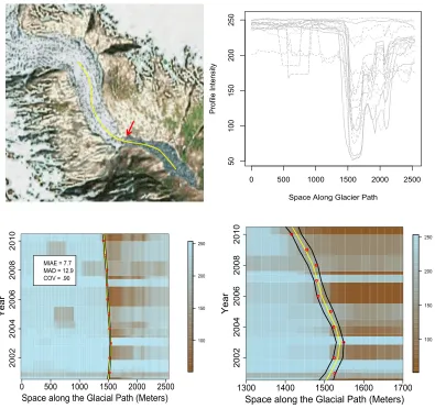
path of inflection points within a time series of curves. The scientific motivation is to build an automated way to quantify the retreat of mountain glaciers from a sequence of 1-D intensity
profiles extracted from 2-D Landsat images. The guiding assumption we make is that the glacier
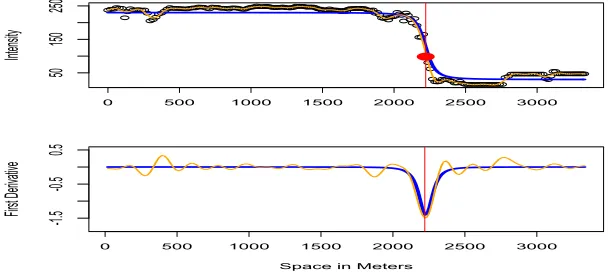
terminus lies near the point of highest inflection in the image profiles. The framework we propose has three main steps. First, the intensity profiles are smoothed with penalized regression splines,
and first derivatives of the smoothed profiles are extracted. Second, the first derivative profiles
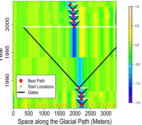
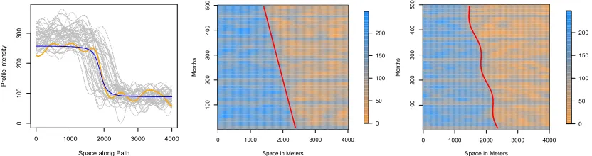
are input into a pilot path algorithm which outputs an initial estimate of the terminus location. Third, the pilot path is smoothed to identify long-term trends in the terminus movement. The
viability of our method is shown through simulation studies and applications to real data from
©Copyright 2014 by Joseph Louis Usset
Some Regression Models and Algorithms for Functional Data
by
Joseph Louis Usset
A dissertation submitted to the Graduate Faculty of North Carolina State University
in partial fulfillment of the requirements for the Degree of
Doctor of Philosophy
Statistics
Raleigh, North Carolina
2014
APPROVED BY:
Ana-Maria Staicu David Dickey
Armin Schwartzman Co-chair of Advisory Committee
Arnab Maity
DEDICATION
BIOGRAPHY
Joseph Usset was born in St. Paul, MN to Mary and Edward Usset. He graduated from Henry Sibley High School in Mendota Heights, MN in 2004 and attended St. Olaf College in Northfield,
MN where he graduated in 2008 with a B.A. in Mathematics. He moved to Raleigh, NC to join the Department of Statistics at North Carolina State University and completed a Master’s
ACKNOWLEDGEMENTS
First, I would like to particularly thank my research advisors Arnab Maity, Armin Schwartzman, and Ana-Maria Staicu. This dissertation would not have been possible without each of your time
and patience. Thank you for your encouragement, ideas and debates, and professional guidance. I also want to thank my committee member David Dickey for a willingness to share time and
perspective; and the many other amazing faculty, staff, and fellow students who have made my
time at NC State worthwhile.
This dissertation started on a hill in Minnesota, and so I want to thank my faculty advisors
from St. Olaf College. Thank you Kristina Garrett for helping me see creativity and excitement
in mathematical research, and Paul Roback for introducing me to statistics and encouraging me to apply to graduate school.
Finally, I want to thank my parents for dropping me off at Mendota Elementary many years
ago. Mom, thank you for worrying for me, and always pushing me to do my best. Dad, thank for your example, and teaching me everything from chess to baseball. I could not have asked
for better support, and I am in huge debt to both of you for the wonderful opportunities it has
TABLE OF CONTENTS
LIST OF TABLES . . . vii
LIST OF FIGURES . . . viii
Chapter 1 Introduction . . . 1
Chapter 2 Estimation of Interaction in Functional Linear Regression . . . 4
2.1 Introduction . . . 4
2.2 Methodology . . . 6
2.2.1 Fitting . . . 9
2.2.2 Standard Error Estimation . . . 10
2.2.3 Smoothing parameter selection . . . 11
2.3 Extensions . . . 12
2.3.1 Generalized Functional Interaction Models . . . 12
2.3.2 Functional Principal Components Analysis . . . 14
2.4 Functional Principal Components Regression . . . 15
2.5 Simulation . . . 16
2.5.1 Design and Assessment . . . 17
2.5.2 Simulation Results . . . 18
2.6 Applications . . . 19
2.6.1 DTI data . . . 19
2.6.2 Application to AneuRisk study . . . 21
2.7 Implementation . . . 23
2.8 Discussion . . . 24
Chapter 3 Testing for Interaction in Functional Linear Regression . . . 26
3.1 Introduction . . . 26
3.2 Methodology . . . 28
3.2.1 Wald Test . . . 28
3.2.2 Low-Dimensional Framework . . . 30
3.3 Simulations . . . 32
3.3.1 Simulation Design . . . 32
3.3.2 Implementation . . . 32
3.3.3 Simulation Results . . . 33
3.4 Data Analyses . . . 34
3.4.1 DTI . . . 34
3.4.2 Aneurisk . . . 34
3.5 Discussion . . . 34
Chapter 4 Glacier Terminus Estimation from LandSat Images . . . 36
4.1 Introduction . . . 36
4.2 Methodology . . . 39
4.2.2 The Model . . . 40
4.3 Spatial Smoothing . . . 42
4.3.1 Spline Smoothing . . . 42
4.3.2 Basis and Penalty Specification . . . 43
4.4 Pilot Path Algorithm . . . 44
4.5 Temporal Smoothing . . . 45
4.5.1 Weights . . . 45
4.5.2 Estimation . . . 47
4.6 Simulation Study . . . 48
4.6.1 Data Generation . . . 48
4.6.2 Simulation Results . . . 49
4.7 Real Data Analyses . . . 51
4.8 Discussion . . . 51
4.8.1 Alternative Directions . . . 52
References. . . 56
Appendices . . . 65
Appendix A Supplementary Material for Estimation of Interaction in Functional Linear Regression . . . 66
A.1 DTI Results . . . 66
A.2 Aneurisk Results . . . 68
A.3 Simulation Results . . . 71
Appendix B Supplementary Material for Testing for Interaction in Functional Linear Regression . . . 78
B.1 Simulation Settings . . . 78
B.2 Simulation Results . . . 79
Appendix C Supplementary Material for Glacier Terminus Estimation from Land-Sat Images . . . 84
C.1 Data Analyses . . . 84
C.1.1 Gorner . . . 85
C.1.2 Franz Josef . . . 86
LIST OF TABLES
Table 4.1 Simulation results for g1(t) . . . 50
Table 4.2 Simulation results for g2(t) . . . 50
Table A.1 Mis-classification rates for PFR interaction model in Aneurisk Data. . . 69
Table A.2 Mis-classification rates for FPCR interaction model in Aneurisk Data. . . 69
Table A.3 Simulation results when predictors are observed without error. . . 75
LIST OF FIGURES
Figure 4.1 Nigardsbreen results. . . 38
Figure 4.2 Motivation for model assumptions. . . 41
Figure 4.3 Motivation for estimation criterion. . . 42
Figure 4.4 Visual explanation of pilot path algorithm. . . 44
Figure 4.5 Simulation settings. . . 48
Figure 4.6 Jackknife confidence intervals. . . 53
Figure A.1 DTI data. . . 66
Figure A.2 PFR estimates for DTI study. . . 67
Figure A.3 FPCR estimates for DTI study. . . 67
Figure A.4 Aneurisk Data. . . 68
Figure A.5 PFR estimates for Aneurisk65 data. . . 68
Figure A.6 FPCR estimates for Aneurisk65 data. . . 69
Figure A.7 PFR estimated probabilities of group membership for Aneurisk65 data. . . . 70
Figure A.8 FPCR estimated probabilities of group membership for Aneurisk65 data. . . 70
Figure A.9 Results for situation where Gaussian data was generated from the interaction model at sample size 100. . . 71
Figure A.10 Results for situation where Gaussian data was generated from the interaction model at sample size 200. . . 72
Figure A.11 Results for situation where Gaussian data was generated from the interaction model at sample size 500. . . 73
Figure A.12 Results for situation where Gaussian data was generated from the interaction model at sample size 200, and interaction model is mis-specified. . . 74
Figure B.1 Settings for testing simulation. . . 78
Figure B.2 Quantile-Quantile plots for empirical null distribution of P-values compared to a uniform(0,1) distribution for Gaussian data simulation with n= 100. . . 79
Figure B.3 Power results for simulation from Gaussian data simulation withn= 100. . . 80
Figure B.4 Quantile-Quantile plots for empirical null distribution of P-values compared to a uniform(0,1) distribution for Gaussian data simulation with n= 250. . 80
Figure B.5 Power results for Gaussian data simulation withn= 250. . . 81
Figure B.6 Quantile-Quantile plots for empirical null distribution of P-values compared to a uniform(0,1) distribution from Binomial data simulation withn= 250. . 81
Figure B.7 Power results for the Binomial data simulation with n= 250. . . 82
Figure B.8 Quantile-Quantile plots for empirical null distribution of P-values compared to a uniform(0,1) from Binomial data simulation withn= 500. . . 82
Figure B.9 Power results for the Binomial data simulation with n= 500. . . 83
Figure C.1 Gorner results. . . 85
Figure C.2 Franz Josef results. . . 86
Chapter 1
Introduction
Functional Data Analyses (FDA) has attracted a lot of attention recently. This interest is due to modern technology that generates unprecedented amounts of high-dimensional data
across scientific disciplines. Often, these high-dimensional data arise from smooth and unknown
underlying processes; and are considered functional data. FDA are extensions of multivariate data analyses to situations where one or more of the variables of interest are functions, as
opposed to vector valued. Broadly, FDA methods leverage smoothness in the functional data
to obtain more effective dimension reduction and information extraction.
This dissertation consists of three FDA projects. Each project is motivated by data for which
standard statistical tools are not well suited. Chapters 2 and 3 consider a study that seeks to
relate the presence or absence of aneurysms on the internal carotid artery (ICA) to the ICA geometry. For each individual, the ICA geometry is described by curvature and radius profiles
evaluated along the artery centerline. Chapters 2 and 3 also include a neurological study that
relates cognitive exam scores, to brain tractography profiles which are indicators of multiple sclerosis. Chapter 4 seeks to quantify glacier recession from satellite imagery, and the data
are 1-D image profiles extracted from a 2-D Landsat images over time. The curvature, radius,
tractography, and image profiles are all functional data, and the analyses of these data sets require FDA tools.
A common theme is that proposed methods are based on extensions of tools developed for
generalized additive models (GAMs). GAMs are generalized linear models in which at least one component of the linear predictors is explained by a smooth function of the predictor variables.
An extended definition of GAMs includes situations where the unknown functions relate to the
response through a pre-specified linear functional; and this broader definition of GAMs includes regression models where the predictors are thought of as functions. Both GAMs and FDA have
The models we consider take the general form
Yi =α+
X
j
Lijfj+i, (i= 1, ..., n), (1.1)
whereY1, ..., Ynare independent responses and thefj are smooth unknown functions of interest
of one or more variables. The Lij represent bounded linear functionals which are described by
Wahba (1990). These models provide a general framework that encompasses both functional
linear regression (focus of Chapters 2 and 3) and non-parametric regression (used in Chapter
4). Each project also shares a common basis for estimation from model (1.1). The unknownfj
are expanded in terms of known bases functions
fj =
X
k
φjk(·)βjk
where theβjk are unknown coefficients of interest. The smoothness for each function is controlled
by an extra roughness penaltyβjTP˜jβj, where βj is the corresponding vector of coefficients and
˜
Pj is a pre-specified penalty matrix. The model can be written asYi =Xiθ+i, where X is a
design matrix whose ith row contains the evaluated Lijφjk, and θ is vector of coefficients that
contains α and the sub-vectors βj. For penalty matrices Pj whose only non-zero elements are
blocks ˜Pj, such thatβjTPjβj =βjTP˜jβj,θis estimated by
ˆ
θ= arg maxθ
l(θ)−
J
X
j=1
λjβjTPjβj
, (1.2)
where l(θ) is the log-likelihood and the λj are roughness penalties that control the tradeoff
between the smoothness of the function estimates and the fit to the data. The roughness
penal-ties drive model fitting, and are selected by prediction based criteria such as cross-validation,
or from a mixed model representation of the fitting procedure where the smoothing parame-ters enter as variance components. From the estimated coefficients ˆθ, the individual functional
estimates are then obtained by ˆfj =Pkφjk(·) ˆβjk.
A recurring challenge is producing reliable inferential procedures for the function estimates, both in terms of point-wise intervals and hypothesis tests. This difficulty is the cost of flexibility
provided by GAM estimation with penalized splines. While GAMs provide a rich framework for estimation, the roughness penalties induce bias into the fitting procedure. This bias disrupts
standard inferential tools for linear models and generalized linear models (GLMs), and if left
un-accounted for, leads to under-estimation of the uncertainty in parameter estimates. Therefore, in each project we follow a Bayesian approach to obtain interval estimates and develop hypothesis
Chapter 2 focuses on estimation in a model with a scalar response and two functional
predictors that accommodates two-way interactions in addition to their main effects. The main effects of the functional predictors on the mean response is quantified by the inner product
of the individual predictors with unknown main effect functions β1 and β2; while the effect
of interaction is modeled as the inner product of the point-wise product of the functional predictors with an unknown bi-variate function γ. Extensions to generalized linear models and
data observed on sparse grids or with error are also presented. For comparison purposes, we
consider a low-dimensional approach based on an extension to Functional Principal Components Regression (FPCR). We evaluate our methodology through extensive simulation study, and also
illustrate the procedure on a brain tractography data set and the AneuRisk65 study data.
Chapter 3 considers the issue of hypothesis testing for a two-way interaction effect in between two functional predictors in a functional linear model. We develop three procedures for testing
hypotheses a two-way interaction effect between two functional predictors in a functional linear
model with a scalar response. The first approach we propose is an natural extension of the penalized spline based estimation procedure described above, where a test statistic is developed
that is based on a Bayesian approach to uncertainty estimation. For comparison we also develop
testing procedures based on a low-dimensional representation of the functional linear model, where the coefficients for interaction enter as either fixed or random effects. The test procedures
are extended to the generalized linear models settings, and to scenarios where the functional covariates are measured with error or on a sparse grid.
Chapter 4 develops a method to detect a smooth path of change points from a time series
of continuous curves. This goal of this project is to develop an automated way to track glacial recession from satellite imagery. The proposed method simplifies the problem from 2-D to
1-D by extracting spatial image intensity profiles along the inlets in the glacier, and tracking
the glacier terminus over time. For each intensity profile we apply non-parametric regression and inflection points in the regressor functions are seen as potential candidates for the terminus
location. A pilot algorithm is used to identify the best candidate for the glacier terminus location
over time. Finally, nonparametric regression is applied to the temporal sequence of estimated terminus locations in order to quantify the long-term trend in the glacier’s retreat. Our method
is shown to be effective through both simulation study, and real data analyses of the Gorner,
Chapter 2
Estimation of Interaction in
Functional Linear Regression
2.1
Introduction
Functional linear regression models with scalar response and functional covariates have received
a significant amount of attention in literature since its introduction by Ramsay and Dalzell (1991). A typical functional linear model with a single functional predictor quantifies the effect
of the predictor as an inner product between the functional predictor and an unknown
coeffi-cient function. Estimation of the coefficoeffi-cient is done using basis expansions using pre-specified basis functions, e.g., spline or Fourier bases, or empirical eigenbasis functions. Estimation and
inference on this model is well studied, see for example, Frank and Friedman (1993), Cardot
et al. (2003b) and Hall and Horowitz (2007). There have been several extensions to the func-tional linear models, including nonparametric dependence for the predictors (Ferraty and Vieu,
2002); parametric models with quadratic dependence (Yao and M¨uller, 2010), additive
regres-sion models accounting for linear main effects of multiple predictors (James, 2002; Goldsmith et al., 2011; Gertheiss et al., 2013) as well as nonlinear additive models (Ferraty and Vieu, 2009;
Chen et al., 2011; Fan and James, 2012). However, all the above mentioned literature consider only main effects, whether linear or nonlinear, of the functional predictors, and do not account
for a possible interaction effect between two different functional covariates. The main focus of
this chapter is a functional linear regression model that accounts for a two-way interactions in addition to the main effects of the functional variables.
The model we consider is defined as follows. Suppose for i= 1, . . . , n, we observe a scalar
X1i(·) andX2i(·) observed without noise, on dense grids. We propose the model
E[Yi|X1i, X2i] =α+
R
X1i(s)β1(s)ds+
R
X2i(t)β2(t)dt+
R R
X1i(s)X2i(t)γ(s, t)dsdt, (2.1)
where α is the overall mean, β1(·) and β2(·) are real-valued functions defined on τ1 and τ2 respectively, and γ(·,·) is a real valued bi-variate function defined on τ1×τ2. The unknown functions β1 andβ2 capture the main effects of the functional covariates, while γ captures the interaction effect. To gain some insight, consider the particular case β1(·) ≡β01, β2(·) ≡ β02, γ(·,·) ≡γ0, for scalars β01, β02,and γ0. This case reduces to the common two-way interaction model, with covariates ¯Xji =
R
Xji(s)ds, which act as a sufficient summaries, Xji, j = 1,2.
Thus the proposed model is an extension of the common two-way interaction model from scalar
covariates to functional covariates. The denseness of the sampling design and the noise free assumption are made for simplicity and will be relaxed in later sections.
Recently, Yang et al. (2013) introduced a class of functional polynomial regression models
of which model (2.1) is a special case. They showed that accounting for a functional interac-tion effect between of depth spectrograms and temperature time series improved predicinterac-tion of
sturgeon spawning rates in the Lower Missouri river. The proposed methodology relies on an
orthonormal basis decomposition of the functional covariates and parameter functions, com-bined with stochastic search variable selection in a fully Bayesian framework. This approach
requires full prior specification of several parameters, along with implementation of an MCMC
algorithm for model fitting.
Due to the developments of Yang et al. (2013), the contribution of this chapter is a novel
approach to estimation, inference and prediction in a functional linear model that includes a two-way interaction. We consider a frequentist view and model the parameter functions using pre-determined spline bases and achieve dimension reduction with shrinkage as opposed to
se-lection. The proposed method is close in spirit to Goldsmith et al. (2011), who consider only
additive effects of the functional covariates. The inclusion of an interaction term between the functional predictors involves additional computational and modeling challenges, which we
dis-cuss throughout the chapter. The main advantage of our approach is that it can be implemented
with readily available software, that accomodates 1) responses from any exponential family, 2) functional covariates observed with error, or on a sparse or dense grid, and 3) produces
p-values for individual model components, which include the interaction term. We also include a
numerical comparison between the additive and interaction functional models involving scalar response. Our findings can be summarized as follows. When the true model contains an
interac-tion between the funcinterac-tional covariates, as specified in (2.1), then fitting a simpler additive model (Goldsmith et al., 2011) leads to biased estimates and low prediction performance compared
then with sufficient sample size, fitting the more complex functional interaction model does not
harm the estimation, inference or prediction performance.
The remainder of this chapter is as follows. In Chapter 2.2, we motivate and develop the
es-timation framework for model (2.1). Chapter 2.3 extends the methodology to handle outcomes
from any exponential family and situations where predictors are measured sparsely or with er-ror. In Chapter 2.4 we briefly present an alternative low-dimensional framework for estimation,
that is used for comparison in data analyses. Chapter 2.5 consists of a simulation study that
focuses on the effects of model mis-specification. Chapter 2.6, we apply the interaction model to a publicly available tractography data set, and the AneuRisk65 data. Details about
imple-mentation are provided in Chapter 2.7. We end with a discussion that emphasizes directions
for future research in Chapter 2.8.
2.2
Methodology
We first discuss the case when the response variableY is continuous and the covariates,X1(·) and X2(·), are observed on a dense design and without noise. In chapter 2.3, we generalize our procedure to accommodate noisy and/or sparely observed predictors as well as generalized
response variables. The central idea behind our approach is to model the parameter functions using pre-specified spline bases and then use a quadratically penalized estimation procedure to
control smoothness of the estimates.
We consider basis function decompositions of the parameter functions using known spline bases. Specifically, let{ψ1k(s)}Kk=1 and {ψ2l(t)}Ll=1 be spline bases in L2(τ1) andL2(τ2) respec-tively, and furthermore let {φkl(s, t) = ψ1k(s)ψ2l(t)}1≤k≤K,1≤l≤L be the corresponding tensor
product basis in L2(τ1×τ2). We assume the representations:
β1(s) =
K
X
k=1
ψ1k(s)η1k; β2(t) =
L
X
l=1
ψ2l(t)η2l, γ(s, t) = K
X
k=1
L
X
l=1
φkl(s, t)νk,l;
where η1k’s,η2l’s, and νk,l’s are the corresponding coefficients, which are unknown. Thus
esti-mation of the parameter functions is reduced to estiesti-mation of the unknown coefficients. Using
the basis function expansions we write
R
X1i(s)β1(s)ds=PKk=1η1k
R
X1i(s)ψ1k(s)ds≈PKk=1η1ka1k,i
where a1k,i ≈
R
X1i(s)ψ1k(s)ds is calculated by numerical integration techniques; see for
ex-ample Goldsmith et al. (2011) who employ a similar technique. Similarly, we have RX2i(t)
β2(t)dt ≈ PL
l=1η2la2l,i and
R
X1i(s)X2i(t)γ(s, t)dsdt ≈ PKk=1PLl=1νk, la3k,l,i, where a2l,i ≈
R
X2i(t)ψ2k(t)dt and a3k,l,i ≈ {
R R
nu-merically. The assumption that the functional covariates are observed on dense grids of points
ensures that the integrals are approximated accurately.
To control the smoothness of the parameter functions, we take the established approach
of considering rich spline bases to model the parameter functions and drive fitting with added
“roughness” penalties to the least squares fitting criterion (Eilers and Marx, 1996; Ruppert, 2002; Cardot et al., 2003b; Eilers and Marx, 2005; Reiss and Ogden, 2010). The key assumption
in this approach is that the bases are flexible enough to capture the true parameter functions,
and that the penalties are large enough to avoid over-fitting. Letη1= (η11, . . . , η1L)T; similarly
defineη2and ν. Then the parametersα, η1, η2 andν are estimated by minimizing the penalized
criterion:
Pn
i=1(Yi−α−a1T,iη1−aT2,iη2−aT3,iν)2+P1(λ1, η1) +P2(λ2, η2) +P3(λ3, λ4, ν), (2.2)
whereYiis the observed response for individuali,a1,iis theK-dimensional vector ofa1k,i,a2,iis
theL-dimensional vector ofa2l,i, anda3,iis theKL-dimensional vector ofak,l,i;P1(λ1, η1), P2(λ2, η2),
andP3(λ3, λ4, ν) are penalty terms, andλ1, λ2, λ3, andλ4are corresponding smoothing
parame-ters. As is common in functional data we control smoothness by penalizing the derivatives of the
parameter functions. Generally speaking, we use penalties based on integratedpthorder deriva-tives, that is, Pj(λj, ηj) =λj
R {∂pβ
j(s)/∂sp}2ds,j = 1,2 are the penalty terms corresponding
to the main effects of the functional covariates, and
P3(λ3, λ4, ν) =λ3
Z Z {∂
p
∂spγ(s, t)}
2dsdt+λ 4
Z {∂
p
∂tpγ(s, t)}
2dsdt (2.3)
is the tensor product penalty corresponding to the interaction term. Defineψ(p)(·) =dpψ(·)/dtp for some generic functionψ(·). Then it is easily seen thatP1(λ1, η1) =λ1η1TP1pη1andP2(λ2, η2) = λ2ηT2P2pη2; where P1p =
R
ψ1(p)(s){ψ1(p)(s)}Tdsand P2 p =
R
ψ2(p)(t){ψ2(p)(t)}Tdt; withψ(p)
1 (s) = (ψ11(p)(s), ..., ψ(1pK)(s))T and ψ(p)
2 (t) = (ψ (p)
21(t), ..., ψ (p)
2L(t))T. For the tensor product penalty for
interaction, it can be shown (see for example Wood (2006a) Chapter 4.1.8) thatP3(λ3, λ4, ν) =
νT{λ3P1p⊗IK+λ4IL⊗P2p}ν .
Many authors have chosen to penalize integrated squared second derivatives, i.e. p= 2, for
fitting (2.2); see for example Ramsay (2005). However, in this chapter we favor penalties on the
integrated squared first derivatives, i.e. p = 1; see also Gertheiss et al. (2013) who considered this idea. Our main argument for this choice is that the first derivative penalty directly penalizes
deviations from a simpler model where the functional predictors are summarized in terms of their
average values. Infinite penalties enforce constant parameters, say β01, β02 and γ0, and revert the model back toYi=α+ ¯X1iβ01+ ¯X2iβ02+ ¯X1iX¯2iγ0+i - a standard two-way interaction
penalizing the first derivatives shows preference for the simpler interaction model. Moreover, we
have found in simulation, that with an interaction term in the model, penalties on the second derivatives tend to produce under-smoothed estimates.
Tensor Product or Thin Plate Regression Spline for Interaction?
In this chapter, we propose a tensor product basis and penalty combination to model the
interaction contour. This approach has precedence in the bi-variate functional linear regression (Marx and Eilers, 2005). Tensor product bases are attractive because they are computationally
efficient, can be constructed from any univariate bases, and easily extend to higher dimensions
(de Boor, 1978; Wood, 2006a). However, their key characteristic is separate smoothing ofγ(s, t) in each direction s and t. A drawback is that separate smoothing requires an extra penalty
parameter, which adds complexity to the model.
A computationally viable alternative to tensor products is to incorporate interaction with a thin plate regression spline. This approach has also been applied successfully in the bi-variate
functional linear regression (Reiss and Ogden, 2010). Thin plate regression splines (Wood,
2003) are reduced rank approximations to thin plate spline bases (Duchon, 1977); that are more computationally efficient. Thin plate regression splines have several appealing qualities
that make them attractive for incorporating interaction. First, due to their derivation from
thin-plates splines they avoid the problem of knot placement. Second, they require the use of only one smoothing parameter. This stems from the main assumption of thin-plate regression
splines - γ(s, t) is equally smooth in each direction s and t. For penalizing the second order
roughness functional the penalty takes the form
P(γ, λ) =λ
Z Z {[∂
2
∂s2γ(s, t)]
2+ 2[ ∂2
∂s∂tγ(s, t)]
2+ [∂2
∂t2γ(s, t)] 2}dsdt
One limitation of the thin plate regression splines is that for technical reasons the derivative penalty should be greater than one when penalizing a bi-variate surface. Therefore penalization
of integrated first derivatives, that penalize deviations from simpler models where the functional
predictors are summarized as continuous covariates, are not allowed.
Whether the interaction contour requires separate smoothing in each direction sand tis a
question for the data modeler. As a rule of thumb, if the functional predictorsX1(s) andX2(t)
have different levels of wiggliness, or are observed on different scales, it is advisable to use the tensor product approach. However, the primary reason we have focused on the tensor product
approach in this chapter is a practical one. The tensor product approach was the first that we
splines can be used to fit the model, we do not know how to extract estimated parameters.
In the data applications we have attempted both approaches has given highly similar results. Moreover, model selection criteria such as the generalized cross validation (GCV), Aikaike’s
criterion, etc. can be used to aid decisions. For the rest of this chapter assume we use the tensor
product basis and penalty.
Limitations of Model Fitting
It is clear we can estimate β1(·), β2(·) and γ(·,·) as far as they lie in the span of the pre-specified bases, but another important limitation exists for the model fitting. The unknown
parameter functions can be identified uniquely only up to the projections onto the respective spaces that generate the X1i, X2i, and X1iX2i. For example, the true β1(·) may not be re-covered completely; instead only it’s projection on the space defined by the curves X1i(·) will
be estimated. To see this, imagine a case where all X1i(·) lie in a finite dimensional space, say
X1i(s) =Pq`=1ξ1i`Φ`(s) for some orthogonal basis inL2(τ1),{Φ`(·)}`. Ifβ1(s) =β10(s)+ζΨq0(s)
such that<Ψq0,Φ` >L2= 0 for all 1≤`≤q, then we have RX1i(s)β1(s)ds=RX1i(s)β10(s)ds.
The situation is similar for the other two smooth effects, β2 and γ. While this is a conceptual limitation it relates to a practical issue in model fitting. Over regions where X1i(·),X2i(·), and
X1i(·)X2i(·) tend to be flat, it is difficult to pick up anything but constant signals. Whereas
regions over which the covariates are highly variable have the potential to identify richer signals.
2.2.1 Fitting
The criterion in (2.2) has an available analytical solution. Stack the column vectors defined
from (2.2) into individual design matrices A1 = [a11|...|a1n]T, A2 = [a21|...|a2n]T, and A3 =
[a31|...|a3n]T. Then combine these into an overall model design matrix A = [1|A1|A2|A3], and defineSλ to be a block diagonal matrix with blocks [0,λ1P1,λ2P2,{λ3P1⊗IK+λ4IL⊗P2}]. By the standard ridge regression formula we obtain parameter estimates ˆθ = ( ˆα,η1,ˆ η2,ˆ νˆ) = (ATA+Sλ)−1ATY, and by extracting ˆη1,ηˆ2, and ˆν we obtain
ˆ β1(s) =
K
X
k=1
ψ1k(s)ˆη1k; βˆ2(t) =
L
X
l=1
ψ2l(t)ˆη2l; ˆγ(s, t) = K
X
k=1
L
X
l=1
φkl(s, t)ˆνk,l. (2.4)
Predicted values for the response are obtained by
ˆ
Y =A(ATA+Sλ)−1ATY =HλY. (2.5)
Here Hλ represents the hat or influence matrix, which is important in Chapter 3.1 when
choice of the smoothness parameters. We discuss this issue in Section 2.2.3.
2.2.2 Standard Error Estimation
Estimation of confidence bands using penalized splines is a delicate issue (see Ruppert et al. (2003), Chapter 6). A straightforward approach is to construct approximate point-wise errors
bands on the frequentist covariance matrix Cov(ˆθ) = (ATA+Sλ)−1ATA(ATA+Sλ)−1σ2.This
is the approach presented by Ramsay (2005) (Chapter 15) in their treatment of the simple
functional linear model, and has also been used in the context of non-parametric regression
(Hastie and Tibshirani, 1990; Eilers and Marx, 1996; Goldsmith et al., 2011). However, we find in the simulation study of section 2.5 that confidence bands based on this covariance
often provide point-wise under-coverage. This problem has been noticed previously for
non-parametric additive models (Wood, 2006a), and for functional linear models (Goldsmith et al., 2011; McLean et al., 2012). Such under-coverage can be attributed to several important factors.
First, the penalized fitting procedure provides biased estimates of θ whenever θ 6= 0. Second, the fitting is conditional on the smoothing parameters whose uncertainty is not taken into account. Third, the level of bias induced by the penalty parameters can vary over the domain
of the functional parameters. One possible alternative to account for bias is to use the Bayesian
standard errors first proposed for smoothing splines by Wahba (1983) and cubic splines in Silverman et al. (1985). By specifying an improper prior, fθ(θ) ∝ e−θ
TS
λθ, it can be shown that θ|Y, λ ∼N(ˆθ,(ATA+Sλ)−1σ2) (see Wood (2006a), Section 4.8). The matrix CovB(ˆθ) =
(ATA+Sλ)−1σ2 is known as the Bayesian covariance matrix. This matrix can be decomposed:
CovB(ˆθ) =
Σαˆ Σα,ˆηˆ1 Σα,ˆηˆ2 Σα,ˆˆν
Σα,ˆηˆ1 Σηˆ1 Σηˆ1,ηˆ2 Σηˆ1,ˆν
Σα,ˆηˆ2 Σηˆ1,ηˆ2 Σηˆ2 Σηˆ2,ˆν
Σα,ˆνˆ Σηˆ1,νˆ Σηˆ2,νˆ Σˆν
= (ATA+Sλ)−1σ2, (2.6)
to obtain standard errors for the parameter estimates. The Bayesian formulation to the co-variance for the estimates of ˆθ is important because we use it to obtain confidence intervals.
For example, if we consider φ(s, t) = [φ1(s, t), ..., φKL(s, t)] we can obtain the covariance for
interaction Σγˆ(s,t)=φ(s, t)TΣνˆφ(s, t). Intervals are found from ˆγ(s, t) ∼N(E[ˆγ(s, t)],Σγˆ(s, t)) by standard linear models tools.
Wahba (1990) (Chapter 5) presents Bayesian confidence intervals in a general framework that contains the functional linear models; but theoretical and numerical studies of the finite
sample properties of these intervals have focused on non-parametric regression. Nychka (1988)
gaus-sian non-parametric setting. Marra and Wood (2012) studied coverage properties in the multiple
component case, where intervals are allowed to have variable width, and discussed the effects of identifiability issues. Gu and Wahba (1993) is the only work that studies coverage properties for
an interaction term, but again this focuses on the non-parametric regression setting (functional
ANOVA). Broadly, these studies conclude the main issue for proper interval coverage, in the across-the-function sense, is that the bias must only represent a modest fraction of the
over-all mean squared error. The finite sample properties of Bayesian intervals in functional linear
models is open research. We evaluate and compare the performance of both the Frequentist and Bayesian intervals in Section 2.5.
2.2.3 Smoothing parameter selection
Smoothing parameter selection is pivotal to model fitting. The smoothing parameters deter-mine the trade-off between the model’s fidelity to the data and the smoothness of the estimated
parameter functions. There are three main classes of approaches to select the smoothing
pa-rameters available within the mgcv software implementation described in Section 2.7. In this section we describe each approach and discuss which we prefer.
The first general approach is based off minimizing the expected mean square error of the
model. The un-biased risk estimation (UBRE) and equivalently Mallows’Cp criterion fall into
this class of approaches. As discussed in Wood (2006a) (Chapter 4.5.1) the goal is to minimize
E(M) =E(kµ−HλYk2)/n=E(kY −HλYk2)/n−σ2+ 2tr(Hλ)σ2/n,
whereM represents the expected mean squared error andHλ represents the hat matrix shown
in (2.5). The challenge is that the above expression contains the residual variance, σ2, which is
unknown. This criterion performs poorly when σ2 is unknown, which is often the case.
A second class of approaches attempt to minimize the mean square prediction error P =
M+σ2 (Wood (2006a) Chapters 4.5.2). To estimateP the standard is to use cross validation.
The most straightforward form of this is the leave-one-out (LOO) cross-validation procedure
Vo(λ) =
1 n
n
X
i=1
(Yi−HλY(−i))2,
where Y(−i) represents the response vector with the ith subject removed. The LOO cross-validation criteria can be rewritten
Vo(λ) =
1 n
n
X
i=1
(Yi−HλYi)2
(1−Hλ,ii)2
In the functional regression literature this approach was first used by Marx and Eilers (1999)
for simpler model with only one smoothing parameter. The main problem is that minimizing Vo for model (2.2) requires a computationally intensive grid search over multiple smoothing
parameters. A second weakness of ordinary cross-validation is a lack of invariance to orthogonal
rotations of the fitting procedure (Golub et al. (1979), Craven and Wahba (1978), Wood (2006a) Chapter 4.3). These issues motivate generalized cross validation (GCV):
Vg(λ) =
nkY −HλYk2
[n−tr(Hλ)]2
. (2.7)
For functional linear regression GCV was proposed by Cardot et al. (2003b). GCV can be
seen as ordinary cross-validation on an nice orthogonal rotation of the fitting problem that
gives equal leverage to each observed point in the data (Wahba, 1990; Wood, 2006a). The primary advantage of GCV is that (2.7) can be optimized numerically over multiple smoothing
parameters. This optimization is done in mgcv using a combination Newton’s method backed by steepest descent (for details see Wood (2004), Wood (2006a) Chapters 4.6-4.7).
The final approach to smoothing parameter selection is based on transforming the
penal-ized criterion in (2.2) into an analogous mixed model, where the smoothing parameters enter
as variance components. The variance parameters are then estimated by restricted maximum likelihood (REML) (Ruppert et al., 2003). While asymptotically prediction error criteria
pro-vide superior predictor error performance than likelihood based methods (Wahba, 1985), it is
generally known that GCV can often lead to severe under smoothing in finite samples (Wahba, 1985; Gu, 2002; Ruppert et al., 2003). Reiss and Ogden (2007) found REML yielded superior
results to GCV in simulation studies in their study of penalized functional principal components
regression, and this motivated Reiss and Ogden (2009) to analytically compare the GCV and REML criteria for finite samples. The comparison showed that relative to GCV; REML
esti-mates were less prone to multiple minima, had reduced smoothing parameter variability, and
offered overall greater resistance to over-fit. We use REML to select smoothness parameters for the Gaussian data in our simulation in Section 2.5.
2.3
Extensions
2.3.1 Generalized Functional Interaction Models
Consider the case when the outcomeYi is generated from an exponential family EF(ϑi, %) with
dispersion parameter % such that E{Y|X1i(·), X2i(·)} = g−1(ϑi), where the linear predictor
ϑi = α+
R
X1i(s)β1(s)ds+
R
X2i(t)β2(t)dt+
R R
X1i(s)X2i(t)γ(s, t)dsdt and g(·) is a known
used for the unknown parameter functionsβ1, β2, andγ. The linear predictor can be simplified
to ϑi = α+PKk=1η1ka1k,i+PLl=1η2la2l,i+PKk=1PLl=1νk,la3k,l,i, where K and L are chosen
sufficiently large to capture the variability in the parameter functions. We estimate the model
components by minimizing (2.2) with the understanding that the sum of squares criteria is
replaced by the model deviance. For given smoothing parameters there is a unique solution which can be obtained by a penalized version of iteratively re-weighted least squares (Wood,
2006a).
Inference for the non-Gaussian case can proceed from large sample results, that again can take either a frequentist or Bayesian viewpoint. Asymptotic normality of these estimators based
on the frequentist view can be obtained (Cox and Hinkley, 1979). However, this approach
suffers from the bias in the estimation procedure discussed in Section 2.2.2. The ‘Bayesian’ standard errors of Wahba (1983) and Silverman et al. (1985) have been extended to
non-Gaussian settings in non-parametric regression by (Gu, 1992; Gu and Wahba, 1993; Ruppert
et al., 2003; Wood, 2006c; Gu, 2013). Wood (2006c) shows that in the asymptotic limit θ|Y ∼
N(ˆθ,(ATW A+Sλ)−1σ2), where ˆθ is the minimizer of an analog to (2.2) and the matrix W
has diagonal entries Wii =g0(ϑi)2V(ϑi))−1: where V is the function such that V(ϑi)σ2 is the
variance ofY, whereσ2is the scale parameter. In the context of generalized additive models fit by penalized regression splines, the ‘across-the-function’ coverage properties of these Bayesian
intervals was studied by Marra and Wood (2012). These intervals have not been studied in the context of any functional linear regression. As in the gaussian case, these intervals are
conditional on the estimated smoothing parameters.
Smoothing Parameter Selection for GLMs
Recall in Section 2.2.3 we preferred REML for smoothing parameter selection in Gaussian
models. In generalized linear models (GLMs) the analog to this is PQL, where the REML (or ML) criteria is applied iteratively to working linear approximations of the likelihood. However,
a problem with this approach is that iterations fail to converge in many applications (Wood, 2011). This non-convergence issue is especially bad for binary data (Breslow and Clayton, 1993;
Wood, 2004).
A viable alternative is to base smoothness parameter selection on GCV. For GLMs, the analog to (2.7) is based on
Vg(λ) =
nD(ˆθ) [n−τ]2,
least squares at convergence. Wood (2008) provides technical optimization details and shows
through simulation and practical examples that it performs superior to PQL.
Recently, Wood (2011) proposed an efficient and stable methodology to select the smoothing
parameters for GLMs based on REML. The main idea is to avoid convergence issues of PQL
by first applying a Laplace approximation to the model likelihood, and then select smoothing parameters with REML; as motivated by Reiss and Ogden (2009). This approach was shown
to have huge advantages over PQL; and modest advantages over GCV of Wood (2008); in
simulation studies. We apply this method to determine smoothness for the logistic regressions performed in the simulation and data analyses in Sections 2.5 and 2.6.
2.3.2 Functional Principal Components Analysis
In real world situations, the true functional predictors, X1i(s) and X2i(t), are unknown and
observed discretely. Often these discretely observed curves lack smoothness due to either
mea-surement error; or because they have been evaluated at sparse and/or irregular design points
such that the set of all evaluated points is on a dense grid. Following the established frame-work of penalized function regression (Goldsmith et al., 2011); in this situation estimation is
a two-stage procedure in which the first stage is to predict the true functional predictors with
Functional Principal Component Analysis (FPCA). The basic aim of FPCA is to decompose the space of the functional predictors into basis functions which explain principal directions of
their variation. These derived basis functions can be used to predict the true unobserved
pre-dictors. There are multiple approaches to FPCA in the literature (Staniswalis and Lee, 1998; Yao et al., 2003; Di et al., 2009; Goldsmith et al., 2013)). For completeness we describe the
general framework for FPCA, and the specific approach we prefer.
For j= 1,2, given predictorsXji(s) define the covariance operator ΣjX(s, s0) = Cov[Xji(s),
Xji(s0)]. By Mercer’s theorem this covariance operator can be expressed by the spectral
de-composition ΣXj (s, s0) =P∞
k=1λjkϕjk(s)ϕjk(s0), where {λjk, j ≥1} are decreasing eigenvalues
withP∞
j=1λjk <∞and ϕjk(s) are the eigen-functions that represent the principal component
bases of interest. By Karhunen-Loeve (KL) we can expandXji(·) =Pk∞=1ξikϕjik(·), where the
corresponding functional principal component scores ξjik =
R
Xji(s)ϕjk(s)dt have mean zero
and are uncorrelated with variance λjk.
FPCA approaches are diverse due to various scenarios over which the functions are observed;
such as with measurement error or on sparse grids at the subject level. For example, measure-ment error makes the estimate of ΣX
j (s, s0) too rough, and so a common first step is to smooth
the estimated covariance matrix. Moreover, in practice, the KL expansion is truncated and
pre-dictors are approximated by Xji(·) ≈ PKk=1j ξikϕjik(·); a common criterion for the truncation
ξjik =
R
Xji(s)ϕjk(s)dt are approximated over the evaluated grid points. For data observed on
dense grids Riemann sum approximations work well, but for sparse data at the subject level a better alternative is to predict the scores as random effects in a mixed model framework
(Crainiceanu et al., 2008). We implement FPCA with the fpca.sc function in refund; this approach smooths the covariance matrices with bi-variate penalized splines, chooses by default the truncation lag according to 99% variance explained, and approximates principal component
scores as best linear unbiased predictors in a mixed model framework (Di et al., 2009; Goldsmith
et al., 2013). For a fuller review of FPCA see both Ramsay (2005) and Di et al. (2009).
2.4
Functional Principal Components Regression
Functional principal components regression (FPCR) is an alternative approach to our method that can be extended to incorporate interaction into the functional linear model. Traditionally
FPCR uses a low-dimensional principal component bases to model both the predictors and
main effect coefficient functions. To incorporate interaction, we use the tensor product of the principal component bases derived fromX1(s) andX2(t). We describe how to extend FPCR to
incorporate interaction more formally here.
For i = 1, ..., n we assume that X1i(s) = PKk=1ξikϕ1k(s) and X2i(t) = PLl=1ξikϕ2l(s).
Here for k = 1, ..., K and l = 1, ..., L the functions ϕ1k(s) and ϕ1l(t) represent the principal
component bases andξikandξiktheir corresponding scores that are estimated by FPCA. Instead
of spline modeling, the principal component basesϕ1k(s) andϕ2l(t) are used to directly model
the parameter functions
β1(s) =
K
X
k=1
ϕ1k(s)η1; β2(t) =
L
X
l=1
ϕ2l(t)η2; γ(s, t) =
K X k=1 L X l=1
ϕ1k(s)ϕ2l(t)γkl;
where theηjk’s andγjk’s are unknown coefficients of interest. Since the the principal component
bases are orthonormal, one can show the original regression model from (2.1) can be re-expressed
E[Yi|X1i, X2i] =α+ K
X
k=1
ξikη1k+ L
X
l=1
ξilη2l+ L X l=1 K X k=1
ξilξikγkl. (2.8)
From this simplified linear model representation, the standard tools for estimation, inference,
and prediction apply. In these applications it is recognized that fitting is conditional on the
estimated principal component bases and scores. FPCR is an un-penalized and low dimensional approach to functional linear regression. Instead of extra roughness penalties, the truncation
lags K and L tune the trade-off between bias and variance in the model. The truncation lags
2000). FPCR can also be easily extended to the generalized linear model setting, and to handle
extra covariates in the model. Finally, using the covariance matrix for estimated coefficients, and the fixed principal component bases ϕ1k(s) and ϕ2l(t), point-wise confidence intervals can
be estimated for the parameter functions using the methods described in 2.2.2.
To the best of our knowledge, FPCR has not been extended to incorporate interaction in the functional linear model, where estimation follows a frequentist framework. However, the
recent work of Yang et al. (2013) proposed methodology that combines FPCR with stochastic
search variable selection in a fully Bayesian framework. Also, Sangalli et al. (2009) propose the use of a classification procedure that incorporates FPC scores and their point-wise products.
It is also worthwhile to note that Reiss and Ogden (2007, 2010) proposed a penalized
version of FPCR for functional linear regression. This hybrid methodology starts with the fitting framework in 2.2, but then performs on PCA on the design matrix from 2.2. The principal
components rotation is then used to rotate the pre-specified quadratic penalties. A drawback
of this approach is that both the roughness penalties and the number of FPCs are tuning parameters in the model, that need to be chosen in combination. When the model contains
multiple functional predictors, and an interaction term is included, the computational burden
of tuning parameter selection makes this approach unappealing.
2.5
Simulation
In this section we perform a numerical study of our method. The primary objective of this simulation is to evaluate methodology described in 2.2, in terms of both parameter estimation
and predictive performance. The functional parameter estimates are evaluated in terms of the
1) bias, 2) consistency, and 3) confidence interval coverage. Prediction is assessed in terms of estimates of the residual variance and mis-classification rates. A secondary objective of this
study is to demonstrate the effects of model mis-specification. The results show that fitting a
purely additive model when interaction is present may lead to biased estimates but fitting our approach when the true model is in fact additive does not result in significant loss of accuracy
in estimation.
A couple of notes before we go into details about this simulation. A motivation for this
simulation study is the difficulty obtaining of theoretical results for the model in 2.1. Also, this
simulation has limitations. To be cautious inferences should only be made broadly to the data generative settings described next. Regardless, this numerical study serves as a rough tool for
2.5.1 Design and Assessment
The functional covariates Xji(s) =φTj(s)ξji, j = 1,2, are generated so thatξ1i ∼M V N(0,Σ)
andξ2i ∼M V N(0,Σ) with Σ = diag(8,4,4,2,2,1,1), andφ1(s) = [1,sin(πs),cos(πs),sin(3πs),
cos(3πs),sin(4πs),cos(4πs)] andφ2(t) = [1,sin(πt),cos(πt),sin(2πt),cos (2πt),sin(4πt),cos(4πt)]. We generate the observed functional covariates both with and without independent
measure-ment error, according to the model W1i(s) =X1i(s) +δ1i(s) and W2i(t) =X2i(t) +δ2i(t), such
that forj = 1,2,δji is a white noise process with σδ2= 0, 1, or 4. For the parameter functions,
the main effects are defined as β1(s) = 2cos(3πs), a truly functional signal, and β2(t) = 0.5,
constant and non-dependent ont. We consider two interaction parameters: γ1(s, t) = 0,
corre-sponding to an additive model, and γ2(s, t) = sin(πs)sin(πt), a non-trivial interaction effect. All functions are evaluated at H= 100 equally spaced points overs, t∈[0,1]. We used Rie-mann sums to approximateµji =
R
Xji(s)βj(s)ds,j= 1,2, andµ3i =
R
X1i(s)X2i(t)γ(s, t)dsdt.
We consider two cases:
(A)Yi ∼ N(α+µ1i+µ2i+µ3i,1), and,
(B)Yi ∼ Bern{(eα+µ1i+µ2i+µ3i)/(1 +eα+µ1i+µ2i+µ3i)}.
We use sample sizes n = 100,200, and 500 for (A); and n = 300 and 500 for (B). For each generated sample, we observe{Yi, W1i(s), W2i(t)}ni=1. In all our simulations, we chose Ψ1(s) and Ψ2(t) to be cubic B-spline basis functions with 10 equally spaced internal knots, and penalize
integrated squared first derivatives. The penalty parameters were estimated using REML, or with the Laplace approximation to REML for Gaussian and Bernoulli data, respectively. For
comparison purposes, we also fit the additive functional linear model with the same model
specifications for bases, penalty, and roughness penalty selection procedure.
We ran 1000 Monte Carlo simulations for each setting described above. Performance was
assessed on the aggregate over all Monte Carlo runs, and the entire grids s, t∈[0,1], for each functional parameter. We evaluated estimates in terms of mean integrated squared error:
M ISE( ˆβ1) =P1000j=1
PH
h=1{βˆ1j(sh)−β1(sh)}2/(1000·H),
where ˆβ1j is the estimated parameter for thej
th simulated dataset. Also reported are
‘across-the-function’ (1−α)100% confidence interval coverages:
M CI( ˆβ1) =P1000i=1
PH
h=1I
h
β1i(sh)∈ {βˆ1i(sh)±zα/2SEˆ ( ˆβ1i(sh))}
i
Predictive performance for the Gaussian data is evaluated by average prediction error (APE):
APE =P1000
j=1
Pn
i=1(yi−yˆi) 2
/(1000·n).
The optimal APE equals the residual variance of 1, APEs below 1 indicate over-fitting of the
model to the data, and APEs above 1 suggest under-fitting of the model. For the Bernoulli data
we focus on the mis-classification (MC) rate:
MC =P1000
j=1
Pn
i=1I(yi = ˆyi)/(1000·n),
where ˆyi = 0 if ˆπi ≤.5 and ˆyi = 1 otherwise.
2.5.2 Simulation Results
The full simulation results are presented in Tables A.3-A.5 and Figures A.9-A.10 in the appendix
to the chapter.
We focus first on the situation where Gaussian data is generated with the interaction termγ2 (non-trivial interaction effect). When the correct model with interaction is used, the parameter
function estimates have monotonically decreasing MISEs with increasing sample size. The APEs are all below 1 which suggests over-fitting on the average, however this over-fitting is only
moderate and decreases with sample size.
In contrast, when the incorrect additive model is used, the estimates are affected adversely for all metrics of evaluation. There is a marked increase in the MISEs for estimation ofβ1 and
β2, and a large loss of prediction power even for increasing sample size. We compare these results
of mis-specification to the situation where data is generated with γ1 (an additive model). At sample size n= 100, fitting an interaction model resulted in moderately increased MISEs and
lower APEs, due to more over-fitting. Nevertheless, application of the additive and interaction
model gave highly similar results for sample sizes of 200 and 500. The key is that with sufficient sample size to empower selection of the smoothing parameters, the model chooses the additive
fit on its own.
The frequentist confidence intervals tend to provide under-coverage, while the Bayesian intervals tend to give over-coverage, at the 95% nominal level. This challenging issue is not
specific to the interaction model however; it persists when there is no interaction and an additive
model is correctly fit. Further investigation indicates that on average, the empirical Monte Carlo standard errors of the parameter estimates are sandwiched between the average estimated
frequentist and Bayesian standard errors. The over-coverage of the Bayesian intervals is a result
of an over-correction for the bias caused by the penalized regression procedure.
A.5). This makes sense. At this magnitude the measurement error is close to as large as the
variation in the scores generating the functional covariates. The measurement error adversely affected all estimates in terms of MISE, bias, and interval coverage.
The reduced information in the Bernoulli responses led to less efficient estimation of all
parameters. One difference from the results of the Gaussian data, is that there is noticeable bias in the estimation ofγ2, and poor confidence interval coverage for interaction. However, the
effects of mis-specification tell a similar story. When γ2 is the truth and the additive model is
fit, we have inflated biases, almost non-existent confidence interval coverage, and larger mis-classification rates. In contrast, if the data is generated from γ1 and the interaction model is
fit, the results are highly similar to those found when the additive model is applied.
2.6
Applications
2.6.1 DTI data
The first illustration of our method is to a neurological data set of the white matter tracts in the
brains of multiple sclerosis (MS) patients using magnetic resonance imaging (MRI) techniques; the study has been previously described in Goldsmith et al. (2012); Swihart et al. (2013).
This is the data set is publicly available and can be found in the refund package R. MS is a brain disease that affects the central nervous system and in particular damages white matter tracts in the brain through myelin loss, lesions, and axonal damage. Diffusion tensor imaging
(DTI) has been successfully used for examining white matter tracts through modalities that
measure water diffusivity along the tracts; see for example, Basser et al. (1994); Mori and Barker (1999); Le Bihan et al. (2001). From the DTI images, continuous summaries of the white matter
structures called tract profiles are produced.
The full data consists of a longitudinal study 100 MS subjects measured over to 2 to 8 visits; but for coherency we focus on a subset of data collected for these MS subjects at their first
visit. At this initial visit, each individual was administered a Paced Auditory Serial Addition Test (PASAT) which is a commonly used examination of the cognitive function of the brain
and takes integer values between 0 and 60. Also, tract profiles were extracted along the corpus
callosum (CCA, connecting the left and right hemispheres of the brain) and the right intracranial corticospinal tract (RCST, connecting the right side of the brain and the spinal cord), yielding
two functional predictors measurements per subject. The CCA and RCST tract profiles are
observed on a regular dense grid of points, but involve some missingness, as a few subjects have incomplete tract profiles. Also, the predictors are observed with measurement error. Figure A.1
shows the data, and depicts the CCA and rCST profiles for two subjects on their first visit.
the PASAT score in MS subjects.
We use the methodology described in Section 2.3.2 to reconstruct the smooth and de-meaned trajectories; FPCA using 99.9% explained variance, as carried out with the fpca.sc function in the R package refund (Crainiceanu et al., 2012). Then the two-way interaction functional linear model with normal response is employed; the parameter functions are modeled via cubic B-spline bases with 7 equally spaced knots (K = L = 9) and the penalty criterion is based
on the norm of the first order derivative. For comparison an additive model, as proposed by
Goldsmith et al. (2011) is considered as well. The additive model fit for two functional covariates is analogous to that fit in the refund package in Rcan be used to fit the additive model with two functional covariates; this procedure uses p-splines, and a penalization based on a second
order difference penalty. For consistency reasons we fit the additive model using the same basis functions (K = L = 9) and employed a penalization based on the first order derivatives as
used by the functional interaction model, so that the difference between the results reflects the
difference in the two modeling approaches solely.
For further comparison we apply the FPCR approach to both the additive and interaction
model described in 2.4. To obtain the necessary principal component bases and corresponding
principal component scores we perform FPCA with the fpca.sc in R, and carry out the re-gression withglm. Deciding by cross-validation, we truncated the KL expansions for CCA and RCST at the top two eigen-bases which explained a total of 99.1% and 97.3% respectively.
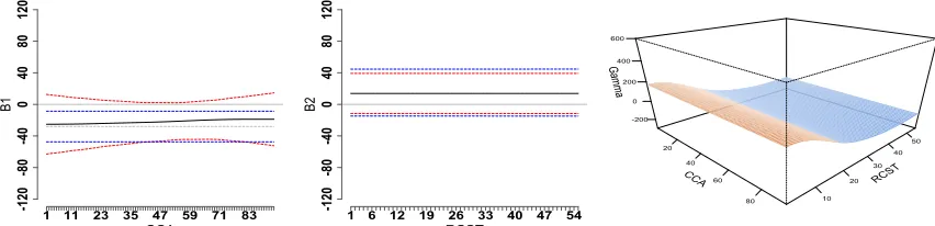
Figure A.2 displays the parameter estimates for the proposed interaction model fit from the
PFR framework. The CCA main effect estimates from the additive and interaction model are
highly similar. The additive model parameter fit has been shrunk to a negative constant. The interaction model estimated main effect for CCA is also negative, but has a slight upward slope,
and larger confidence bands that contain 0 across the domain of the tract. For the RCST, the
estimated main effects from the additive and interaction model are almost exactly the same; they have both been penalized to a constant positive value, whose magnitude is small such
that that the Bayesian confidence bands clearly contain 0. The interaction contour has been
completely flattened in the CCA direction, and slopes gently from positive to negative in the direction of the RCST. Nonetheless, all the points on the contour are not significant when
measured point-wise using the Bayesian confidence bands.
Figure A.3 displays the FPCR parameter estimates for the additive and interaction model. Noticeably, the FPCR estimates are more wiggly than those estimates from PFR; but overall the
results are qualitatively similar. The main effect estimates for CCA are both negative across the
tract domain, while the main effect estimates for RCST are positive near the beginning of the tract and then level to zero. The estimated interaction contour is highly similar qualitatively to
that fit with PFR, but more wiggly. The interaction contour is nearly flat in the CCA direction,
no coordinates on the contour are significant when measured point-wise using the Bayesian
confidence bands.
Based on these fits, is it advantageous to include an interaction effect in this model? The
Bayesian intervals for the estimated interaction contours suggest not. However to further aid
explanation, we use learning from our simulation experiment (see Section 2.5), and consider the average prediction error (APE) corresponding to both fitting approaches. Calculations give
average prediction error (APE) for the functional interaction model fit of 150.3 and APE =
154.2 for the additive model for FPCR the APEs were 150.2 and 155.0 for the interaction and additive models. Close estimates of the main effects, and similar APEs for the additive and
interaction models show support in favor of the lack of an interaction effect between the CCA
and RCST. Point-wise confidence bands, similarity of the main effect estimates, and prediction error are ad-hoc indicators of whether interaction is present in the model. The motivates our
work in Chapter 3, where we pursue formal hypothesis tests for the functional interaction effect.
2.6.2 Application to AneuRisk study
The second application of our method is to the AneuRisk65 data described in Sangalli et al.
(2009). The goal of this study is to identify the relationship between the geometry of the
internal carotid artery (ICA) and the presence or absence of an aneurysm on the ICA. The study contains a collection of 3D angiographic images taken from 65 subjects thought to be
affected by a cerebral aneurysm. Of these 65 subjects, 33 have an aneurysm located on the
internal carotid artery (ICA), 25 have an aneurysm not located on the ICA, and 7 have no aneurysm. Since the presence or absence of an aneurysm on the ICA is of primary of interest,
subjects in the latter two groups are combined. For each subject, the images are summarized
to describe the geometry of the ICA. Piccinelli et al. (2007) approximate the centerline of the artery in 3D space and estimate the corresponding width of the artery along this centerline in
terms maximum inscribed sphere radius (MISR). Sangalli et al. (2007) provide a measure of
curvature of the artery in 3D space along the artery centerline. The curvature and MISR profiles observed along the ICA centerline serve as our functional predictors. In this situation, the 3D
geometries of the arteries are more thoroughly described by the combination the curvature and
MISR values taken along the ICA centerline, and therefore it makes sense to include a two-way interaction term in the model. Our interest is to infer whether a including a two-way interaction
term between the curvature and MISR profiles helps better explain the presence or absence of an aneurysm on the ICA.
Before applying the proposed procedure we use the registration method described in Staicu