Copyright2000 by the Genetics Society of America
Maximum Likelihood Estimation of Recombination Rates From Population Data
Mary K. Kuhner, Jon Yamato and Joseph Felsenstein
Department of Genetics, University of Washington, Seattle, Washington 98195 Manuscript received December 3, 1999
Accepted for publication June 29, 2000
ABSTRACT
We describe a method for co-estimatingr⫽C/(whereCis the per-site recombination rate andis the per-site neutral mutation rate) and⌰ ⫽ 4Ne (where Ne is the effective population size) from a
population sample of molecular data. The technique is Metropolis-Hastings sampling: we explore a large number of possible reconstructions of the recombinant genealogy, weighting according to their posterior probability with regard to the data and working values of the parameters. Different relative rates of recombination at different locations can be accommodated if they are known from external evidence, but the algorithm cannot itself estimate rate differences. The estimates of⌰are accurate and apparently unbiased for a wide range of parameter values. However, when both⌰andrare relatively low, very long sequences are needed to estimateraccurately, and the estimates tend to be biased upward. We apply this method to data from the human lipoprotein lipase locus.
S
EQUENCES from loci that do not undergo recombi- over many different recombinant genealogies in propor-tion to each genealogy’s expected contribupropor-tion to the nation (for example, mammalian mitochondrialloci) have the same coalescent genealogy at every site. likelihood.
We have previously described similar methods for esti-In contrast, when recombination occurs adjacent sites
may have different, although correlated, genealogical mating ⌰ and for co-estimating ⌰ and exponential growth rate (Kuhner et al. 1995, 1998). The current histories. Reconstructing these genealogies with
cer-method is an extension of these, though it is more tainty is impossible. However, we can make inferences
complex because rearrangement of recombinant gene-about parameters such as population size and
recombi-alogies is more difficult. The basic method is maximum nation rate by considering a sample of plausible
geneal-likelihood estimation using Metropolis-Hastings sam-ogies.
pling (Metropoliset al.1953;Hastings1970) of candi-We can construct a structure, analogous to a
geneal-date genealogies. We sample genealogies on the basis ogy, which shows the ancestry of each site from a set
of their posterior probability with regard to the data at of sampled individuals. Unlike an ordinary coalescent
a trial value of the parameters and then use the sampled genealogy this is not necessarily a branching tree; its
genealogies to evaluate the relative likelihood of other general form is a directed graph, as described by
Hud-values of the parameters. This importance sampling
ap-son(1990). Such graphics have been called “ancestral
proach concentrates the sampled genealogies in regions recombination graphs” by Griffiths and Marjoram
of high posterior probability, which is much more effi-(1996); we use the phrase “recombinant genealogies”
cient than using random genealogies from the prior, to emphasize their logical similarity to genealogies.
Fig-and avoids the potential bias of using only a single gene-ure 1 shows a recombinant genealogy for a small case.
alogy reconstruction as in the UPBLUE method ofFu
A recombinant genealogy can provide information
(1994). about two parameters:⌰ ⫽4Ne, the product of
effec-Such an approach is especially useful in cases with tive population size and neutral mutation rate per site,
recombination, since the space to be sampled is larger andr⫽C/, the ratio between per-site recombination
(rendering random sampling particularly inefficient) rate and per-site mutation rate. If the genealogy were
and the chance of making a single genealogy reconstruc-known with certainty (including all of its branch
tion that is correct or nearly so is much smaller. lengths), we could make a maximum likelihood
esti-The sampler with recombination is useful both in mate of these parameters using a simple extension of
estimating the recombination rate itself and in allowing Kingman’s coalescent (Kingman1982a,b) as suggested
accurate estimation of other parameters from data con-byHudson(1990). Since the true genealogy is
unavail-taining recombinations. Attempting to estimate, for ex-able in practice, we estimate the parameters by sampling
ample,⌰in recombinant sequences using an approach that does not take recombination into account will lead to an overestimate (Kuhneret al.2000). Thus, in addi-Corresponding author:Mary K. Kuhner, Department of Genetics,
Uni-tion to its use in estimating recombinaUni-tion rate, this
versity of Washington, Box 357360, Seattle, WA 98195-7360.
E-mail: [email protected] algorithm opens the way for more precise use of nuclear
Figure1.—A recombinant geneal-ogy of four sequences, showing two recombination events dividing the genealogy into three subtrees.
gene sequences in assessing other population parame- considered: this is a requirement of the diffusion ap-ters. proximations used in the Kingman-Hudson coalescent. We are aware of at least two other likelihood-based When the algorithm is applied to DNA or RNA se-approaches to this problem.GriffithsandMarjoram quences or SNPs, a site is a single aligned column of (1996) describe a method that also uses importance base pairs. For future applications to microsatellite or sampling to estimate recombination rate on the basis electrophoretic data, a “site” is a single microsatellite of consideration of sampled genealogies, but using the locus or a single electrophoretic locus, and recombina-independent-sample algorithm developed byGriffiths tion is estimated between linked “sites.”
andTavare´(1993).Felsensteinet al.(1999) compare Definition of a recombinant genealogy:A nonrecom-the conceptual bases of nonrecom-these approaches. R. Nielsen binant coalescent genealogy is defined (Kingman
(unpublished results) describes a sampler somewhat 1982a,b) as just those lineages that contribute to the similar to ours, but in a Bayesian framework and without observed individuals. Several ways to extend this concept co-estimation of ⌰. Further work will be required to to a recombinant genealogy can be imagined. We compare the strengths and weaknesses of the different choose to define the recombinant genealogy of a sample approaches. as containing only lineages that contribute at least one site to the sample, and only recombinations that sepa-rate at least two sites contributed to the sample. Lineages
METHODS and recombinations that do not fulfill these criteria
will not leave any trace in the sampled sequences, and Parameters:Our approach estimates two parameters.
defining the genealogy to exclude them reduces its size, The first is⌰ ⫽4Ne, whereNeis the effective
popula-making it easier to analyze. tion size in individuals andis the mutation rate per
Further reductions in the size of the recombinant site per generation. The second isr⫽C/, whereCis
genealogy, without loss of information, are certainly the recombination rate per unit of intermarker distance
possible. We discuss one such reduction under “final per generation. In both cases,is present because we
coalescent tactic” below. Another reduction would be cannot directly observe time, only the occurrence of
to remove from consideration all recombinations that mutations. We assume that the relative distance between
are “loops”; that is, the two sequences that combine in markers is known. In the simple case of continuous
a recombination are nearest neighbors with no interven-DNA sequence, for example, all sites could be assumed
ing coalescences. Loops have no effect on the data and to be equally spaced. For single nucleotide
polymor-could therefore be discarded, but we have not yet phism (SNP) data known distances between SNP
mark-worked out the necessary adjustments to the prior prob-ers could be provided. We assume that multiple
recom-ability. binations do not occur simultaneously and therefore
genealogy sampler requires two terms, the probability of the data with respect to the genealogy [P(D|G)] and the probability of the genealogy with respect to the parameters [in this case,P(G|⌰,r)].
In the recombinant case, P(D|G) can be calculated straightforwardly for any of a large number of muta-tional models as long as the model assumes that sites are independent and therefore only the genealogy of a specific site is relevant to its likelihood. The indepen-dence assumption can be relaxed as long as the correla-tion between sites does not depend on the genealogy—
for example, adjacent sites can be allowed to have Figure2.—Eligible sites. Subgenealogies for sites 1–10 and 11–20 are shown. There is a single recombination event; sites autocorrelated rates.
1–10 are contributed by the right-hand sequence and sites Our implementation for nucleotide sequences is
11–20 by the left-hand one. On subtree A, sites 1–10 are not based on the one in PHYLIP (Felsenstein 1993). It
eligible for further recombination in the branch marked in uses the substitution model of Felsenstein as described gray because they do not pass through that branch to the tips; in Kishino and Hasegawa (1989), which allows un- similarly, on subtree B, sites 11–20 are not eligible on the gray branch. Such sites are not considered when calculating the equal nucleotide frequencies and differences between
probability of recombination. transition and transversion rate. Variation of rate among
sites, with possible autocorrelation, is accommodated by the Hidden Markov model of Felsenstein and
For such genealogies the Kingman-Hudson prior is
Churchill (1996). Other substitution models could easily be used instead.
P(G|⌰,r)⫽
冢
2⌰
冣
KrXexp冢
兺
i⫺
冤
ki(ki⫺1)⌰ ⫹ rsi
冥
t冣
,For SNP data we could use the same model, omitting autocorrelation (since SNP sites are usually widely
(1) spaced and correlation between adjacent sites seems
unlikely) and applying a correction to the termP(D|G), where K is the total number of coalescences in that accounting for the method by which the SNPs were genealogy,Xis the total number of recombinations,i ascertained (Kuhneret al.2000). is the number of the time interval,k
iis the number of
We assume that the mutational model parameters lineages in interval i, and s
i is the weighted sum of
(such as transition/transversion ratio and nucleotide eligible links in interval i, weighting each link by its frequencies) are known. Experience with phylogeny es- length.
timations suggests that maximum likelihood methods This can be understood as the product of three types are fairly robust to errors in specification of the muta- of terms: the probability density 2/⌰of a specific coales-tional model (see, for example,Fukami-Kobayashiand cence, the probability densityrof a specific
recombina-Tateno1991). tion, and the probability exp(⫺ (k(k⫺1)/⌰ ⫹ rs)/t) The prior probability of the genealogy,P(G|⌰,r), is an of the waiting time until the next event.
extension of Kingman’s coalescent (Kingman1982a,b) Overview of procedure:The Metropolis-Hastings ge-developed byHudson(1990). The genealogy is consid- nealogy sampler that we originally derived for nonre-ered as a series of time intervals, starting at the tips; combinant sequences (Kuhneret al.1995, 1998) works each time interval is bounded by an event (either recom- by a two-phase process. It begins with an initial geneal-bination or coalescence). The rate of coalescence is⌰/ ogy and an initial value of the parameters: in the simplest [k(k⫺ 1)], where kis the number of lineages in that case, the single parameter⌰, whose initial value is called time interval. The rate of recombination isrs, where s ⌰
0. In the first phase, a new genealogy is created by
is the length of the region in which a recombination locally rearranging the previous genealogy in propor-could occur, summed over allklineages. tion to the coalescent prior probabilityP(G|⌰
0) (given
Since we have defined the recombinant genealogy to byKingman1982a,b). In the second phase, this geneal-include only recombinations that separate two or more ogy is accepted or rejected based onP(D|G), the proba-sites destined to contribute to the observed data, we bility of the sequence data on the genealogy (given by must count as potential locations for recombination Felsenstein1981). Repetition of this process, which is only those inter-site links that would produce such a equivalent to sampling from the posterior probability recombination. Thus, only a subset of inter-site links, P(G|⌰
0)P(D|G), produces a set of genealogies from
called “eligible links,” are counted in calculating the which a maximum likelihood of ⌰can be made. For probability of recombination. Figure 2 shows an exam- the case without recombination the relative likelihood ple: if a region is destined to be replaced, higher up in becomes
the genealogy, with a different sequence, we do not
allow any recombinations within it, since they would L(⌰)
L(⌰0)
≈1
n
兺
iP(Gi|⌰)
P(Gi|⌰0)
(Kuhneret al. 1995). This estimator is most efficient estimate the maximum likelihood value of⌰. Otherwise we co-estimate the maximum forrand⌰.
when ⌰0 is close to its maximum likelihood estimate
(MLE), so it is useful to run several iterations of the Multiple loci:If information from multiple unlinked regions of the genome is available, an overall estimate sampler, using the estimated⌰of each iteration as the
starting⌰0of the next. of the parameters can be made by multiplying together
the regional likelihood curves, as long as any differences The local rearrangement scheme that was successful
for nonrecombinant genealogies (Kuhner et al.1995, in the values of the parameters are assumed to be known (for example, haploid and diploid data could be com-1998) cannot be directly adapted to recombinant
gene-alogies. It confines each rearrangement strictly within bined, using a factor of two difference in the value of Ne). Our previous samplers have been much more a local neighborhood in the genealogy, whereas in
re-combinant genealogies any lineage can interact with efficient with multiple unlinked loci than with a single locus, but we do not expect that to be the case here, any other. Instead, we adopt a more drastic form of
rearrangement: a lineage is broken at random, all lines since a single lengthy region with recombination com-bines the advantages of multiple loci (i.e., multiple site leading rootward from that lineage into the rest of the
genealogy are erased, and then the broken lineage is genealogies) with maximum ability to detect recombina-tions.
resimulated from the breakpoint downward toward the root, choosing events based onP(G|⌰0,r0) conditional
on the structure of the nonerased tree, until all resulting
IMPLEMENTATION lineages have coalesced. This approach was originally
This section discusses the details of the genealogy-developed by Beerli andFelsenstein(1999) for use
rearrangement process. Throughout, “down” is toward in the sampler with migration. Some additional
com-the root of com-the genealogy. plexity is needed in the sampler with recombination;
The objective is to erase and redraw a portion of this is discussed in theimplementationsection.
the genealogy in accordance with several goals. New Multiple chains:The importance sampling approach
genealogies should be produced in proportion to used in this sampler is most effective when ⌰0 and r0
P(G|⌰,r) to the extent that this is possible. Any devia-are near their MLEs. For this reason, it is useful to do
tions from this proportion must be matched with a com-a series of short chcom-ains, beginning ecom-ach run with the
pensating Hastings term (Hastings1970). For the Mar-maximum likelihood estimates of ⌰ and r from the
kov chain to work properly, there must be no irreversible previous chain. Because the algorithm with
recombina-steps; if the process can go from genealogy A to geneal-tion rejects a higher proporgeneal-tion of genealogies and is
ogy B in one step, it must be able to go from B to A in searching a higher-dimensional space, the short chains
one step as well. Finally, for the sampler to be efficient must be longer than for the nonrecombinant sampler.
it is desirable not to change the genealogy too much in This procedure must be modified if the estimate of
one step, or the new genealogy will probably be rejected.
rfrom a given chain is 0. Since genealogies generated
We begin by choosing one branch of the genealogy, withr0⫽0 will never contain recombinations, and
analy-other than the root branch, at random. This branch sis of Equation 1 shows that a set of genealogies
con-is erased, as are all recombinations rootward of and taining no recombinations will always return r ⫽ 0, 0
dependent on it. The branch is then resimulated down-represents an absorbing state that the process can never
ward according to a conditional recombinant-coales-leave once it is reached. We have experimented with
cent prior until all lineages are once again attached settingrto a small positive value (data not shown) but
to the genealogy. This resimulation includes a rate of it is difficult to choose an appropriate value. Instead we
recombination (a lineage being simulated splits into use an approach developed byBeerliandFelsenstein
two lineages, each containing a subset of the sites) and (1999) in which we add one recombination to the final
a rate of coalescence (a lineage under simulation co-genealogy of each chain that would otherwise have
alesces either with another lineage under simulation or none, except for the final chain. This prevents the “fatal
with a lineage already in the tree). attraction” ofrto 0 and seems to minimize interference
Lineages being resimulated are called “active” lin-in the process, slin-ince addlin-ing a slin-ingle recomblin-ination
eages, and lineages in the remainder of the genealogy represents the least possible unit of change in the
esti-are “inactive” lineages. mate. We do not introduce an arbitrary recombination
Resimulation downward involves drawing a waiting into the final chain, so the biasing effect of this
correc-time until the next event (using the Kingman-Hudson tion is limited to its influence on the final chain’s r0
prior) and then checking to see if that time falls within value.
the current time interval. If it does, an event is added Construction of likelihood curve:At intervals,
geneal-to the genealogy, and the process is repeated for the ogies are sampled from the Markov process for use in
new time interval just below the added event. If it does constructing a likelihood curve. When there are no
re-not, the process proceeds down to the next time interval combinations in any of the sampled genealogies, the
This procedure can create a new genealogy that is
Prob(rec)⫽
兺
j
rsj⫹
兺
krsk. (4)
outside the defined state space of legal genealogies. A rearrangement in the upper part of the genealogy can
The waiting time formula is then render an existing branch lower down meaningless—it
no longer contributes any sites to the tips. For example,
time⫽ log(U)
Prob(coal)⫹Prob(rec), (5) imagine a branch whose only contribution is to supply
site 1 to tip 7. A recombination is now added higher in
whereUis a random number chosen uniformly between the tree that supplies site 1 to tip 7 from a different
0 and 1. lineage. The original branch now has no sites to
con-The only step in the rearrangement process that is tribute.
not driven by the coalescent prior probability is the Since we define recombinant genealogies as having
decision where to make the initial cut. This algorithm no such branches, it is tempting to reject such
re-is an example of a “reversible jump MCMC” (Green
arrangements, but doing so would mean that all
re-1995) in that it moves among state spaces with different arrangements of the upper parts of highly recombinant
dimensionality (in this case, numbers of branches, since trees would tend to be rejected, preventing the sampler
each recombination adds two branches to the geneal-from mixing well.
ogy). As Green points out, care must be taken to pre-It is also tempting to simply prune out meaningless
serve detailed balance when making transitions between branches as they arise, but this violates the reversibility
states of different dimension. of the Markov chain. If we make a change and prune
We choose the branch to be cut uniformly among all out a lower branch, reversing the change would require
branches except the root. This creates an imbalance “pruning in” the missing branch. To preserve
reversibil-between forward and reverse transitions that change ity, if we are going to remove a branch when all its
the number of branches, because the more branches a meaningful sites have been taken from it, we must be
genealogy has, the less likely it is that the specific branch prepared to add a branch when new meaningful sites needed to make the reverse change will be chosen. become available during the rearrangement process. Thus, a move from a specific genealogy with fewer re-This is done by keeping a record of which links were combinations to a specific genealogy with more recom-meaningful in each branch of the old genealogy. Con- binations has a higher probability than the reverse struction of the new genealogy occurs from the tips move. To restore balance we introduce a Hastings term downward, time interval by time interval. For each time (Hastings 1970) representing the ratio of forward to interval, each inactive branch is checked to see whether back transition. Our probability of acceptance is de-it contains links newly made meaningful by the ongoing cided on the basis of the formula
rearrangements. If it does, evaluation of the interval
includes the possibility that a new recombination may Prob(accept)⫽P(D|Gnew)
P(D|Gold)
Qnew
Qold, (6)
occur at one of the newly meaningful links. At the end
of the rearrangement process, the genealogy is checked where Q is the reciprocal of the number of branches for meaningless branches and they are removed. This in that genealogy, excluding the root. If Prob(accept) process is fully reversible and preserves the desired sam- isⱖ1 the new genealogy is always accepted; otherwise pling fromP(G|⌰,r). it is accepted with that probability.
These new recombinations can be thought of as “hid- Recombinations near the rootward end of the geneal-den passages”: conceptually they are always present, but ogy may find themselves below the root after a re-they reveal their presence only when, due to re- arrangement; such structures are removed from the ge-arrangements elsewhere, they have an influence on the nealogy when encountered, since they are not part of descent of sites to the sampled individuals. We do not our definition of a recombinant genealogy. To avoid attempt to keep track of previous hidden passages but irreversibility, once the resimulation process is below instead regenerate them when they are needed (in other the level of the old root, it is necessary to resimulate words, when a rearrangement elsewhere in the geneal- the root lineage as well as the other lineages, since its ogy has made formerly meaningless recombinations recombinations have been stripped out and must be meaningful). replaced. This is a specialized case of the hidden pas-The probabilities work out as follows. pas-The active lin- sages issue: recombinations on the root are “hidden” and must be revealed when that branch is no longer eages are denoted j and the inactive ones k. Then, sj
the root. are the meaningful links on active lineagejandskare
One problem encountered in practical testing is that the (newly) meaningful links on inactive lineage k,
for high values ofr, the number of recombinations in weighted in each case by the length of each link:
the sampled genealogies varies widely and may become very large. Such large genealogies present the risk of Prob(coal)⫽k(k⫺1)⫹2jk
program unacceptably. An upper limit may be placed only 2001 sites because data sets with 1001 sites were often invariant. For ⌰ ⫽ 0.1 we used 1001 sites and on the allowable number of recombinations, but the
estimate will be biased downward if this limit is encoun- 1501 sites because with 2001 sites we encountered the limits of computer memory at the higher recombination tered too frequently.
To increase the practical usefulness of the method, values; we also omittedr⫽0.08 for this case.
For each parameter combination, we simulated 100 it is possible to define as “uninteresting” any
recombina-tion involving only sites that have completed coalesc- genealogies. Initial values of⌰were estimated using the method of Watterson (1975). The initial value of r
ing—that is, sites of which only one copy is present in
the genealogy at the point of the contemplated recombi- was arbitrarily set to 0.01. A random nonrecombinant genealogy was used as the starting genealogy. RECOM-nation. This method was proposed to us by Richard
Hudson (personal communication). Recombinations BINE executed five short chains of 20,000 re-arrangements each followed by two long chains of involving such sites can never change the value of
P(D|G), so they represent bookkeeping overhead with 50,000 rearrangements each, sampling every 20th gene-alogy.
no informational value. Conceptually simple changes
to the rearrangement process and to the evaluation of Example data set:To observe the performance of the method on biological data we used human lipoprotein the prior can eliminate such recombinations. However,
these changes are expensive in terms of computer time lipase (LPL) data (Clark et al.1998;Nickersonet al.
1998), which consist of 9734 bp of intron and exon data and space and are only worth using for high values ofr.
In such cases they reduce the number of recombinations from 71 individuals (142 chromosomes) derived from three populations: African Americans from Mississippi, greatly and therefore allow for a more memory-efficient
estimate, and possibly a faster one. We refer to this tactic Finns from North Karelia, Finland, and non-Hispanic Whites from Minnesota. We considered only nucleotide as the “final coalescence” criterion because it eliminates
each site from consideration as that site reaches its final substitution differences, disregarding insertion/dele-tion mutainsertion/dele-tions, and we omitted the 20 rare variable sites coalescence. Use of the final coalescence criterion
should not have any systematic effect on the program’s (rare allele present in only one or two copies) for which Clark’s group did not determine phase.
results.
Convergence:Results from a sampler of this type are In this analysis we used a transition/transversion ratio of 1.4 based on the ratio of visible transitions to transver-valid only if the sampler has adequately searched the
space of genealogies. As with most Metropolis-Hastings sions in the full data. We calculated base frequencies on the basis of the polymorphic sites only, and in the samplers, we do not have an exact test to determine
when the sampler has run long enough. Several heuris- subpopulation analyses we used the frequencies from the corresponding subpopulation. We used two rate tics, however, can help users of the method decide if
they are making a large enough sample. Results from categories with a ratio of 1:0.75 and prior probabilities of 9:1, based on the Nickersonet al.(1998) estimate the preliminary short chains should stabilize around a
value: if each short chain produces a higher (or lower) that 90% of the sequence was noncoding and that the rate in coding regions was 75% of that in noncoding estimate of the parameters than the one before, the
process has not reached equilibrium. Results from sev- regions. We analyzed only the polymorphic sites using the “reconstituted DNA” SNP model of Kuhner et al.
eral runs with different initial parameters should
con-verge on similar values. For the simulations, we experi- (2000) in which sites not noted were assumed to be invariant sites of unknown nucleotide; this was more mented with different initial values and feel that the
given results represent an adequate (although not gen- convenient than analyzing the full DNA sequence and is expected to give similar results.
erous) sampling of the search space.
Simulation testing:To test the accuracy of the method We analyzed each subpopulation separately using the following strategy: 10 short chains of 50,000 steps and we simulated recombinant genealogies of 10 individuals
using a program provided by Richard Hudson (per- 1 long chain of 1,000,000 steps. Each chain had a burn-in period of 1000 steps and was subsequently sampled sonal communication). This program generates
inde-pendent random genealogies according to the King- every 20th step. We used the Watterson(1975) esti-mate of⌰as our starting point for⌰and 0.05 as our man-Hudson prior. For each genealogy we simulated
DNA data using the same mutational model used by starting point forr.For the combined data we doubled the length of all chains (to 100,000 and 2,000,000 steps, our algorithm. All links were 1 unit long, as would be
the case for contiguous nucleotide sequence data. respectively) to reflect the larger search space of the full data.
We simulated data under several values of⌰(0.005, 0.01, and 0.1) and r(0, 0.02, 0.04, and 0.08). In most cases we used sequences of length 1001 and 2001. (We
RESULTS chose these numbers because a sequence of length 1001
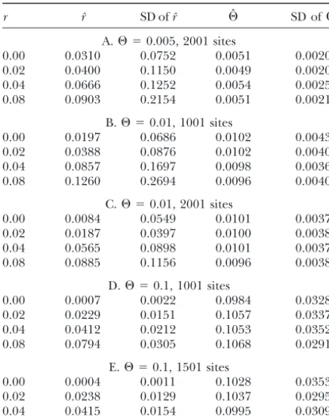
TABLE 1 formative sites (polymorphic sites present in more than one individual). The estimates forr⫽0 are particularly
Simulation results
poor because such troublesome cases arise from under-lying genealogies that are, by chance, unusually short.
r rˆ SD ofrˆ ⌰ˆ SD of⌰ˆ
It is more likely for the single genealogy produced in A.⌰ ⫽0.005, 2001 sites a case without recombination to be unusually short than
0.00 0.0310 0.0752 0.0051 0.0020
for a collection of recombinant subgenealogies to be
0.02 0.0400 0.1150 0.0049 0.0020
unusually short across the entire sequence. By this
rea-0.04 0.0666 0.1252 0.0054 0.0025
soning, the best way to improve the accuracy of
estima-0.08 0.0903 0.2154 0.0051 0.0021
tion when⌰ and r are low should be to increase the B.⌰ ⫽0.01, 1001 sites
number of base pairs surveyed. Indeed, doubling the
0.00 0.0197 0.0686 0.0102 0.0043
sequence length from 1001 to 2001 bp produced
sub-0.02 0.0388 0.0876 0.0102 0.0040
stantial improvement in the estimate (compare Table
0.04 0.0857 0.1697 0.0098 0.0036
0.08 0.1260 0.2694 0.0096 0.0040 1B with 1C).
Our artificial addition of one recombination to each C.⌰ ⫽0.01, 2001 sites
chain when there would otherwise be none could also
0.00 0.0084 0.0549 0.0101 0.0037
0.02 0.0187 0.0397 0.0100 0.0038 contribute to an upward bias in the estimate ofr; how-0.04 0.0565 0.0898 0.0101 0.0037 ever, if this correction is not made the results are only 0.08 0.0885 0.1156 0.0096 0.0038 slightly lower (data not shown) so we do not believe
this to be a major effect. D.⌰ ⫽0.1, 1001 sites
0.00 0.0007 0.0022 0.0984 0.0328 As a case study we present an analysis of the human 0.02 0.0229 0.0151 0.1057 0.0337 LPL data ofClark et al. (1998) and Nickersonet al. 0.04 0.0412 0.0212 0.1053 0.0352 (1998). These data consist of sequences of length 9734
0.08 0.0794 0.0305 0.1068 0.0291
bp from 71 individuals sampled from three populations E.⌰ ⫽0.1, 1501 sites (African Americans from Mississippi, Finns from North 0.00 0.0004 0.0011 0.1028 0.0353 Karelia, and non-Hispanic Whites from Minnesota). 0.02 0.0238 0.0129 0.1037 0.0295 These data show visible evidence of recombination and
0.04 0.0415 0.0154 0.0995 0.0309
it is thus interesting to assess them with RECOMBINE. Means and standard deviations of parameter estimates from However, it should be noted that one of the program’s 100 simulated data sets of 10 sequences each. Presented as key assumptions (a single nonsubdivided population) truer, mean estimate of r, standard deviation ofr, estimate is clearly violated by these data whether they are ana-of⌰, and standard deviation of⌰. The majority of replicates
lyzed as one large population or three smaller ones. A were calculated without the “final coalescence” criterion, but
more correct analysis would require combining the logic it was used in specific cases where the program would
other-wise have run out of space and throughout the subtables with of MIGRATE (BeerliandFelsenstein1999) with RE-⌰ ⫽0.1. COMBINE, a project we are currently undertaking.
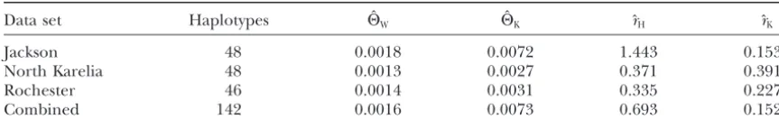
We analyzed the three population data sets separately and together; results are shown in Table 2, with esti-Table 1. For all of the values of⌰examined, estimation mates of ⌰ using the method of Watterson (1975) of⌰showed little or no bias and good accuracy. The and ofrusing the method ofHudson(1987) repeated results with⌰ ⫽0.01 and 1001 bp can be compared with fromClark et al.(1998) for comparison.
results from the nonrecombinant sampler COALESCE (Kuhneret al.1995). The standard deviations are very
similar, suggesting that little power is lost by estimating DISCUSSION
⌰in the presence of recombination. This confirms
pre-The method described here is able to recover⌰and vious findings ofHudson(1983) for pairwise estimators
rwith good accuracy in many cases and appears to have of⌰.
practical advantages over existing pairwise methods. It When the true value of ⌰ was relatively low, a
pro-avoids the bias seen when a nonrecombinant sampler nounced upward bias in the estimaterˆwas seen (Table
is used on recombinant data (Kuhneret al.2000). The 1, A–C), particularly when r was also low. In contrast,
computational burden is not excessive: for example, for relatively high values of⌰we recovered good
esti-each of the single-population LPL runs tookⵑ4 hr on mates ofr(Table 1, D and E).
a 500-MHz Alpha workstation. The estimates ofrfrom the low-⌰cases are a mix of
Several points are noteworthy in the analysis of the many values near zero and a small population of high
LPL data. In general, RECOMBINE gives somewhat values associated with likelihood surfaces that are nearly
higher estimates of⌰and lower estimates ofrthan the flat (data not shown). These flat likelihood surfaces
pairwise methods. It may be better able than the pairwise come from data sets that are nearly uninformative for
TABLE 2
Analysis of LPL sequences
Data set Haplotypes HˆW HˆK ˆrH rˆK
Jackson 48 0.0018 0.0072 1.443 0.1531
North Karelia 48 0.0013 0.0027 0.371 0.3910
Rochester 46 0.0014 0.0031 0.335 0.2273
Combined 142 0.0016 0.0073 0.693 0.1521
Results for a human lipoprotein lipase data set (Clarket al.1998;Nickersonet al. 1998). Shown are the number of haplotypes in each section of the data set, Hˆ from Watterson’s (1975) estimator (HW) and
RECOMBINE (HK), andˆ fromr Hudson’s (1987) estimator (rH) and RECOMBINE (rK). Non-RECOMBINE
results are taken fromClarket al.(1998) with permission.
caused by recurrent mutation and site inconsistencies 1999). By contrast, in data containing recombinations maximal efficiency is obtained by having a single locus caused by recombination.
The Watterson (1975) estimator of ⌰ gives very with long sequences. This captures some of the advan-tages of multiple loci, since recombination implies dif-similar values for all subpopulations, whereas
RECOM-BINE suggests that the Jackson (African-American) sam- ferent subgenealogies for different parts of the loci, and the use of continuous sequence maximizes the algo-ple and the combined data reflect a larger population
than the two European samples. This is consistent with rithm’s ability to detect recombinations.
A number of extensions to the method described here many observations of higher diversity in Africans and
also with the possibility of admixture in the African- are possible. It could be combined with the population-growth estimator of FLUCTUATE (Kuhneret al.1998) American population. The homogeneous Watterson
re-sults reflect the fact that number of variable sites (the or the migration-rate estimator of MIGRATE (Beerli
andFelsenstein1999) to allow analysis of more com-only information used by Watterson’s estimator) does
not vary much among the populations even though plex population structures. Gene conversion could be added as a supplement to conventional recombination, overall haplotype diversity is noticeably higher in the
Jackson population. RECOMBINE makes fuller use of given an appropriate probability model for conversions. Any form of data for which map information is avail-the available information.
Hudson’s (1987) estimator gives a particularly high able and for which a data likelihood model can be developed, such as microsatellite data, electrophoretic value ofr for the Jackson population, butClarket al.
(1998) suggest that this is due to the greater diversity allele data, or restriction site data, can in principle be used to infer recombination rate.
of the Jackson sample, which provides greater detection
power. RECOMBINE, in contrast, does not suggest a The ability to sample clouds of recombinant genealo-gies can be used for maximum likelihood linkage dis-higher recombination rate for the Jackson sample. Since
RECOMBINE can consider recombinations even in re- equilibrium gene mapping by computing the probabil-ity of the observed pattern of a disease trait on the gions where the data are uninformative, rather than
inferring recombination only where enough variability various genealogies under different hypotheses for the disease gene location (M. K. Kuhner and J.
Felsen-exists to reveal it, we would expect it not to be misled
by differences in polymorphism level. stein, unpublished results).
The program could provide its user with the cloud A few general conclusions about study design are
pos-sible. To estimate the recombination parameterraccu- of sampled genealogies, but this is difficult to compre-hend. It would be desirable to combine information rately with a sample of 10 individuals, for most
organ-isms it will be necessary to examine tens of thousands about the cloud into a summary genealogy analogous to a consensus tree. However, it is not obvious how to of base pairs. Adding more individuals will be only
mod-estly helpful, since most of the new individuals will be make a consensus of recombinant genealogies. At the moment, only basic summary information, such as the closely related to individuals already in the sample and
therefore provide little additional genealogical struc- distribution of number of recombinations or of recom-bination breakpoints, can be collected.
ture. The computational burden of long sequences
could be reduced by use of SNPs or some other type of A final addition that would improve the usefulness of the program would be to attempt an estimate of the marker rather than full DNA sequences, at some cost
in efficiency (Kuhneret al.2000). location of recombination “hot spots” and “cold spots.” In theory this could be done by incorporating a Hidden Metropolis-Hastings samplers for nonrecombining
data are known to be more effective and less biased if Markov model (HMM) of recombination frequency into the sampler itself, analogously with the use of an HMM multiple unlinked loci, rather than a single locus, are
Felsen-Lecture Notes-Monograph Series, Vol. 33), edited byF. Seillier.
steinandChurchill1996). A simpler approximation
Institute of Mathematical Statistics, Hayward, CA.
would be to use the HMM after the fact, in analysis of the Fu, Y.-X.,1994 A phylogenetic estimator of effective population size
or mutation rate. Genetics136:685–692.
sampled trees, to produce an estimate of the posterior
Fukami-Kobayashi, K.,andY. Tateno,1991 Robustness of
maxi-probability that specific intersite links are in one or
mum likelihood tree estimation against different patterns of base
another recombination rate category. substitution. J. Mol. Evol.32:79–91.
Green, P. J.,1995 Reversible jump Markov chain Monte Carlo
com-Availability of software: The Metropolis-Hastings
putation and Bayesian model determination. Biometrika82:711–
Monte Carlo algorithm described here is available from 732.
the authors as program RECOMBINE in the package Griffiths, R. C.,andP. Marjoram,1996 Ancestral inference from samples of DNA sequences with recombination. J. Comput. Biol.
LAMARC, which uses an input/output format similar
3:479–502.
to the PHYLIP package. The program is written in C Griffiths, R. C.,andS. Tavare´,1993 Sampling theory for neutral and can be obtained by anonymous ftp fromevolution. alleles in a varying environment. Proc. R. Soc. Lond. Ser. B344:
403–410.
genetics.washington.edu in directory pub/lamarc or via
Hastings, W. K.,1970 Monte Carlo sampling methods using Markov
the World Wide Web at http://evolution.genetics. chains and their applications. Biometrika57:97–109.
Hudson, R. R.,1983 Properties of a neutral allele model with
intra-washington.edu/lamarc.html.
genic recombination. Theor. Popul. Biol.23:183–201. We thank Gary Churchill for pointing out the need for a Hastings Hudson, R. R.,1987 Estimating the recombination parameter of a ratio and Peter Beerli for extensive help in finding the maxima of finite population without selection. Genet. Res.50:245–250.
Hudson, R. R.,1990 Gene genealogies and the coalescent process, surfaces. We thank Richard Hudson for providing the recombinant
pp. 1–44 inOxford Surveys in Evolutionary Biology, Vol. 7, edited genealogy simulation program and helping us interpret its results,
by D. Futuymaand J. Antonovics. Oxford University Press, and for suggesting the final coalescence tactic. This research was
Oxford. supported by National Science Foundation grants BSR-8918333 and
Kingman, J. F. C.,1982a The coalescent. Stochastic Process. Appl. DEB-9207558 and National Institutes of Health grant 2-R55GM41716- 13:235–248.
04 (all to J.F.). Kingman, J. F. C.,1982b On the genealogy of large populations. J. Appl. Probab.19A:27–43.
Kishino, H.,andM. Hasegawa,1989 Evaluation of the maximum likelihood estimate of the evolutionary tree topologies from DNA sequence data, and the branching order in Hominoidea. J. Mol.
LITERATURE CITED
Evol.31:151–160.
Kuhner, M., J. YamatoandJ. Felsenstein,1995 Estimating
effec-Beerli, P.,andJ. Felsenstein,1999 Maximum likelihood
estima-tive population size and mutation rate from sequence data using tion of migration rates and effective population numbers in two
Metropolis-Hastings sampling. Genetics140:1421–1430. populations using a coalescent approach. Genetics152:763–773.
Kuhner, M. K., J. YamatoandJ. Felsenstein,1998 Maximum
likeli-Clark, A. G., K. M. Weiss, D. A. Nickerson, S. L. Taylor, A.
hood estimation of population growth rates based on coalescent.
Buchananet al., 1998 Haplotype structure and population
ge-Genetics149:429–434. netic inferences from nucleotide-sequence variation in human
Kuhner, M. K., P. Beerli, J. YamatoandJ. Felsenstein,2000 Use-lipoprotein lipase. Am. J. Hum. Genet.63:595–612.
fulness of single nucleotide polymorphism (SNP) data for
estimat-Felsenstein, J.,1981 Evolutionary trees from DNA sequences: a
ing population parameters. Genetics156:439–447. maximum likelihood approach. J. Mol. Evol.17:368–376.
Metropolis, N., A. W. Rosenbluth, M. N. Rosenbluth, A. H. Felsenstein, J.,1993 Phylip(Phylogeny Inference Package)
ver-TellerandE. Teller,1953 Equations of state calculations by sion 3.5c. Distributed by the author. Department of Genetics, fast computing machines. J. Chem. Phys.21:1087–1092. University of Washington, Seattle. http://evolution.genetics.
Nickerson, D. A., S. L. Taylor, K. M. Weiss, A. G. Clark, R. G.
washington.edu/phylip.html. Hutchinson et al., 1998 DNA sequence diversity in a 9.7-kb
Felsenstein, J., and G. A. Churchill, 1996 A hidden Markov region of the human lipoprotein lipase gene. Nat. Genet. 19: model approach to variation among sites in rates of evolution. 233–240.
Mol. Biol. Evol.13:93–104. Watterson, G. A.,1975 On the number of segregating sites in
Felsenstein, J., M. K. Kuhner, J. YamatoandP. Beerli,1999 Like- genetical models without recombination. Theor. Popul. Biol.7: lihoods on coalescents: a Monte Carlo sampling approach to 256–276.
inferring parameters from population samples of molecular data,