Isolation by distance in a quantitative trait.

(1)

Isolation

by

Distance in a Quantitative Trait

Russell Lande’

Department of Ecology and Evolution, University of Chicago, Chicago, Illinois 60637

Manuscript received July 6, 1990

Accepted for publication February 13, 1991

ABSTRACT

Random genetic drift in a quantitative character is modeled for a population with a continuous spatial distribution in an infinite habitat of one or two dimensions. The analysis extends Wright’s concept of neighborhood size to spatially autocorrelated sampling variation in the expected phenotype at different locations. Weak stabilizing selection is assumed to operate toward the same optimum phenotype in every locality, and the distribution of dispersal distances from parent to offspring is a (radially) symmetric function. The equilibrium pattern of geographic variation in the expected local phenotype depends on the neighborhood size, the genetic variance within neighborhoods, and the strength of selection, but is nearly independent of the form of the dispersal function. With all else equal, geographic variance is smaller in a two-dimensional habitat than in one dimension, and the covariance between expected local phenotypes decreases more rapidly with the distance separating them in two dimensions than in one. The equilibrium geographic variance is less than the phenotypic variance within localities, unless the neighborhood size is small and selection is extremely weak, especially in two dimensions. Nevertheless, dispersal of geographic variance created by random genetic drift is an important mechanism maintaining genetic variance within local populations. For a Gaussian dispersal function it is shown that, even with a small neighborhood size, a population in a two-dimensional habitat can maintain within neighborhoods most of the genetic variance that would occur in an infinite panmictic population.

T

HEORETICAL analysis of random genetic drift and local gene frequency differentiation in a population with a continuous spatial distribution was initiated by WRIGHT (1 943, 1946, 195 1) and MALE- COT (1948, 1967, 1969). WRIGHT described the stochastic equilibrium of geographic variation in terms of inbreeding coefficients ( F statistics) as a function of the geographic distance between local populations or neighborhoods. MALECOT derived the genetic relationship between individuals separated by a given distance in terms of the probability of identity by descent of their alleles. This work stimulated much empirical research on dispersal patterns, the effective sizes of local populations, and the geographic patterns of genetic variation [reviewed by WRIGHT (1978, Ch. 2), BARROWCLOUCH (1980) and CHEPKO-SADE et al. ( 1 987)], as well as further theoretical studies of random genetic drift in spatially structured populations (reviewed by NAGYLAKI 1989).

T h e present paper analyzes random genetic drift and phenotypic differentiation in quantitative characters for populations that are continuously distributed in space, based on methods developed by MA-

LECOT

( 1 967, 1969). I derive the geographic variance in the expected local phenotype, and the covariance between the expected phenotypes at different locali-

ties as a function of the distance between them in a one- or two-dimensional habitat of infinite extent. The form of the distribution of individual dispersal distances differs among species, but is usually leptokurtic

[ W R I G H T ( ~ ~ ~ ~ , Ch. 12; 1978, Ch. 2); T A Y L O R ( ~ ~ ~ ~ , 1980); SHIELDS (1982, Ch. 2); CHEPKO-SADE et al.

(1 987)]. Patterns of geographic variation and the decay of geographic covariance with distance are therefore analyzed for an arbitrary (radially) symmetric dispersal function which, for simplicity, is assumed to be homogeneous in space. For the special case of Gaussian dispersal, I investigate also the maintenance of genetic variability within local populations.

Serious difficulties have been encountered in the description of random genetic drift in spatially continuous models derived by a limiting process from two- dimensional discrete “stepping-stone” models (NAGY- LAKI 1989; ROUHANI and BARTON 1987). Such models yield impossible probabilities of identity by descent (approaching infinity) for small distances. Here I de- scribe random genetic drift in a continuous habitat as a spatially autocorrelated stochastic process determined by the dispersal function and the neighborhood size. Density-dependent regulation of local populations is postulated to maintain a nearly uniform population density in space. T h e present model, like that

’

Present address: Department of Biology, University of Oregon, Eugene, of MALECOT (1969), is therefore an approximation, Oregon 97403. because most mechanisms of density-dependence en-

(2)

tail that the dispersal function can not be strictly homogeneous in space (FELSENSTEIN 1975; SUDBURY 1977; KINGMAN 1977).

T H E MODEL

Random genetic drift in a single population: As- sume that the population is diploid, mates randomly and has discrete, nonoverlapping generations. T h e distribution of a quantitative character, z, in a randomly mating population is often approximately nor- mal (Gaussian) at least on an appropriate scale of measurement [WRIGHT (1968, Ch. 11); FALCONER

( 1 98 1, Ch.

17)].

Let Z, denote the mean phenotype in generation t , measured before selection and reproduction. T h e total phenotypic variance, a‘ = V,

+

V,, is the sum of the additive genetic variance, V,, and the environmental variance (including nonadditive genetic variance), V,. T h e heritability of the character is h‘ = V,/u2. If the effective population size, N , is greater than a few dozen individuals and multiple (unlinked) loci contribute to the additive genetic variance, V, can be considered roughly constant [BULMER (1985, Ch. 12)]. Weak stabilizing selection toward an optimum phenotype, arbitrarily set at zero, can be approximated by assigning to individuals with phenotype z a fitness W(z) proportional to the Gaussian function

W( z) = exp{-z2/2w2]. (1)

T h e evolutionary dynamics of the mean phenotype under the joint action of stabilizing selection and random genetic drift can then be approximated by the stochastic difference equation (LANDE 1976; Rou-

HAM and BARTON 1987)

;,+I = (1

-

s)Z*

+

E , (2)

in which s = Vg/Vs with V, = w2

+

u2 E w2

+

V,, where the approximation is accurate under weak selection. E , is a noise term with mean zero, variance

Vg/N and no temporal autocorrelation. Starting from a given initial mean phenotype at generation 0, the probability distribution of the mean phenotype in later generations is Gaussian. After about 1/(2s) generations the variance in the mean phenotype caused by random genetic drift approaches the equilibrium value VJ(2N) = Vg/(2Ns) (LANDE 1976).

As we shall see, the spatial structure of a population drastically alters the balance between random genetic drift and stabilizing selection. Before analyzing spatially structured populations, let us first review and extend WRIGHT’S concept of neighborhood size.

TINUUM: Assume a uniform population density, D,

per unit area maintained by some form of density- dependent population regulation. In actual populations, the density D should be the effective population size per unit of habitat calculated from WRIGHT’S WRIGHT’S NEIGHBORHOOD SIZE I N A SPATIAL CON-

standard formulas. For example, with separate sexes

D is twice the harmonic mean of the population den- sities of males and females [WRIGHT (1969, Ch. 8); MAL~COT (1 969)].

Let x be the dispersal displacement from parent to offspring and let m ( x ) be the distribution of dispersal (migration) displacements per generation. Dispersal is assumed to be isotropic, such that for a population inhabiting a single spatial dimension, m(x) is symmetric around zero, and for a population inhabiting two spatial dimensions, m ( x ) is radially symmetric around zero. In two spatial dimensions x signifies the column vector x = (XI, ~ 2where the superscript ) ~ T indicates

matrix transposition, and Jdx signifies JJdxldx2, where the integrals extend over the entire habitat.

WRIGHT’S (1943, 1969) formula for the neighborhood size, N1, in a randomly mating monoecious population with equal dispersal of male and female gametes is then

1/N, = (l/n)J[m(x),’dx. (3)

Let us assume the population density, D, is sufficiently large that N I > 1. T h e right side is then the probability that an individual is derived from two gametes origi- nating from the same parent (normalized for population density, and given that only one individual can occupy a particular location). For a randomly mating diploid population this is twice the increase per generation in the inbreeding coef€icient,f, or the probability that alleles at a locus are identical by descent, in the absence of mutation and selection (WRIGHT 1951; MALECOT 1969; CROW and KIMURA 1970, p. 10 1). When multiplied by the additive genetic variance, this in turn gives the sampling variance per generation in the mean phenotype of a quantitative trait

(4.

Equa- tion 2 above) (WRIGHT 1951; CROW and KIMURA 1970, p. 340). Thus, in a population with a uniform spatial distribution the neighborhood size determines the approximate rate of random genetic drift in the expected phenotype of individuals located at any point in space. In the present context, this conclusion is only approximate, since it rests on the implicit assumption that the expected phenotype, and the underlying gene frequencies, do not vary appreciably over the range from which the parents of individuals at a given location are likely to be sampled. T h e accuracy of this assumption, and this aspect of the internal consistency of the model, can be checked from the degree of constancy in the equilibrium covariance between expected phenotypes over the appropriate distance (the neighborhood radius).

(3)

Isolation by Distance 445

for different forms of the migration function in one- and two-dimensional habitats. For example, with a Gaussian migration function in two spatial dimensions the neighborhood size, N 1 = 47r 1'0, is the number of individuals contained in a circle of radius 21, where 1'

is the variance of the dispersal distance along a single spatial dimension, i.e., along the x1 or x:! axis. With Gaussian migration in a one-dimensional habitat the neighborhood size, N 1 =

2&

1

D,

is the number of individuals contained in an interval of length

2 J

1.

Spatial autocorrelation of random genetic drift: In a population with a continuous spatial distribution, it is intuitively clear that the sampling deviations in the expected phenotype due to random genetic drift must be spatially autocorrelated because the underlying stochastic factors of mating and reproduction are spatially distributed (rather than localized at particular points as in the stepping-stone models). By extension of Equations 2 and 3 we can define a noise term for random genetic drift in a population with a uniform spatial distribution as Ef(x) with the properties of no temporal autocorrelation, and

E[ft(X)] = 0, ( 4 4

E[ff(x)ff(O)l = (V,/D)Jm(x

-

r)mb)dy. (4b)

The integral on the right side is the probability that gametes from the same parent contributed to the formation of two individuals separated by a displacement x. When x = 0, only one offspring is involved (since distinct individuals can not occupy the same position) and, using (3), Equation 4b reduces to Var[t,(x)] = V,/NI in agreement with the model of a single population (Eqn. 2).

Random genetic drift in a continuous population: Let the expected phenotype of an individual at location x in generation t be denoted as Zdx). Stabilizing selection is assumed to operate in the same way in every location, as in Equation 1. The evolutionary dynamics of the expected phenotype under selection, migration and random genetic drift are

?,+,(x) = (1

-

,,s-(x

-

y)G(y)dy

+

4 x ) . (5)

A deterministic integral equation of this form describ- ing the effects of migration and selection on the mean value of a quantitative character in a spatially distributed population was first derived by SLATKIN (1 978). To analyze geographic differentiation in the expected phenotype caused by random genetic drift, I assume for simplicity that the habitat is infinite in extent, and that initially there is no geographic variation, Zo(x) = ZO. Then from Equation 5 the average

over sample paths of the expected phenotype at any location x in generation t is E[Zt(x)] = (1

-

s)'z0. The

magnitude and pattern of geographic variation can be measured by the covariance between expected phenotypes of individuals separated by a displacement x in generation t , defined as cdx) = Cov[Z,(x), Zf(0)]. AS- suming that V, is roughly constant, the approximate dynamics of c,(x) can be derived from (5), using (4), as

ct+l(x) = (1

-

s)'Jk(x

-

y)cf(y)dy

+

(V,/D)k(x) (6)

where k ( x ) = Jm(x

-

y)m(y)dy. Variation in V, caused by random genetic drift is likely to be small if the neighborhood size is larger than a few dozen individuals (BULMER 1985, Ch. 12). A quadratic association between &(x) and V, is produced by neighborhoods that temporarily drift to high or low values of Zf(x) in comparison to adjacent neighborhoods, causing an unusually large transient influx of genetic variance by immigration (see Equation 15). However, it will be shown that when there is appreciable selection and the neighborhood size is not very small, the amount of geographic variance is rather limited. The association between i t ( x ) and V, is therefore likely to be negligible in most circumstances, for which Equation 6 should provide an adequate approximation.

With the initial conditions CO(X) = 0 , iteration yields the dynamic solution of (6)

t

Cf( x) = ( V,/D) ( 1

-

s)2j-2m'J*( x)

(7)

j= 1

where m2j*(x) represents the 2j-fold convolution of

m ( x ) with itself. Equation 6 is a Fredholm integral equation, which has a unique equilibrium solution, c,(x), given by

(7),

to which there is convergence from any initial condition, provided that 0

<

s

<

1 [KORN and KORN (1968, p. 497); M A L ~ C O T (1969)l. From the spatial homogeneity of dispersal and selection, it follows that c t ( x ) depends only on the Euclidean (radial) distance, r. In one spatial dimension r =

I

x

I,

and in two dimensions r = (xTx)" =

m.

After the equilibrium pattern of geographic variation has been achieved, the expected phenotype at any given locality, &(x), drifts around its selective optimum. This stochastic process has the ergodic property that c,(O) is the variance in the expected local phenotype across space at any given time, and is also the variance in the expected phenotype through time at any given locality. Similarly, c,(x) is the covariance between pairs of expected phenotypes separated by a distance r at a given time, and also the covariance between expected phenotypes through time at two particular localities a distance r apart. Equation 7 shows that the stochastic equilibrium of geographic variation is approached on a time scale of 1/(2s) generations.

(4)

geographic variance and the covariance of expected local phenotypes separated by any given distance in a one- or two-dimensional habitat. T h e equilibrium so- lution is obtained from Equation

7

by using Fourier transforms, as in MAL~COT (1 967, 1969). T h e Fourier transform of the dispersal function is

m

M ( t ) =

s

exp( itTx)m(x)dx (8)

where i =

a

and in two dimensions

t

denotes the column vector

(tl,

42)T. In a habitat of dimensionality

d , the equilibrium solution is

"m

m

exp(-ixTt)

= (2,,.)dD vg

s

[ M ( t ) ] - 2

-

(1

-

s)'

d t .

(9) "m

Following MAL~COT (1967, 1969) and NAGYLAKI (1 974), I derive the general form of the equilibrium geographic variance and covariance for an arbitrary (symmetric) dispersal function by expanding M(E) in a series, assuming that selection is weak, s

<<

1. Because the dispersal function is (radially) symmetric, substituting exp(itTx) = 1

+

itTx

-

'/2 ([Tx)2

+

.

in (8), the

imaginary terms vanish and M ( t ) is real and (radially) symmetric,

M(4) = 1

-

'/2 l?gT(

+

. . .

( 1 0 4

[M(5)]" = 1

+

'/2 1'tTE

+

. . . .

(1 Ob)

and

Here 1' is the variance in dispersal distance along one axis, that is, in a one-dimensional habitat

and in two dimensions

n n

1' =

J

x:m(x)dx =

J

xfm(x)dx. (1 l b )

Employing only the first two terms in (lob), the denominator in Equation 9 can be factored and decom- posed into partial fractions, yielding the following approximate results (see APPENDIX I). T h e formulas are expressed in terms of the general neighborhood sizes N = 2&lD in one dimension, and N = 47r 12D in two dimensions. Notably, these are the same as those defined by WRIGHT (1969) for Gaussian disper- sal, although, as shown by MAL~COT (1967,1969) and others, they determine the approximate equilibrium pattern of geographic differentiation for an arbitrary dispersal function.

One-dimensional habitat: T h e equilibrium geo-

graphic variance is approximately

cm(O) E ( V ~ / N for ) ~s

e<

1. (1 2a)

T h e covariance between expected local phenotypes separated by a distance r decreases approximately exponentially with distance, on a length scale of l/&,

cm(x) E (V,/N)- e-&('/')

for r

>

2& 1. (12b)

Two-dimensional habitat: T h e equilibrium geographic variance is roughly

c,(O) E (V,/N)[-ln(Ps)] for s

<<

1. (1 3a)

T h e covariance between expected local phenotypes separated by a distance r decreases with distance approximately as

c,(x) E 2( Vg/N)Ko(&(r/l)) for r

>

21 (1 3b)

where KO(.) is the modified Bessel function of the second kind of order zero (ABRAMOWITZ and STEGUN 1972) which has the asymptotic form

c,(x) (V,/N)(~/S)''~

&&

e- -"%dl)

for r

>

1/&. (13c)

Thus the length scale for the decrease of the covariance between expected local phenotypes is again roughly l/&, although the covariance decreases more rapidly in two dimensions than in one dimension.

These general approximations produce the same patterns of decrease of similarity with distance as in classical one-locus models of identity by descent ( c j NAGYLAKI 1989). They also give values of the equilibrium geographic variance that are (asymptotically) correct to leading order under weak selection, that is, ignoring relatively small additive constants that de- pend on the form of the dispersal function (SAWYER

1977).

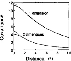
Figure 1 presents numerical examples of the equilibrium covariance functions for the special cases of (radially) symmetric Gaussian and exponential dispersal functions (derived in APPENDIX 11). This confirms that, for distances larger than the neighborhood radius ( r

>

2& 1 or 21 in one or two dimensions), the equilibrium covariance decreases with distance in a way that is nearly independent of the form of the dispersal function. In other words, the form of the dispersal function has an appreciable influence on the equilibrium covariance function only over short distances, within a neighborhood. Figure 1 also shows that under weak selection the covariances within a neighborhood are roughly constant, confirming the internal consistency of the model.

(5)

Isolation by Distance 447

Distance, r l l

FIGURE 1 .-Equilibrium covariance between expected pheno-

types of individuals as. distance between them in one- and two- dimensional habitats. Dispersal is assumed to follow a (radially) symmetric Gaussian or exponential function (solid or dashed lines respectively). Covariances are scaled in units of VplN, the expected additive genetic variance within local populations divided by the neighborhood size. The Euclidean distance, r , is expressed in units of 1, the standard deviation of the dispersal distance per generation along a single spatial axis. The intensity of stabilizing selection on the phenotype is s = 0.0 1.

=.

10-2

0 10-3

10"

'"b

20 4 0 6 0 8 0 100

s = 0.01

0

10'

1 i

10'2 s = 0.01

10''

0 20 4 0 6 0 8 0 100

Distance, rll Distance, rll

FIGURE 2.-Equilibrium covariance between expected pheno-

types of individualsvs. distance in one- and two-dimensional habitats with Gaussian dispersal functions for different strengths of stabilizing selection, s. Covariances are plotted logarithmically in units of

V J N .

strength of selection on the equilibrium pattern of geographic variation is presented in Figure

2

for a Gaussian dispersal function. Figure

2

confirms that the equilibrium geographic variance is much smaller in a two-dimensional habitat than in a one-dimensional habitat and that the geographic covariance decreases more rapidly with distance in two dimensions than in one dimension. It also illustrates the relatively weak dependence of the geographic variance on the strength of selection in a two-dimensional habitat.

Neighborhood sizes under which random genetic drift can cause substantial geographic variance are evaluated numerically in Table 1. These indicate that, especially in two dimensions, a combination of small neighborhood size and extremely weak selection are required to produce substantial geographic variance.

MAINTENANCE OF GENETIC VARIANCE

The expected genetic variance within local populations, V,, is determined by a balance between the losses from selection and random genetic drift, and inputs from mutation and immigration. Assuming that selection is weak and that all of the genetic variance is

TABLE 1

Maximum neighborhood sizes, N, for the equilibrium

geographic variance among local populations to exceed the

phenotypic variance within localities ( ~ ( 0 ) > u t ) in habitats of

different dimensionality

Dimensions Heritability" f i , / c Maximum N

0 Arbitrary 10 50

100 5,000

1,000 500,000

1 0.5 10 8.8

100 88.6

1,000 886

2 0.5 10 2.3

100 4.6

1,000 6.9

a The heritability of the character is h2 = Vg/u2, where V, is the

expected additive genetic variance and u2 is the total phenotypic variance within localities. f i J u measures the width of the adaptive zone for the expected local phenotype in units of u. A habitat of zero dimensions refers to an isolated panmictic population of effective size N . From text Equations 12a and 13a and LANDE (1 976).

additive, using CROW and KIMURA'S (1 964) model of mutation in a quantitative character with multiallelic loci, V, obeys the approximate dynamics (KEIGHTLEY and HILL 1988; BURGER, WAGNER and STETTINGER

1989; LYNCH 1988a)

AVg(t) = - 8 ( t ) s ( t )

-

V & ) / ( 2 N )

+

v,

+

'/zV;(t). (14)

The first term on the right is the loss from selection, where s ( t ) = V,(t)/VS. In TURELLI'S (1984) house-of- cards approximation, P ( t ) = a2/2 is a constant where a is the change in average effect produced by a new mutation, assumed to be the same for all alleles at all loci. In KIMURA (1 965) and LANDE'S (1975) Gaussian allelic approximation, P ( t ) V & t ) / ( 2 n E ) where nE is the effective number of segregating loci. For large populations, the house-of-cards approximation is most accurate if the allelic mutation rate is much less than the strength of selection, p

<<

a 2 / ( 2 V s ) , whereas the Gaussian allelic approximation is most accurate under the opposite condition (TURELLI 1984; SLATKIN

1987). N is the neighborhood size, and V,,, is the additive genetic variance produced by mutation per generation.

The last term in Equation 14 involves V ; ( t ) , the variance in the expected phenotype among localities from which an individual at a given location is likely to have originated. The contribution from recombi- nation of linkage disequilibrium within localities has been neglected for the following reasons. In the absence of selection, linkage disequilibrium within local populations caused by random genetic drift and immigration is as often positive as negative and is zero

(6)

R. Lande

leles at different loci within populations, but if selection is weak and linkage is not very tight the resulting linkage disequilibrium is negligible (LANDE 1975; TURELLI 1984).

I now show that under weak selection the input of genetic variance from immigration at equilibrium,

l/zV;(~), nearly cancels the loss from random genetic drift, -VA=)/(SN). The contribution from migration can be evaluated from the definition

The last term is the convolution of cxx) with m2*(x), evaluated at x = 0. For brevity I analyze only the equilibrium pattern of geographic variation under Gaussian dispersal, writing V, and V; for the equilibrium values. From Equation

7

m

vi

=

( v g / ~ )

(1

-

s)2j-2[m2j*(0)

-

m2Ci+l)* (0)l. (16)

The Gaussian dispersal function and its convolutions are given in APPENDIX 11. In a one-dimensional habitat, from (AB)

j- 1

V; = (Vg/N) (1

-

~ ) ' j - ~ [ j-'/*

-

( j

+

I)-'/~]

m

j- 1

= (V,/N)( 1

-

S)+

m

-

(1 +[1-(1-s)4] (1

-

s)zjj"'2}. (1 7) j = 1

Under weak selection the summation in (17) can be approximated by an integral,

in which the integration from j

-

'/n

to j

+

'/2 corre-

sponds to the j t h term in the summation. This can be evaluated by substituting u =

4,

giving

Vi (Vg/N)[ 1

-

&!-

xs+2(1

+ ~ ) S I

for s<< 1, (18)

and

'/2 (V;

-

Vg/N) -(V,/N) (19)

For Gaussian dispersal in a two-dimensional habitat, using (16) and (AS) with GRADSHTEYN and RHYZIK

(1965, No. 1.513.5),

m

V; = (Vg/N)

2

(1

-

s)'j-?-'(j

+

j - 1

= (V,/N)( 1

-

s)-'[ 1

+

(2s

-

s2) (1

-

~)-~1n(2s

-

s2)]

s (V,/N){l

+

2s[ln(2s)

+

11)

for s

<<

1. (20) Hence

'12 (Vi

-

V,/N) (V,/N)s[ln(Ps)

+

13. (21)

It can be seen from (19) and (21) that under weak selection the rate of loss of genetic variance within neighborhoods from the combination of random

ge-

netic drift and immigration is much smaller than -Vg/(2N). The minimum neighborhood size for the genetic variance maintained within local populations to be at least half that in an infinite panmictic population can be derived from (21) by requiring

'/2 (V,/N

-

Vi) 5 sps (22) where 6 = 1 in the house-of-cards approximation, and 6 = 3 in the Gaussian allelic approximation.

For example, consider a population with Gaussian dispersal in a one-dimensional habitat. Using (19) in the house-of-cards approximation the preceding condition becomes

N L

&i&

(V,/a'). (234

When (22) is an equality, (14) implies V, = V,,,Vs/a2, and because V, increases monotonically with N, (23a) is satisfied if

N 2 (27rVm)1/2Vs/a9. (23b)

Choosing a scale of measurement on which the environmental variance is unity, V, = 1, and defining n as the number of mutable loci influencing the character, parameter values for a typical character are thought to be roughly V, = 25, V, = 0.001 and n p = 0.01 (LANDE 19'75, 1980; TURELLI 1984; ENDLER 1986; LYNCH 1988b). The last two of these imply a2 = 0.05 since with exchangeable loci, V, = 2npa2. With these parameters, (23b) becomes N 2 177, and with larger neighborhood sizes V, approaches 1 .O and the heritability approaches 0.5.

Using (19) in the Gaussian allelic approximation, condition (22) becomes

N L (72E/3)&&. (244

When (22) is an equality (14) implies V, =

( nEVmVs/2)'/', and because V, increases monotonically with N , (24a) is satisfied if

(7)

Isolation by Distance 449

With the above parameters for a typical quantitative character, and n~ = 10 (LANDE 1980, 1981), (24b) becomes N 2 70, and with larger neighborhood sizes V, approaches 0.71 and the heritability approaches 0.41.

With Gaussian dispersal in a two-dimensional habitat, similar conditions can be derived for the expected genetic variance within a locality to be at least half that in an infinite panmictic population. Using (2 1) in the house-of-cards approximation, condition (22) becomes

N 2 -[ln(2s)

+

1]2Vg/a2 (254

or

N 2 -[ln(2Vm/a2)

+

1]2VmV,/a4. (25b)

With the genetic parameters as before, this gives

N 44.

Using (21) in the Gaussian allelic approximation, condition (22) becomes

N 2 -[ln(2s)

+

1]2n~/3 (264

or

N 2 -{% In(2nEVm/Vs)

+

1)2nE/3. (26b) With the same parameters as above, this gives N 2 17. Thus, with these typical parameter values, populations in a two-dimensional habitat with neighborhood sizes larger than a few dozen individuals can maintain most of the additive genetic variance that would occur in an infinite panmictic population, In a one-dimensional habitat, neighborhood sizes several times larger would be required to maintain comparable levels of heritable variation.

DISCUSSION

For a population with a continuous spatial distribution, random genetic drift involves spatially autocorrelated sampling variation in the expected phenotypes at different localities. The present models assume that stabilizing natural selection acts toward the same optimum phenotype in every location, and that the distribution of environmental effects is spatially homogeneous. All geographic variation is therefore caused by random genetic drift.

The pattern of geographic variation in any generation, t , is described by the covariance between expected phenotypes of individuals as a function of the displacement, x, between them in a one- or two- dimensional habitat, c,(x). Apart from sampling er- rors, this is equivalent to the covariance between actual individual phenotypes as a function of distance. With a uniform population density and spatially homogeneous dispersal and selection, c , ( ~ ) is a function

of the Euclidean distance, r , between expected phenotypes.

The equilibrium pattern of geographic variation is approached on a time scale of 1/(2s) generations, where s = Vg/Vs in which V, is the expected additive genetic variance within localities, and l/Vs is a meas- ure of the strength of stabilizing selection

(e

indicates the width of the adaptive zone for the expected phenotype) (LANDE 1976). The geographic variance is proportional to V J N , the approximate sampling variance in the expected local phenotype per generation, where N is the general neighborhood size defined with respect to WRIGHT'S (1969) formulas for Gaussian dispersal. Because actual dispersal functions usually are leptokurtic [WRIGHT (1969, Ch. 12; 1978, Ch. 2); SHIELDS (1982, Ch.

2);

CHEPKO-SADE et al. (1 987)], an arbitrary (radially) symmetric dispersal function was analyzed. Dispersal distances were scaled to have variance 1' of offspring-parent displacement along a single spatial axis, around a mean displacement of 0.

The dimensionality of the habitat has a major influence on the balance between random genetic drift and stabilizing selection. T o simplify the comparison of habitats of different dimensionality, the equilibrium geographic variance can be expressed in multiples of Vg/N. For an isolated panmictic population (in a habitat of zero dimensions) with an effective size N the equilibrium variance in the mean phenotype is then 1/(2s) (LANDE 1976), and, under weak selection, the equilibrium geographic variance in a one-dimensional habitat is approximately and that in a two- dimensional habitat is roughly -ln(2s). Analogous results have been obtained for the equilibrium heterozygosity, but with the formulas inverted and the mutation rate in place of s (MAL~COT 1948, 1969; KIMURA and CROW 1964; NACYLAKI 1989). The ex- istence of substantial geographic variance requires a combination of small neighborhood size and extremely weak selection, especially in two dimensions, as shown in Table 1. Because neighborhood sizes that have been measured in a variety of species are usually larger than a few dozen individuals [WRIGHT (1978, Ch. 2); BARROWCLOUGH (1980); CHEPKO-SADE et al.

(1987)], localized dispersal greatly reduces geographic variance due to random genetic drift in continuously distributed populations.

The equilibrium covariance between expected phenotypes of individuals as a function of the distance between them decreases on a length scale of 1/&,

(8)

distance in a one-dimensional habitat, in proportion to and in two dimensions the decline is faster than exponential proportional to K , , ( f i ( r / l ) ) or

roughly

a

e-A(r/’). Similar results for a single locus were derived by M A L ~ C O T (1 969) for the probability of allelic identity by descent, and by KIMURA and WEISS (1 964) for the correlation of allele frequencies, but with the rate of mutation or long-distance dispersal in place of s. Based on the work of MAL~COT

(1 975), the present findings for phenotypic evolution in infinite one- and two-dimensional habitats should also apply approximate1 to finite habitats if their size is much larger than 1/

f

2s.

Although the equilibrium geographic variance may be small, even under rather weak selection, dispersal of geographic variance created by random genetic drift nevertheless constitutes an important mechanism maintaining genetic variance within local populations. The genetic variance lost within local populations by random genetic drift is converted to geographic variance among localities, and this is recycled via dispersal back to genetic variance within local populations. For a population in a two-dimensional habitat with neighborhood size larger than a few dozen individuals, under an intensity of stabilizing selection representa- tive of univariate selection studies, typical rates of production of additive genetic variance by mutation can maintain most of the heritable variance within neighborhoods that would occur in an infinite panmictic population. In a one-dimensional habitat, neighborhood sizes would have to be several times larger to maintain comparable amounts of heritable variation.

1 thank THOMAS NACYLAKI for extensive helpful discussions, and N. BARTON, T . NACYLAKI, M. SLATKIN and an anonymous reviewer for criticism of the manuscript. This work was supported by U. S. Public Health Service grant GM27 120.

LITERATURE CITED

ABRAMOWITZ, M . , and I. A. STEGUN, 1972 Handbook of Mathe- matical Functions. Dover, New York.

BARROWCLOUGH, G. F., 1980 Gene flow, effective population sizes, and genetic variance components in birds. Evolution 34:

BULMER, M. G., 1985 The Mathematical Theory of Quantitative Genetics, Ed. 2. Oxford University Press, New York.

BURGER, R., G. P. WAGNER and F. STETTINGER, 1989 How much heritable variation can be maintained in finite populations by mutation-selection balance? Evolution 43: 1748-1766. CHEPKO-SADE, B. D., W. M. SHIELDS, J. BURGER, Z. T . HALPIN, W.

T. JONES, L. L. ROGERS, R. P. ROOD and A. T. SMITH, 1987 The effects of dispersal and social structure on effective population size, pp. 287-321 in Mammalian Dispersal Patterns,

edited by B. D. CHEPKO-SADE and Z. T. HALPIN. University of Chicago Press, Chicago.

CROW, J. F., and M . KIMURA, 1964 The theory of genetic loads, Proc. XI Int. Congr. Genet. 3: 495-505.

CROW, J. F., and M. KIMURA, 1970 An Introduction to Population Genetics Theory. Harper & Row, New York.

789-798.

ENDLER, J. A., 1986 Natural Selection in the Wild. Princeton Uni- versity Press, Princeton, N.J.

FALCONER, D. S., 1968 Introduction to Quantitative Genetics, Ed. 2. Longman, London.

FEUENSTEIN, J., 1975 A pain in the torus: some difficulties with models of isolation by distance. Am. Nat. 109: 359-368. ~RADSHTEYN, I. S., and I . W. RYZHIK, 1965 Tables of Integrals,

Series, and Products. Academic Press, New York.

KEIGHTLEY, P. D., and W. G. HILL, 1988 Quantitative genetic variability maintained by mutation-stabilizing selection balance in finite populations. Genet. Res. 52: 33-43.

KIMURA, M., 1965 A stochastic model concerning the maintenance of genetic variability in quantitative characters. Proc. Natl. Acad. Sci. USA 5 4 731-736.

KIMURA, M., and J. F. CROW, 1964 The number of alleles that can be maintained in a finite population. Genetics 4 9 725- 738.

KIMURA, M., and G. H. WEISS, 1964 The stepping stone model of population structure and decrease of genetic correlation with distance. Genetics 4 9 561-576.

KINGMAN, J. F. C., 1977 Remarks on the spatial distribution of a reproducing population. J. Appl. Probab. 1 4 577-583. KORN, G. A., and T . M. KORN, 1968 Mathematical Handbook for

Scientists and Engineers, Ed. 2. McGraw-Hill, New York. LANDE, R., 1975 The maintenance of genetic variability by mu-

tation in a quantitative character with linked loci. Genet. Res.

LANDE, R., 1976 Natural selection and random genetic drift in phenotypic evolution. Evolution 3 0 314-334.

LANDE, R., 1980 Genetic variation and phenotypic evolution dur- ing allopatric speciation. Am, Nat. 1 1 6 463-479.

LANDE, R., 1981 The minimum number of genes contributing to quantitative variation between and within populations. Ge- netics 9 9 541-553.

LYNCH, M., 1988a The divergence of neutral quantitative characters among partially isolated populations. Evolution 42: 455- 466.

LYNCH, M., 1988b The rate of polygenic mutation. Genet. Res.

MALECOT, G., 1948 Les Mathimatigues de I’Hiriditi. Masson et

MALECOT, G., 1967 Identical loci and relationship. Proc. Fifth

MALECOT, G., 1969 The Mathematics of Heredity. W. H . Freeman,

MAL~COT, G., 1975 Heterozygosity and relationship in regularly subdivided populations. Theor. Popul. Biol. 8: 2 12-24 1 . NAGYLAKI, T . , 1974 The decay of genetic variability in geograph-

ically structured populations. Proc. Natl. Acad. Sci. USA 71:

NAGYLAKI, T., 1989 Gustave Malkot and the transition from classical to modern population genetics. Genetics 122: 253- 268.

OBERHETTINGER, F., 1990 Tables ofFourier Transforms and Four- ier Transforms of Distributions. Springer-Verlag, New York. ROUHANI, S., and N. BARTON, 1987 Speciation and the “shifting

balance” in a continuous population. Theor. Popul. Biol. 31:

SAWYER, S., 1977 Asymptotic properties of the equilibrium probability of identity in a geographically structured population. Adv. Appl. Probab. 9 268-282.

SHIELDS, W. M., 1982 Philopatry, Inbreeding, and the Evolution of

Sex. State University of New York Press, Albany.

SLATKIN, M., 1978 Spatial patterns in the distributions of polygenic characters. J. Theor. Biol. 70: 213-228.

SLATKIN, M . , 1987 Heritable variation and heterozygosity under a balance between mutations and stabilizing selection. Genet. Res. 50: 53-62.

2 6 221-235.

51: 137-148.

Cie, Paris.

Berkeley Symp. Math. Stat. Probab. 4: 317-332. San Francisco.

2932-2936.

(9)

Isolation by Distance 45 1

SUDBURY, A., 1977 Clumping effects in models of isolation by distance. J. Appl. Probab. 1 4 391-395.

TAYLOR, R. A. J., 1978 The relationship between density and

distance of dispersing insects. Ecol. Entomol. 3: 63-70. T A Y L O R , R. A. J., 1980 A family of regression equations describ-

ing the density distribution of dispersing organisms. Nature

TURELLI, M., 1984 Heritable genetic variation via mutation-selec- tion balance: Lerch's zeta meets the abdominal bristle. Theor. Popul. Biol. 2 5 138-193.

2 8 6 53-56.

WRIGHT, S., 1943 Isolation by distance. Genetics 28: 114-138. WRIGHT, S., 1946 Isolation by distance under diverse systems of

mating. Genetics 31: 39-59.

WRIGHT, S,, 1951 The genetical structure of populations. Ann. Eugen. 15: 323-354.

WRIGHT, S., 1968 Evolution and the Genetics of Populations, Val. 1. Genetic and Biometric Foundations. University of Chicago Press, Chicago.

WRIGHT, S., 1969 Evolution and the Genetics of Populations, Val. 2. The Theory of Gene Frequencies. University of Chicago Press, Chicago.

WRIGHT, S., 1978 Evolution and the Genetics ofPopuhtions, Val. 4.

Variability within and among Natural Populations. University of Chicago Press, Chicago.

Conmunicaring editor: B. S. WEIR

APPENDIX I

Substituting the first two terms of (lob) into (9), the denominator of the integral can be factored as (I/z 12ET[

+

s)(% 1

+

2

-

s). Decomposing the integral into partial fractions produces

in which A = Vg/[12D(1

-

s)], u 2 = 2s/12 and b 2 =

In a one-dimensional habitat (d = 1), this gives 2(2

-

S ) / F

(OBERHETTINGER 1990, p. 11 No. 3.1)

c,(x) g '/2 A(a-'e-"'

-

b-le-br) (A2)

(which is exact for a symmetric exponential dispersal function). When s

<<

1, this produces text Equations

12a and 12b.

In a two-dimensional habitat ( d = 2), the radial symmetry of the dispersal function and cm(x) can be used to simplify the integrals in (Al). First, expand the exponentials into sine and cosine terms and note that the integrals containing sine (an odd function) vanish, producing two integrals of the form

m m

in which y = a or b. Next, set x 2 = 0, x1 = (-43)

r , and

transform to polar coordinates, 6 1 = Y cos @ and [2 = v sin 6, giving

7- m

I

-

A

7

cos(rv cos @)v

dud@ (A4)

4 2 v 2

+

y2

0 0

Then using ABRAMOWITZ and STEGUN (1972, No. 9.1.1 8), followed by GRADSHTEYN and RHYZIK (1965, p. 678, No. 6.532.4), yields

m

Z

=

A

s

*

du =

-

A K o ( y r ) (A5) 27r Y 2

+

y2 2a

0

where

lo(

e ) and K O ( . ) are, respectively, the Bessel

function and the modified Bessel function of the second kind of order zero. Thus in two dimensions (Al) becomes

c,(x) ( A / P r ) [ K o ( a r )

-

Ko(br)J ( 4

which produces text Equation 13b. Equations 13a and 13c follow from the relations (ABRAMOWITZ and STE-

GUN 1972, pp. 375 and 378)

K&)

=

-In(?) for y + 0

~ ~ ( y )

=

e-y for y

>

1.

APPENDIX I1

Gaussian dispersal: In a habitat of dimensionality

d , with l 2 as the mean squared dispersal distance along one axis, the Gaussian dispersal function is

m ( x ) = (27r12)-d/2 exp{-r2/212) (A7)

and using Fourier transforms it is readily shown that

&*(X) = (47~jZ~)"j/~ exp{-r2/4jl2}. (AS)

From text Equation

7

the dynamics of the covariance between the expected phenotypes of individuals separated by a distance r , starting from a spatially uniform population, are

I

c t ( x ) = (v,/N)

2

(1

-

s)'~-'~-"/'exp{-r'//4j121.

j = 1

(A9)

In a two-dimensional habitat (d = 2) the geographic variance approaches the equilibrium value (using GRADSHTEYN and RYZHIK, 1965, No. 1.5 13.4)

c,(o) = - ( v ~ / N ) ( ~

-

s)-*In(2s

-

s')

-(Vg/N)ln(2s) for 2s

<<

1 (A10)

in agreement with text Equation (1 3a).

(10)

defining 1' as in text Equation 1 la, the exponential dispersal function is

m ( x ) =

(4

z)-~

exp{-&(r/Z)] ( ~ 1 1 )

which has the Fourier transform M ( [ ) = (['Z2/2

+

1)" (OBERHETTINGER 1990, p. 1 1 , No. 3.1). Substi-

tuting this into text Equation (9), the denominator of the integral can be factored as [['Z2/2

+

2

-

s][['Z2/2

+

s], giving (OBERHETTINGER 1990,

p.

5, No. 1.34)

Cm(X) = &(Vg/N)(l

-

s)-'(B-le-Br/'

-

A-le-Ar/l)

(A1 2)

where A =

m,

B

=

f i

and N = 2& 1D. T h e equilibrium geographic variance is then

C,(O) =

J;;

(Vg/N)(1

-

s)"(./5-S

-

&)/

(A 13)

E

< v , / N > ~

for

2s

e<

1

in agreement with text Equation 12a.

In a two-dimensional habitat, defining 1' as in text

Equation 1 l b , the exponential dispersal function is

m ( x ) = 3(2nl2)" exp{-&(r/Z)]. (A14)

Because M ( [ ) is radially symmetric, the double integral in (8) can be simplified by setting [Z = 0,

El

= u and

transforming to polar coordinates, x1 = r cos 6 and xz

= r sin 8. Then from ABRAMOWITZ and STEGUN (1 972, No. 9.1.18) and GRADSHTEYN and RYZHIK (1965, No. 6.623.2) with I'(3/2) = &/2, we obtain the Fourier transform

M([)

=

[(e:

+

4:)Z2/3

+

1 ]-"'. Radial sym- metry of [,(x) can be used as above to simplify the double integral in (9), by setting x2 = 0, x1 = r , and transforming to polar coordinates, = u cos

4

and

t2

= v sin

4.

Then from ABRAMOWITZ and STECUN (1972, No. 9.1.18) and substituting u = u l , we have

m

c m ( x ) = 2(Vg/N)

J

[ u / F ( u ) ] J ~ ( u r / l ) d u (A14)

0