Copyright2001 by the Genetics Society of America
Detection of Closely Linked Multiple Quantitative Trait Loci
Using a Genetic Algorithm
Reiichiro Nakamichi, Yasuo Ukai and Hirohisa Kishino
Laboratory of Biometrics, Graduate School of Agricultural and Life Science, University of Tokyo, Tokyo 113-8657, Japan Manuscript received August 17, 2000
Accepted for publication February 5, 2001
ABSTRACT
The existence of a quantitative trait locus (QTL) is usually tested using the likelihood of the quantitative trait on the basis of phenotypic character data plus the recombination fraction between QTL and flanking markers. When doing this, the likelihood is calculated for all possible locations on the linkage map. When multiple QTL are suspected close by, it is impractical to calculate the likelihood for all possible combinations of numbers and locations of QTL. Here, we propose a genetic algorithm (GA) for the heuristic solution of this problem. GA can globally search the optimum by improving the “genotype” with alterations called “recombination” and “mutation.” The “genotype” of our GA is the number and location of QTL. The “fitness” is a function based on the likelihood plus Akaike’s information criterion (AIC), which helps avoid false-positive QTL. A simulation study comparing the new method with existing QTL mapping packages shows the advantage of the new GA. The GA reliably distinguishes multiple QTL located in a single marker interval.
M
ANY traits of plants and animals are quantitative; sion method that can decrease the computation. This that is, the phenotype of the trait is continuous regression method examines the existence of a QTL and described by measurement values. In many cases, using the information of flanking markers and pheno-one quantitative trait is controlled by multiple genetic typic value, but estimates parameters using multiple re-loci with relatively small effects each. Furthermore, as gression rather than explicit ML. The regression quantitative traits fluctuate under the influence of envi- method reduces the calculation task, but the approxima-ronmental effects, we cannot infer a genotype from tion is not so good (Kao 2000).a phenotype unambiguously. Therefore, genetic and The SIM method is biased, when there are multiple environmental effects contributing to the target traits QTL, because it assumes only one QTL at a time. To must be estimated using information from phenotypic correct for this bias, Zeng (1993, 1994) and Jansen values and molecular markers to locate quantitative trait (1993) independently developed composite interval loci (QTL) on linkage maps. mapping (CIM). CIM is a combination of SIM and multi-The simple interval mapping (SIM) approach of ple regression. When testing a QTL using the method LanderandBotstein (1989) examines the existence of interval mapping, CIM uses the genotypes of the of a QTL at each location on the linkage map. The markers (except for the flanking markers of the target likelihood is calculated from (a) the conditional proba- QTL) as covariates to control genetic effects at other bility of the QTL genotype given the marker genotype than the target QTL. However, if there are multiple and (b) the conditional distribution of the phenotypic QTL within a marker interval, neither CIM nor SIM can value given the QTL genotype. The existence of the QTL detect them separately.
is evaluated by the log-likelihood ratio (called the LOD It is possible to construct a genetic model that consid-score), comparing the proposed QTL with the “no QTL” ers multiple QTL simultaneously. Because we do not hypothesis. The LOD score is calculated at all the loca- know the number of QTL in advance, it is impractical tions on the linkage map, and, if a peak of the LOD to calculate the LOD scores for all possible combina-score is higher than a given threshold, a QTL is mapped tions of number and locations of QTL. We require a at the point. SIM uses the expectation maximization practical method to simultaneously estimate the opti-(EM) algorithm to estimate the maximum-likelihood mum number of QTL. Because the LOD score drops at (ML) point, and the calculation is fairly computationally the positions of markers and consequently shows many expensive.HaleyandKnott(1992) described a regres- local optima, most numerical optimization procedures
using information based on the local shape of the LOD score, such as the Newton-Raphson procedure and the
Corresponding author:Reiichiro Nakamichi, Laboratory of Biomet- simplex method, do not perform so well.
rics, Graduate School of Agricultural and Life Science, University of
Bayesian analysis of QTL using Markov chain Monte Tokyo, Yayoi 1-1-1, Bunkyo, Tokyo 113-8657, Japan.
E-mail: [email protected] Carlo (MCMC) has been reported recently (Uimariand
Hoeschele1997;StephensandFisch1998;Sillanpa¨a¨ andArjas1998;YiandXu2000). This method searches
for the best combination of the QTL number and loca- Figure1.—GA genotype.M, number of QTL;C
j, chromo-tions by using a prior distribution to update the parame- some on whichjth QTL exists;Lj, location of thejth QTL on
the chromosomeCj(j⫽1, 2, . . .,M). ters of the model step by step, which enables us to
evaluate the reliability of the estimates in terms of a posterior distribution. However, the approach is
pres-whereis a constant value that has no relation to the ently computationally prohibitive, and thus it is often
QTL genotype, andeis the residual following a normal difficult to detect QTL correctly in a realistic time
pe-distribution with mean zero and constant variance. The riod.
termgm(m⫽ 1, 2, . . .M) is the genetic effect of the KaoandZeng(1997) andKaoet al.(1999) described
mth QTL. Let the allele from P1be denoted byQmand a general model for handling multiple QTL
simultane-the allele from P2 be denoted by qm; thengmtakes am, ously. This model includes not only additive effects of
dm, and⫺amfor the QTL genotypesQmQm,Qmqm, andqmqm, QTL but also epistatic effects between QTL. Their
pro-respectively. The additive effect,am, and the dominance posed multiple interval mapping (MIM) searches for
effect,dm, may be either positive or negative. For simplic-the best model with a stepwise selection using
likeli-ity, we assume there are no epistatic effects. hood-ratio statistics to add or to delete a QTL.
Thresh-Given a set of the locations of QTL, we can evaluate old values for QTL detection were calculated assuming
the plausibility of the set using likelihood. Therefore, a2distribution of the ratio statistics plus a Bonferroni
QTL mapping is a case of combinatorial optimization, correction for multiple testing of marker intervals
which must search for the combination of locations on (LanderandBotstein1989;Zenget al.1999).
a linkage map, which maximizes the likelihood. As an alternative with high potential, we propose and
The GA is a numerical optimization procedure, based test a genetic algorithm (GA) for QTL mapping. We
on an analogy to organic evolution. Candidates for the use a multiple-QTL model and Akaike’s information
optimum solution are coded as the “genotypes” of vir-criterion (AIC,Akaike1974) as the evaluation function.
tual creatures (GA individuals), and candidates have a Because AIC measures predictive power for the
distribu-probability of survival described by the “fitness.” First, tion of quantitative traits, it is particularly useful for the
a population of GA individuals with random genotypes application to breeding such as marker-assisted
selec-is generated. Then, “mating” among the GA individuals, tion. Candidates for the QTL numbers and locations
“mutation,” and “selection” by the fitness are repeated are encoded as “genotypes” of the GA. “Selection” on
to improve fitness until the fitness in many succeeding the genotype then produces an efficient global search
generations changes by less than a threshold value. At after maintaining diversity in the GA population
this time, the genotype of the best GA individual is through “crossover” and “mutation” type operations. A
adopted as the optimum solution. “Mating” and “muta-combination of “drastic mutation” and “slight
modifica-tion” increase the diversity of the GA population, while tion” enables efficient global search for QTL number
“selection” reduces it. For GA to reliably find a good and locations.
global optimum, the factors in quotation marks need A major advantage of using AIC for QTL mapping
to be appropriately matched to the problem. comes when the prime interest is marker-assisted
breed-GA genotype:In our GA, the genotype is the number ing. Here a major problem is not detecting closely
and location of QTL. Figure 1 shows the GA genotype. linked QTL of opposite effect (a type II error), and so
Mdenotes the number of QTL. The term (Cx,Lx) denotes not checking the results of offspring where
re-the location of re-thexth QTL, whereCxis the chromosome arrangement has occurred. In general, it is very difficult
on which the xth QTL exists, and Lx is the location to control type II error rates. Most of the proposed QTL
measured in centimorgans on the chromosomeCx. mapping methods control type I error rates with no
Selection function and alternating generations: The regard to type II error rates. However, by maximizing
tournament method is adopted as the “selection” of predictive power, AIC creates a balance of type I and
parent GA individuals that breed offspring GA individu-type II errors, and in this sense is desirable in
marker-als. Figure 2 gives an example where some constant assisted breeding QTL prediction.
numberNt(called the tournament size) of the GA
indi-viduals is extracted (tournament 1) from the GA popula-MODEL AND GENETIC ALGORITHM tion of the current generation. Next, the GA individual with the highest fitness (here, the lowest AIC) among Let us consider an F2population from two completely
tournament 1 is adopted as a parent GA individual (par-homozygous parents P1 and P2. Let the number of the
ent 1). This parent selection is repeated again without QTL beM.The phenotypic valueYof one F2individual
replacement (so we get parent 2 from tournament 2), is expressed as
and the genotype of the offspring GA individual is cre-ated from the genotypes of the selected two parents
Figure 2.—Overview of GA.NGA, number of GA
indi-viduals;Nt, tournament size;
Pd, probability of drastic
mu-tations;Ni, number of
iden-tical GA individuals with newly created GA individual in the next generation; Ps,
base probability of slight mu-tation (slight mumu-tation oc-curs with probability Ps ⫻
Ni); Dshift, distance of slight
shift.
through the “crossover” and mutation. The breeding becomes the same as that of the current generation (dotted line in Figure 2). This alternation of GA genera-procedures are repeated without replacement until the
Figure3.—An example of GA crossover. Parent 1 has two QTL located at (Ca,La) and (Ca,Lb). Parent 2 has four QTL located at (Ca, La), (Ca,Lc), (Cb, Ld), and (Cb,Lf). The QTL
number of the offspring GA individual is selected randomly Figure4.—An example of three patterns of GA mutation. from the range defined by the QTL numbers of parents (here, The offspring created in Figure 3 has adopted the mutation. two to four). The QTL locations of the offspring are selected Insertion adds one QTL on a random location. Deletion se-randomly from these locations. In this example, three loca- lects a QTL randomly and deletes it. Substitution selects a tions, (Ca,Lb), (Ca,Lc), and (Cb,Lf), are selected. QTL randomly and changes to a random location.
fitness appears in successive generations, indicating con- of the GA generation, a GA individual with higher fitness vergence (bold solid line in Figure 2). breeds more offspring than the GA individuals with
GA crossover:GA crossover creates an offspring GA lower fitness. This procedure decreases genotypic diver-individual as shown in Figure 3. There are two parent GA sity of the GA population. If the GA selection drives individuals selected through the tournament method. diversity too low, the GA easily falls into local optima. Parent 1 has two QTL located at (Ca,La) and (Ca,Lb). In our GA system, diversity means the number of the Parent 2 has four QTL located at (Ca,La), (Ca,Lc), (Cb, candidates of the QTL location contained in the GA
Ld), and (Cb,Lf). The number of QTL for the offspring population. Since the GA mutations mentioned above is selected randomly from the range determined by the change GA genotypes drastically, most of them may numbers of QTL of the parents. The upper limit of the be deleted from the population. To help maintain the range is the larger QTL number of the parents, and diversity of the GA population, we introduce very slight the lower limit is the smaller one. In the example in mutation. This additional mutation randomly selects a Figure 3, the upper limit is four (QTL number of parent QTL from a GA individual and moves it a little from its 2), and the lower limit is two (QTL number of parent 1). present location. When an offspring GA individual is Then, the offspring’s QTL number is selected randomly created through crossover and drastic mutation, if GA from two, three, or four, and three is selected in this individuals of identical genotype already exist in the example. There are six QTL locations among the geno- newly created population, the slight shift mutation oc-types of the parents, but the location (Ca,La) is dupli- curs with the probability proportional to the number cated, so there are five available locations, namely, (Ca, of identical GA individuals.
La), (Ca,Lb), (Ca,Lc), (Cb,Ld), and (Cb,Lf). Three loca- GA-controlling parameters: In our GA, five parame-tions are selected randomly from these five locaparame-tions. In ters control the performance: size of GA population, this example, (Ca,Lb), (Ca,Lc), and (Cb,Lf) are selected. tournament size, probabilities of drastic and slight
muta-GA mutation of drastic change: The offspring that tions, and shift distance for the slight mutation. GA the GA individual created through the crossover may population size affects the speed of the search and the be changed further by a random mutation event. GA diversity. Small population size takes less time than a mutation has three patterns (Figure 4), which mimic large one, but a large population contains more candi-real genomic evolution: insertion, deletion, and substi- dates of QTL locations in the GA population, that is, it tution (relocation). When a mutation occurs, one of allows high diversity, while in a small population, diver-these is randomly selected and applied to the offspring sity can quickly decrease. Tournament size affects the GA individual. Insertion adds a random location to the selection pressure. Large tournament size increases the list of QTL locations in the GA genotype, deletion ran- chance to select a GA individual with high fitness at domly selects a QTL from the GA genotype and deletes the expense of diversity. Mutation affects the rate at it, and substitution randomly selects a QTL from the which a promising new QTL location enters into the GA genotype and moves it to a random location on a GA population. A high mutation rate and large shift
random chromosome. distance quickly generate many QTL locations not
have attempted to balance these conflicting require- freedom being the dimension of. Taking the expecta-tion, we get
ments (e.g.,SchraudolpfandBelew1992;Myersand Hancock1997;Streifelet al.1999), there is no general
EX,Y[logeL(ˆ(X)|Y)⫺logeL(ˆ(X)|X)]⫽ ⫺(dimension of).
criterion for setting up these parameters. Accordingly,
GA parameters are typically determined empirically. We By taking account of this difference, AIC is defined as repeated many simulations, changing the GA
control-AIC⫽ ⫺2(maximum log-likelihood) ling parameters, and then selected parameter values
that showed good QTL detection. We settled on the ⫹ 2(the number of parameters). number of GA individuals being 100, the tournament
The model with lowest AIC has maximized predictive size was two, the rate of the drastic GA mutation was
power. The parameters of our model (Equation 1) are 0.05, and the rate of slight mutation was set to be 0.25
the location, additive and dominance effects of each of the number of identical GA individuals to a newly
QTL, the constant value, and the residual variance. So, created GA individual. The slight mutation moves the
forMQTL, selected QTL 1 cM. To maximize the speed and
cer-tainty of convergence to the global optimal point,
fur-GA fitness⫽ ⫺2 max logeL⫹2(3M⫹2). (2)
ther study of GA-controlling parameters is desirable.
Fitness of GA:Fitness is measured by the LOD score, Here, max logeL is the log-likelihood maximized over which expresses the goodness of fit of the model to the the additive and dominance effects of the QTL (am,dm, data. However, the LOD score tends to increase with m⫽ 1, 2, . . . M), the constant (), and the residual the number of QTL, simply because of an additional variance (2), given the locations of the QTL. The
pen-degree of freedom. To avoid the false-positive detection alty of one log-likelihood unit for one additional param-of QTL, we need a penalty on the number param-of QTL. eter is valid under the regularity condition that guaran-Since GA repeats the evaluation of fitness so many times, tees the central limit theorem. When the sample size we need a criterion that is quickly calculated. Further, is not large enough for a good approximation to the in the actual application of QTL analysis to the field of multinormal asymptotic distribution of the parameter breeding such as marker-assisted selection, it is often of estimates, further elaborations become necessary most concern to predict the distribution of quantitative (LanderandBotstein1989;ChurchillandDoerge traits. Accordingly, we adopt AIC as the fitness criterion. 1994;DoergeandChurchill1996;Zenget al.1999). AIC is very simple and was developed to select the model AIC is more liberal than likelihood-ratio hypothesis with the highest expected predictive power (seeAkaike testing procedures, because it may allow the model to 1974; Sakamoto et al. 1983). The fitting of a model incorporate “nonsignificant” QTL, as long as they con-with a parameter vectorto the dataXis expressed as tribute to increasing the predictive power. Like the hy-the maximum log-likelihood pothesis-testing procedure, the procedure based on AIC has some probability of making type I errors. However, max logeL(|X)⫽ logeL(ˆ(X)|X), the predictive power and the accuracy of the estimated
genetic effects are maximized, and, in this sense, an whereˆ is the vector of maximum-likelihood estimates
optimal balance of type I and type II errors is achieved. (MLE) of. Assume that the data setYis independent of
In practical situations, such as marker-assisted selection, Xand follows the same distribution asX.The predictive
it may be advantageous to examine the best AIC model power of the model is measured by logeL(ˆ (X) |Y). On
and exclude QTL with negligible genetic effects. average, this is worse than the maximum log-likelihood
Suppose we have a sample of sizeNfrom the F2
popu-because it is not tailored to the data at hand. The
differ-lation. Each of theMQTL has three possible genotypes, ence in likelihood may be examined with the Taylor
QmQm,Qmqm, andqmqm, indexed askm⫽1, 2, and 3 (m⫽ expansion:
1, 2, . . .M). The genetic effectgm,kmof themth QTL is
am,dm, and⫺amforkm⫽1, 2, and 3. The log-likelihood
EX,Y[logeL(ˆ(X)|Y)]⫽EX,Y[logeL(ˆ(Y)|X)]
function is
ⱌEX[logeL(ˆ(X)|X)]
logeL⫽
兺
N
j⫽1
loge
冦
兺
3k1⫽1
. . .
兺
3
kM⫽1
(Pj,k1,...kMφj,k1,...kM)
冧
, (3)⫹1⁄
2EX,Y[(ˆ(Y)⫺ ˆ(X))⬘
⫻(ⵜⵜ⬘logeL(ˆ(X)|X))
wherePj,k1,...kMis the conditional probability of the QTL’s ⫻(ˆ(Y)⫺ ˆ(X))]. composite genotype given the information of the
mark-ers’ genotypes and Under regularity condition,ˆ(Y)⫺ ˆ (X) asymptotically
follows a normal distribution of mean zero and variance
φj,k1,...kM⫽ 1
√
22 exp冦
⫺(yj⫺ ⫺RMm⫽1gm,km)2
22
冧
. (4)equal to⫺2 · (E[ⵜⵜ⬘logeL(|X)])⫺1.
Hence, Z ⫽ (ˆ(Y) ⫺ ˆ(X))⬘(ⵜⵜ⬘ logeL(ˆ(X) | X)
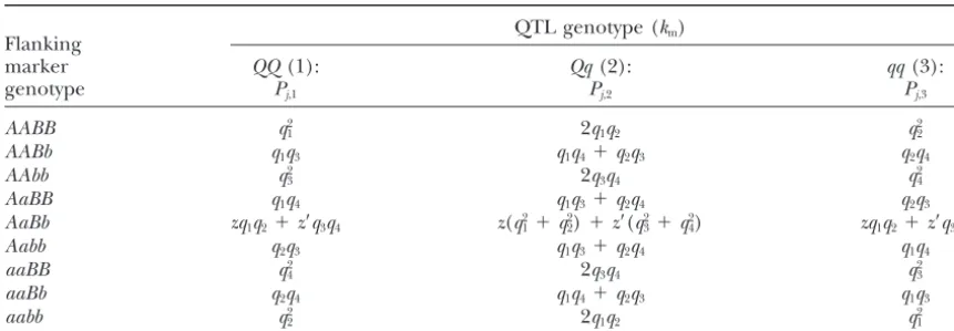
TABLE 1
Conditional probability of the QTL genotype, given flanking marker genotypes
QTL genotype (km)
Flanking
marker QQ(1): Qq(2): qq(3):
genotype Pj,1 Pj,2 Pj,3
AABB q2
1 2q1q2 q22
AABb q1q3 q1q4⫹q2q3 q2q4
AAbb q2
3 2q3q4 q24
AaBB q1q4 q1q3⫹q2q4 q2q3
AaBb zq1q2⫹z⬘q3q4 z(q21⫹q22)⫹z⬘(q23⫹q24) zq1q2⫹z⬘q3q4
Aabb q2q3 q1q3⫹q2q4 q1q4
aaBB q2
4 2q3q4 q23
aaBb q2q4 q1q4⫹q2q3 q1q3
aabb q2
2 2q1q2 q21
A,B, molecular markers;Q, QTL;r1, recombination value betweenAandQ;r2, recombination value between
QandB;r1⫹2, recombination value betweenAandB;r12, probability that recombination occurs at both A–Q
and Q–B intervals;q1⫽(1⫺r1⫺r2⫹r12)/(1⫺r1⫹2);q2⫽r12/(1⫺r1⫹2);q3⫽(r2⫺r12)/r1⫹2;q4⫽(r1⫺r12)/
r1⫹2;z⫽(1⫺r1⫹2)2/{(1⫺r1⫹2)2⫹r1⫹22};z⬘ ⫽1⫺z.
most one QTL,Pj,k1,...kMis the product of the conditional and the M step of maximization of logeL* is repeated
probabilities of the QTL genotypes: until the parameters converge. These crude estimates of genetic parameters are biased because of the effects Pj,k1,...kM⫽
兿
M
m⫽1
P*j,km. (5) of other QTL. Thus, we next apply a moment method
to these crude estimates to remove the effects of other P*j,kmdepends on the genotypes of the two markers flank- QTL. The marginal expectations for these genotypes ing the QTL and on the recombination fraction between are obtained by
them (Table 1;HayashiandUkai1994;KaoandZeng
E[YQmQm]⫽ ⫹
兺
M
h⫽1
{(1⫺2rmh)ah}⫹
兺
Mh⫽1
兵2rmh(1⫺rmh)dh}⫽ ˜m⫹a˜m (7)
1997). Table 1 describes the probabilities for one QTL between two markers. But, there can be multiple QTL
in a marker interval particularly when dense marker E[YQmqm]⫽ ⫹
兺
M
h⫽1
{(1⫺2rmh⫹2r2mh)dh}⫽ ˜m⫹d˜m (8)
linkage maps are not available. In such a case, QTL
other than the target QTL are regarded as markers and E[Y
qmqm]⫽ ⫺
兺
M
h⫽1
{(1⫺2rmh)ah}⫹
兺
Mh⫽1
{2rmh(1⫺rmh)dh}⫽ ˜m⫺a˜m,(9)
used as flanking markers in Table 1. Details of this problem are mentioned in thediscussion.
where rmh is the recombination fraction between the KaoandZeng(1997) andKaoet al.(1999) described
mth andhth QTL. Then, we obtained the final estimates an EM algorithm to estimate the genetic effects of
multi-ˆ and aˆmdˆm(m ⫽ 1, 2, . . . M) by solving the linear ple QTL. With the explicit formula of conditional
proba-equations bilities of genotypes of up to two QTL in a marker
interval, their procedure can detect multiple QTL
suc-a˜m⫽
兺
Mh⫽1
兵
(1⫺ 2rmh)ah其
(10) cessfully. Instead of extending their formula to a generalcase, we adopt the following two-step moment method
for simplicity. First, we obtain the crude estimates of the d˜ m⫽
兺
M
h⫽1
兵
(1⫺ 2rmh)2dh其
(11) genetic effectsa˜m,d˜m, the constant˜m, and the residualvariance˜2
mfor each QTL, assuming a single QTL. These
⫽ ˜m⫺2
兺
M
h⫽1
rmh(1⫺ rmh)dh. (12) estimates are obtained by the EM algorithm. This
re-peats the E step of calculating the expected
log-likeli-hood; hence Likewise, the estimates of the residual variance ˆ2 are
obtained by logeL*⫽
兺
N
j⫽1
兺
3km⫽1
Zj,kmloge(P*j,kmφj,km), (6)
2⫽ ˜2
m⫺2
兺
M h⫽1rmh(1⫺rmh)
兵
a2h⫹(1⫺2rmh⫹2r2mh)d2h其
. (13)where
Since the estimates of and 2 have different values
for eachmin this procedure, we adopt the average as Zj,km⫽
P*j,kmφj,km R3
km⫽1P*j,kmφj,km ˆ andˆ
Figure 5.—Improvement of the fitness of the best GA individ-ual with GA generations.
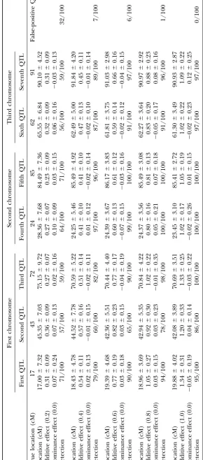
SIMULATION EXPERIMENTS Effects of QTL:Next, we altered the pattern of QTL, so seven QTL were located on three chromosomes at We examined the performance of our GA through a
17, 43, and 72 cM along the first chromosome, 24 and set of numerical experiments using simulated F2
popula-85 cM along the second chromosome, and 62 and 91 cM tions. We used Haldane’s model to generate the marker
along the third chromosome. Each QTL had the same genotype data assuming no interference among
mark-genetic effect. Simultaneously, additive effects were var-ers. The variance of the residual was set at 1.0, and the
ied from 0.2 to 1.0 in steps of 0.2, and the dominance constant value was set at 0. That is, phenotypic value
effects were fixed at 0. data were generated following a normal distribution
The experiments were repeated 100 times. Table 3 with variance 1.0 and mean determined by the
summa-shows the mean and the standard deviation of the esti-tion of the genetic effects of QTL. The sample size of
mates when a QTL was detected at the relevant region. the F2population was set at 500, each F2individual had
It also shows the empirical probabilities of the detection. one or three pairs of chromosomes of 100-cM length
For example, when the additive effect of each QTL was each, and 11 markers were located every 10 cM on each
0.2, the first QTL was detected 71 times out of 100 chromosome.
trials, and the second, 57 times. With increasing genetic In these experiments, the number of GA individuals
effects, it becomes easier to correctly detect QTL. When was 100, and the tournament size was two. The rate of
the additive effects are 1.0, the average probability of the ordinary GA mutation was 0.05, and the rate of the
detection is 0.964, but when the additive effects are additional one was set to be 0.25 of the number of GA
0.2, the average probability is 0.624. False-positive QTL, individuals with the same GA genotype as the one newly
where QTL have negligible genetic effects or are located created. These GA-controlling parameters were exactly
outside the true relevant regions, occurred with an aver-those found to work well empirically.
age frequency of 0.32 with small effects, dropping to
Behavior of the GA: In this experiment, three QTL
0.00 with genetic effects of 1.0. This question of whether were located on the same chromosome at positions of
anything can be done about AIC being too liberal at 17, 43, and 85 cM from the end of a chromosome. Each
lower genetic effects requires further study. The trade-QTL had an additive effect of 1.0 and a dominance
off will likely be decreasing type I errors but more rapidly effect of 0 (broad-sense heritability is 0.6). Figure 5 and
rising type II errors (i.e., failure to include the true Table 2 show that the GA converged by the 20th GA
QTL). generation. The estimates of three QTL had locations
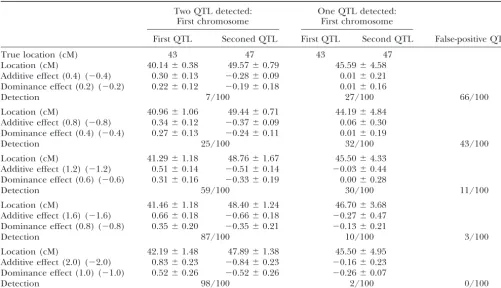
Closely linked QTL:We examined the performance of 16, 84, and 43 cM, and additive effects of 1.424, 1.358,
of our GA in the situations of closely linked QTL (Table and 1.084, all close to the true values. The dominance
4). In this situation, two QTL were located on the same effects were correctly estimated to be negligible. The
chromosome at 43 and 47 cM. As the markers are lo-residual variance was also reliably estimated (0.977vs.
cated every 10 cM, no marker exists between the two 1.0). Repeating the same experiment 100 times (Figure
QTL. These two QTL had reverse genetic effects on 6), we detected three true QTL in 96 out of 100
simula-each other. The additive and dominance effects of the tions, and four QTL, including one false positive, in the
TABLE 2
Improvement of QTL estimation with more GA generations
1st generation 10th generation 20th generation
Location Location Location
(cM) a d (cM) a d (cM) a d
QTL 1 20 ⫺0.441 0.669 15 1.602 ⫺0.022 16 1.424 ⫺0.014
QTL 2 93 1.182 ⫺0.097 87 1.243 ⫺0.036 84 1.358 ⫺0.056
QTL 3 51 1.059 ⫺0.109 50 1.045 ⫺0.100 43 1.084 ⫺0.099
QTL 4 22 1.922 ⫺0.737 — — — — — —
0.147 0.090 0.101
2 1.082 1.100 0.977
Fitness ⫺218.1 ⫺234.2 ⫺242.8
, constant value;2, residual variance;a, additive effect;d, dominance effect.
and 1.0, and those of the QTL at 47 cM were changed Comparison with other methods:We compared the precision of our GA method with those of SIM, CIM, and
from⫺0.4 and⫺0.2 to⫺2.0 and⫺1.0.
The simulations were repeated 100 times. Table 4 Bayesian estimation. Software packages used in these experiments were QTL Cartographer (Basten et al. shows the results. For example, when the additive and
dominance effects of the QTL are 1.6 and 0.8 for the 1998) for simple and composite interval mapping and Multimapper (Sillanpa¨a¨ 1998) for Bayesian estima-QTL at 43 cM and⫺1.6 and⫺0.8 for the QTL at 47 cM,
two QTL with reverse genetic effects were detected 87 tion. For SIM and CIM, the critical value of the LOD score for claiming QTL detection with a 5% probability times out of 100 trials in the marker interval 40–50 cM,
one QTL was detected 10 times, and no QTL was de- of a type I error was based on 1000 replicates of the simulation under the null hypothesis of no QTL. Three tected 3 times. No cases of three QTL being detected
were observed. separate experiments were repeated 100 times, and the
results are summarized in Tables 5 and 6. Here, the estimates of the genetic effects are smaller
than their true values. This bias of the estimated genetic Conditions for generating the data were as above. In the first experiment (Table 5), three QTL were located effects comes from the high correlation between the
two QTL, even conditional on the marker information. on the same chromosome at 17, 43, and 85 cM from the end of a chromosome. Each QTL had an additive However, unlike multicolinearity in regression analysis,
the estimates are conservative rather than liberal, pre- effect of 1.0 and a dominance effect of 0 (broad-sense heritability is 0.6). CIM and GA always detected the venting practitioners from being too optimistic.
TABLE 4
Ability of GA to locate two very close QTL with opposite effects (100 replicates for each combination of additive and dominant effect)
Two QTL detected: One QTL detected: First chromosome First chromosome
First QTL Seconed QTL First QTL Second QTL False-positive QTL
True location (cM) 43 47 43 47
Location (cM) 40.14⫾0.38 49.57⫾0.79 45.59⫾4.58
Additive effect (0.4) (⫺0.4) 0.30⫾0.13 ⫺0.28⫾0.09 0.01⫾0.21 Dominance effect (0.2) (⫺0.2) 0.22⫾0.12 ⫺0.19⫾0.18 0.01⫾0.16
Detection 7/100 27/100 66/100
Location (cM) 40.96⫾1.06 49.44⫾0.71 44.19⫾4.84
Additive effect (0.8) (⫺0.8) 0.34⫾0.12 ⫺0.37⫾0.09 0.06⫾0.30 Dominance effect (0.4) (⫺0.4) 0.27⫾0.13 ⫺0.24⫾0.11 0.01⫾0.19
Detection 25/100 32/100 43/100
Location (cM) 41.29⫾1.18 48.76⫾1.67 45.50⫾4.33
Additive effect (1.2) (⫺1.2) 0.51⫾0.14 ⫺0.51⫾0.14 ⫺0.03⫾0.44 Dominance effect (0.6) (⫺0.6) 0.31⫾0.16 ⫺0.33⫾0.19 0.00⫾0.28
Detection 59/100 30/100 11/100
Location (cM) 41.46⫾1.18 48.40⫾1.24 46.70⫾3.68
Additive effect (1.6) (⫺1.6) 0.66⫾0.18 ⫺0.66⫾0.18 ⫺0.27⫾0.47 Dominance effect (0.8) (⫺0.8) 0.35⫾0.20 ⫺0.35⫾0.21 ⫺0.13⫾0.21
Detection 87/100 10/100 3/100
Location (cM) 42.19⫾1.48 47.89⫾1.38 45.50⫾4.95
Additive effect (2.0) (⫺2.0) 0.83⫾0.23 ⫺0.84⫾0.23 ⫺0.16⫾0.23 Dominance effect (1.0) (⫺1.0) 0.52⫾0.26 ⫺0.52⫾0.26 ⫺0.26⫾0.07
Detection 98/100 2/100 0/100
Estimates of the QTL location and additive and dominance effects are summarized in the form of mean⫾standard deviation on the basis of the replicates in which one or two QTL were detected at the relevant region. Values in parentheses denote the true values of the genetic effects of the QTL at 43 cM (left parentheses) and the QTL at 47 cM (right parentheses). “Detection” denotes the empirical probabilities of the detection of QTL on the basis of 100 replicates. “False-positive QTL” denotes the empirical probabilities of the detection of QTL with negligible little effects or QTL outside of relevant regions.
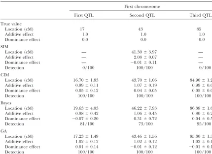
three QTL correctly, but SIM could not detect the three composite interval mapping cannot detect QTL sepa-rately, as in the case of simple interval mapping. Bayes-QTL separately. Bayesian analysis sometimes detected
three QTL, but in other cases it detected only two. The ian analysis can detect QTL separately in such a case, but will not work well if there are many QTL or if the probability of success for the Bayesian analysis was 81/
100 for the QTL at 17 cM, 73/100 for the QTL at 43 cM, amount of information decreases due to QTL having opposite net effects. Moreover, Bayesian analysis is time and 95/100 for the QTL at 85 cM.
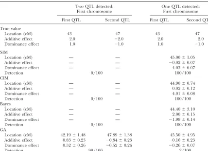
In the second experiment (Table 6), two QTL were intensive, because it uses the MCMC method. We per-formed our experiments on a DEC Alpha 21164A located on the same chromosome at 43 and 47 cM. As
the markers are located every 10 cM, no marker exists 500MHz workstation, and for the three-QTL experi-ment (Table 5), Bayesian analysis took 150–200 min, between the two QTL. The QTL at 43 cM had additive
and dominance effects of 2.0 and 1.0, respectively, while our GA took only 1–3 min.
Since the GA repeats the evaluation of the fitness so whereas the QTL at 47 cM had the opposite effects,
⫺2.0 and⫺1.0 (broad-sense heritability isⵑ0.82). SIM, many times, a criterion that is easily calculated is
re-quired. And as mentioned above, it is often of primary CIM, and the Bayesian method all detected only one
QTL with very little genetic effect because of the two importance to predict the distribution of quantitative traits in the field of breeding such as marker-assisted opposite QTL effects. However, our GA detected the
two QTL in 98 cases out of 100 trials. selection. AIC was developed to select the model with the highest predictive power (Akaike1974;Sakamoto
et al.1983) and is very simple. The GA detects QTL with DISCUSSION
higher probability than the other methods. That is, it shows a significant improvement in type II error rates, Numerical simulations clearly showed the high level
while type I errors are not overly apparent. For the of detection of our GA. Composite interval mapping is
purpose of marker-assisted breeding, this is a major well known as an improved interval mapping. However,
TABLE 5
Comparison of four methods inferring three QTL (100 replicates)
First chromosome
First QTL Second QTL Third QTL
True value
Location (cM) 17 43 85
Additive effect 1.0 1.0 1.0
Dominance effect 0.0 0.0 0.0
SIM
Location (cM) — 41.30⫾3.97 —
Additive effect — 2.08⫾0.07 —
Dominance effect — ⫺0.01⫾0.11 —
Detection 0/100 100/100 0/100
CIM
Location (cM) 16.70⫾1.83 43.70⫾1.06 84.90⫾1.20
Additive effect 0.99⫾0.11 1.07⫾0.19 0.99⫾0.08
Dominance effect 0.05⫾0.12 0.04⫾0.05 0.05⫾0.09
Detection 100/100 100/100 100/100
Bayes
Location (cM) 19.63⫾4.03 46.22⫾7.93 86.38⫾1.69
Additive effect 0.98⫾0.42 1.06⫾0.45 0.80⫾0.21
Dominance effect ⫺0.07⫾0.20 0.31⫾0.72 0.04⫾0.56
Detection 81/100 73/100 95/100
GA
Location (cM) 17.23⫾1.49 43.46⫾1.56 85.30⫾1.53
Additive effect 1.02⫾0.12 1.02⫾0.12 1.02⫾0.12
Dominance effect 0.01⫾0.14 ⫺0.01⫾0.12 ⫺0.01⫾0.16
Detection 100/100 100/100 100/100
Estimates of the QTL location and additive and dominance effects are summarized in the form of mean⫾ standard deviation on the basis of the replicates in which a QTL was detected at the relevant region. “Detection” denotes the empirical probabilities of the detection of QTL on the basis of 100 replicates.
our GA has better performance than all the others, if ble, but we should leave this as an open question for more extensive comparisons.
type I error rate is the sole focus of attention (and in
Dense marker linkage maps presently exist only for fact it should not be, since these methods explicitly
some major plants and animals. Worse, genes control-aim to control type I errors). AIC is a relatively liberal
ling the same trait are often clustered (Meyers et al. criterion, while software packages of interval mapping
1998; Simons et al. 1998). Even though rice is fairly and Bayesian analysis use even more conservative
crite-densely sampled, two important genes in one interval ria. Accordingly, our GA picked up more false-positive
were regarded as a single gene using standard QTL QTL than the other methods. The question of how to
mapping (Wanget al.1999). This suggests that multiple trade off type I (false detections) and type II (failures
QTL may well exist within a given marker interval. If to detect) is an important topic that is yet to be studied.
there are multiple QTL in one marker interval, the In this study, we adopted a moment method to
esti-conditional probabilities of QTL genotypes given mate the genetic effects. On the other hand,Kaoand
marker genotypes are not described by Table 1 and Zeng(1997) andKaoet al.(1999) proposed the MIM
Equation 5. For example, let two QTL (QTL1and QTL2)
using a general EM algorithm for multiple QTL. MIM
exist between two markers (markerAand markerB) in directly implements simultaneous estimation of genetic
the following order: markerA, QTL1, QTL2, and marker
effects. Since the moment method is less statistically
B.The conditional probability of QTL genotypes given efficient than ML, MIM may give more precise MLEs
marker genotypes is than our method. On the other hand, a merit of our
moment method is simplicity. Our method is easier to P(Q
1,Q2|A,B)⫽P(Q1|A,Q2) · P(Q2|A,B)
implement than MIM. To check the difference between
⬆P(Q1|A,B) ·P(Q2|A,B), (14)
true MLEs and the results of our method, we applied the Newton-Raphson procedure to the results of our
GA and searched for genetic parameters that maximize whereQ1,Q2,A, andBare the genotypes of QTL1, QTL2,
negligi-TABLE 6
Comparison of four methods in the case of two QTL with reverse genetic effects in a marker interval (100 replicates)
Two QTL detected: One QTL detected:
First chromosome First chromosome
First QTL Second QTL First QTL Second QTL
True value
Location (cM) 43 47 43 47
Additive effect 2.0 ⫺2.0 2.0 2.0
Dominance effect 1.0 ⫺1.0 1.0 ⫺1.0
SIM
Location (cM) — — 45.00⫾1.05
Additive effect — — ⫺0.02⫾0.07
Dominance effect — — 4.03⫾0.07
Detection 0/100 100/100
CIM
Location (cM) — — 44.90⫾0.74
Additive effect — — 0.02⫾0.12
Dominance effect — — 4.01⫾0.08
Detection 0/100 100/100
Bayes
Location (cM) — — 44.40⫾3.10
Additive effect — — 2.00⫾0.15
Dominance effect — — ⫺1.99⫾0.14
Detection 0/100 100/100
GA
Location (cM) 42.19⫾1.48 47.89⫾1.38 45.50⫾4.95
Additive effect 0.83⫾0.23 ⫺0.84⫾0.23 ⫺0.16⫾0.23
Dominance effect 0.52⫾0.26 ⫺0.52⫾0.26 ⫺0.26⫾0.07
Detection 98/100 2/100
Estimates of the QTL location and additive and dominance effects are summarized in the form of mean⫾ standard deviation on the basis of the replicates in which one or two QTL were detected at the relevant region. “Detection” denotes the empirical probabilities of the detection of QTL on the basis of 100 replicates.
complex if there are more,i.e., an unknown number of result of the estimation is described by a posterior distri-bution. With our GA, however, only one GA individual QTL in a marker interval.JiangandZeng(1995, 1997)
derived an explicit formula of the joint conditional with the best fitness is adopted as the optimum solution. A possible solution is to calculate Fisher’s information probabilities calculating the left side of Equation 14
directly. Their method is easy to implement when the matrix (FIM; also called the Hessian matrix), which can be used as a rough evaluation of the precision. The number of QTL is few, but the task increases
exponen-tially with more QTL. Our method is free from this variance of the estimates is approximated by the inverse of the FIM. We tried to evaluate the accuracy of our GA complexity for the estimation of the genetic effects
be-cause the moment method uses only recombination with FIM in the experiment shown in Figure 5 and Table 2. Variances of the estimates of QTL locations wereⵑ0.5 fractions between QTL. On the other hand, for the
calculation of maximum likelihood, our method also (1 SD⫽0.7 cM), and they are well in accordance with the differences between correct locations and estimated needs to use the joint probabilities mentioned above.
We compared the results considering and not consider- locations. However, estimated variances of genetic pa-rameters are too small (ⵑ10⫺4–10⫺5), so this measure
ing Equation 14 in the cases of closely linked QTL
men-tioned above (Table 4); however, the differences were of accuracy may be too optimistic. Further, our aims are to develop a method to evaluate the accuracy of negligible. Since one of our aims is to handle multiple
QTL in large data sets with practical calculation time, the estimation using information from lower-ranked GA individuals.
the approximate likelihood estimated by not
consider-ing the joint probability is used. The GA method allows the user to construct models for complicated problems and gain the optimum solu-Evaluation of the accuracy of the estimation is an
Kao, C. H., Z-B. ZengandR. D. Teasdale,1999 Multiple interval outbred lines, and to develop a widely applicable QTL
mapping for quantitative trait loci. Genetics152:1203–1216. mapping method. Lander, E. S.,andD. Botstein,1989 Mapping Mendelian factors
underlying quantitative traits using RFLP linkage maps. Genetics We thank the communicating editor Dr. Zhao-Bang Zeng and two
121:185–199.
anonymous reviewers for their many helpful comments. Dr. Hiroyuki Meyers, B. C., D. B. Chin, K. A. Shen, S. Sivaramakrishnan, D. O. Hirano and Dr. Hiroyoshi Iwata provided useful information in run- Lavelleet al., 1998 The major resistance gene cluster in lettuce ning the simulations. We thank Stephane Aris-Brosou, Douglas M. is highly duplicated and spans several megabases. Plant Cell10: Robinson, and Peter J. Waddell for their assistance in writing this 1817–1832.
article. This work is supported by grants 09788, 12554037, and BSAR- Myers, R.,andE. R. Hancock,1997 Genetic algorithm parameter sets for line labelling. Patt. Recogn. Lett.18:1363–1371. 497 from the Japan Society for the Promotion of Science. Software
Sakamoto, Y., M. IshiguroandG. Kitagawa,1983 Akaike informa-of our GA use, written in the C⫹⫹language, is available from Reiichiro
tion criterion statistics. Kluwer Academic, Dordrecht/Norwell, Nakamichi (http://peach.ab.a.u-tokyo.ac.jp/ⵑnaka).
MA.
Schraudolpf, N. N.,andR. K. Belew,1992 Dynamic parameter encoding for genetic algorithms. Mach. Learning9:9–21. Sillanpa¨a¨, M. J.,1998 Multimapper (available at http://www.rni.
LITERATURE CITED helsinki.fi/ⵑmjs/).
Sillanpa¨a¨, M. J.,andE. Arjas,1998 Bayesian mapping of multiple Akaike, H.,1974 A new look at the statistical model identification.
quantitative trait locus from incomplete inbred line cross data. IEEE Trans. Automat. ControlAC-19:716–723.
Genetics148:1373–1388. Basten, C. J., B. S. Weir and Z-B. Zeng, 1998 QTL
Cartogra-Simons, G., J. Groenendijk, J. Wijbrandi, M. Reijans, J. Groenen pher (available at http://statgen.ncsu.edu/qtlcart/cartographer.
et al., 1998 Dissection of the FusariumI2gene cluster in tomato html).
reveals six homologs and one active gene copy. Plant Cell10:
Churchill, G. A.,andR. W. Doerge,1994 Empirical threshold 1055–1068.
values for quantitative trait mapping. Genetics138:967–971. Stephens, D. A.,andR. D. Fisch,1998 Bayesian analysis of quantita-Doerge, R. W.,and G. A. Churchill, 1996 Permutation tests for
tive trait locus data using reversible jump Markov chain Monte multiple loci affecting a quantitative character. Genetics 142: Carlo. Biometrics54:1334–1347.
285–294. Streifel, R. J., R. J. Marks, R. Reed, J. J. ChoiandM. Hearly,1999 Haley, C. S.,andS. A. Knott,1992 A simple regression method Dynamic fuzzy control of genetic algorithm parameter coding.
for mapping quantitative trait loci in line crosses using flanking IEEE Trans. Syst. Man Cybern. B: Cybernet.29:426–433. markers. Heredity69:315–324. Uimari, P.,andI. Hoeschele,1997 Mapping linked quantitative Hayashi, T.,andY. Ukai,1994 Detection of additive and domi- trait loci using Bayesian analysis and Markov chain Monte Carlo
nance effects of QTL in interval mapping of F2 RFLP data. Theor. algorithms. Genetics146:735–743.
Appl. Genet.87:1021–1027. Wang, Z.-X., M. Yano, U. Yamanouchi, M. Iwamoto, L. Monnaet Jansen, R. C.,1993 Interval mapping of multiple quantitative trait al., 1999 The Pib gene for rice blast resistance belongs to the loci. Genetics135:205–211. nucleotide binding and leucine-rich repeat class of plant disease Jiang, C.,andZ-B. Zeng, 1995 Multiple trait analysis of genetic resistance genes. Plant J.19:55–64.
mapping for quantitative trait loci. Genetics140:1111–1127. Yi, N.,andS. Xu,2000 Bayesian mapping of quantitative trait loci Jiang, C.,andZ-B. Zeng,1997 Mapping quantitative trait loci with for complex binary traits. Genetics155:1391–1403.
dominant and missing markers from crosses from two inbred Zeng, Z-B.,1993 Theoretical basis for separation of multiple linked lines. Genetica101:47–58. gene effects in mapping quantitative trait loci. Proc. Natl. Acad. Kao, C. H.,2000 On the differences between maximum likelihood Sci. USA90:10972–10976.
and regression interval mapping in the analysis of quantitative Zeng, Z-B.,1994 Precision mapping of quantitative trait loci. Genet-trait loci. Genetics156:855–865. ics136:1457–1468.
Kao, C. H.,andZ-B. Zeng,1997 General formulas for obtaining the Zeng, Z-B., C-H. KaoandC. J. Basten,1999 Estimating the genetic MLEs and the asymptotic variance-covariance matrix in mapping architecture of quantitative traits. Genet. Res.74:279–289. quantitative trait loci when using the EM algorithm. Biometrics